HAL Id: hal-00766603
https://hal.archives-ouvertes.fr/hal-00766603
Submitted on 18 Dec 2012
HAL is a multi-disciplinary open access
archive for the deposit and dissemination of
sci-entific research documents, whether they are
pub-lished or not. The documents may come from
teaching and research institutions in France or
abroad, or from public or private research centers.
L’archive ouverte pluridisciplinaire HAL, est
destinée au dépôt et à la diffusion de documents
scientifiques de niveau recherche, publiés ou non,
émanant des établissements d’enseignement et de
recherche français ou étrangers, des laboratoires
publics ou privés.
Analysis of information relay processing in Inter-vehicle
communication : a novel visit
Ahmed Soua, Walid Ben-Ameur, Hossam Afifi
To cite this version:
Ahmed Soua, Walid Ben-Ameur, Hossam Afifi. Analysis of information relay processing in
Inter-vehicle communication : a novel visit. WiMob ’12 : The 8th IEEE International Conference on Wireless
and Mobile Computing, Networking and Communications, Oct 2012, Barcelone, Spain. pp.157 -164,
�10.1109/WiMOB.2012.6379069�. �hal-00766603�
Analysis of Information Relay Processing in
Inter-Vehicle Communication: A novel visit
Ahmed Soua, Walid Ben-Ameur, and Hossam Afifi
Institut Mines-Telecom, Telecom SudParis, France
Email: [email protected]
Abstract—Inter-vehicle communication is considered as a major problem to vehicular environment. Here, an analytical framework is developed to investigate the reliability of end-to-end information relay process along a platoon of vehicles. The reliability of inter-vehicle communication is measured by the probability of success for information to travel to a known destination and by the required number of hops. In the models, recursive formulations are derived for the two previous criteria. Lower and upper bounds for our models are provided and com-puted by dynamic programming techniques. Simulation results match very well the mathematical expressions and show that the gap between lower and upper bounds is very small.
Keywords-Inter-vehicle communication; Linear propagation; Relay processing; analytical framework; Probability of success, Number of hops.
I. INTRODUCTION
Inter-vehicle communication (IVC) with short transmission range is regarded as an important mean to receive, transmit and manage information among vehicles. This paradigm has been intensively used in the most proposed vehicular applications. At the network level, the literature presents a large number of IVC based dissemination and routing protocols. At the wireless link level, a step has been already made in the 802.11 standard [1] by accelerating the link setup (the IEEE 802.11p removes the need of association between vehicles before communicating).
We believe that studies on information propagation theory, fundamental to any successful decentralized traffic vehicular system, remains relatively limited.
To implement an IVC system, a big number of problems need to be tackled: How can we measure the efficience of an end-to-end information propagation process along a traffic stream? what factors contribute to a reliable information relay through inter-vehicle communication?
In this paper, we are mainly interested in information propagation among a platoon of vehicles where all vehicles are on a straight line. A mathematical recursive formula is derived to evaluate the probability of success (the probability that the message reaches a known destination). The upper and lower bounds for this probability are computed by dynamic programming. We focus also on the avearge number of hops. Similarly, the lower and upper bounds are computed and compared with the values obtained by simulations.
The reminder of this paper is organized as follows. Section II highlights the related work that addresses the process of information relay through IVC. We present the problem of
study in Section III. In Section IV and V mathematical expressions for the success probability and the average number of relays are presented and validated by simulation. Finally, Section VI concludes this paper.
II. RELATED WORK
A number of efforts have been already accomplished to investigate the inter-vehicle communication for mobile adhoc networks. Thus, several studies worth our special mention here.
In [2], Nawaporn and al. focus on a sparsely connected high-way in a vehicular network context. They develop an analytical framework to investigate the major characteristics of wireless networks such as the probability of being disconnected from the following vehicle, the cluster size and length, intra and inter cluser spacing in a single direction road. Besides, they studied a disconnected network with two directional traffic and carried out analytical expressions for the disconnection probability and the re-healing time defined as the time taken to deliver a message accross two adjacnt clusters. Monte Carlo simulations match the proposed analytical models.
Authors in [3] consider a sparsely vehicular network and investigate the use of RSUs to assist the traffic safety mes-saging. They propose an RSU advertising model to tackle the problem of network fragmentation. Besides, they carried out an analytical framework to evaluate the performances of their RSU-based solution. Mathematical expressions are given for the connectivity probability, the re-healing delay, and the number of re-healing hops.
In this work, the connectivity probability refers to the prob-ability of finding an RSU within the transmission area of the source’cluster. The re-healing delay and the number of re-healing hops correspond, respectively, to the time and the expected number of hops required to deliver the message to eilther the nearby RSU or the the first vehicle in the following cluster. Simulations validate the mathematical proposal and demonstrate that the message delivery delay to a re-healing node can be significantly reduced.
Wang [4] considered the case where vehicles are distributed according to a Poisson process. A closed form expression for the expected value of the propagation distance (the total distance traveled by a message before getting stuck due to the absence of any vehicle within the range r) is derived. The variance of this propagation distance is also computed.
When a vehicle sends a message, we can assume that among all vehicles receiving this message, only the farthest one will relay the message. This is the traditional MFR assumption (most forwarded within range) of [5]. This assumption does not influence the probability of success and the propagation distance. However, it has an influence on the number of transmissions before getting stuck. The average number of hops before the end of transmissions is exactly computed in [4]. Some recursive formulas are also given for the probability of transmission success (the probability that the message reaches a destination located at a distance d).
A similar recursive approach is also presented in [6] to compute the probability of success.
Notice that the number of hops before transmission’s fading is called the number of cycles in [7]. Some analytical expressions are derived there but they are not proved in a rigorous way.
As one of the early efforts, a generalization of some results of [4] is proposed in [8] where no assumptions are made about the distribution of vehicles. The expectation and the variance of the propagation distance are computed in an exact way through simple formulas.
Compared to this literature, our solution is more complete since it provides closed form expressions both for the proba-bility of success and the average number of hops and considers a propagation scheme where the message must be transmitted to a known destination.
In the rest of this paper, we will first focus on the probability of success. A recursive approach is proposed. While presented in a different way, our approach is similar in spirit to the one of [4].
A novel recursive approach is implemented and used to compute lower and upper bounds for the success probability. Moreover, these lower and upper bounds will be useful to compute the average number of hops required to reach a specific destination if we assume that the forwarding process is successful.
Up to our knowledge, this average number of hops to reach a destination was not considered before. As mentioned above, only the average number of hops before getting stuck was considered in literature.
III. PROBLEMSTATEMENT
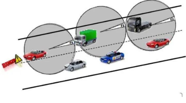
In the rest of this paper, we consider a traffic stream present on a straight line. This special case of inter-vehicle communication corresponds, in the vehicular context, to a transmission along a straight one way road or highway using a very directional antenna (see Figure 1). θ refers here to the angle of transmission. In case of a directional antenna, this angle is very small. Observe that if all vehicles (including the source and the destination) are on a straight line, then the angle of transmission does not have any influence on the propagation of the message.
We assume that the vehicles are distributed on the line connecting the source and the destination according to a Poisson process of intensity λ. In other words, the distance between two consecutive vehicles follows an exponential
Fig. 1: Linear propagation scheme
distribution. The average distance between two vehicles is 1λ . This assumption is based on some traffic studies that have proved that the inter-vehicle spacing on a highway can be modeled by an exponential distribution [2].
In what follows, we present an analytical model for the probability of success and also the average number of hops. Simulations will also be conducted to validate the models.
IV. PROBABILITY OF SUCCESS
A. Analytical model
As mentioned above, we assume that the vehicle position is confined to one dimension (single line). The vehicles spatial positions are modeled as a Poisson process of intensity λ. We consider also a fixed transmission power for all nodes. Thus, all vehicles have the same fixed transmission range denoted as r.
Initially, a sender vehicle (1) generates an alert message that has to be forwarded by other vehicles (see Figure 2). We assume also that each node only forwards the message once since it can recognize later copies of the original broadcast. We denote by d the distance between the sender S and the destination D.
Fig. 2: One dimension Broadcasting scheme
We will compute the probability of success though recursive formulas.
To evaluate this probability, we can assume that after the emission of the first message, by the source S, the farthest node from S will be the next relay. In other words, the message will reach the destination if two conditions are satisfied: first
there are other nodes within a distance r from S, and second the message sent by the farthest node from S (among those that are within a distance r) should reach the destination. Consequently, one may think that the whole probability of success is obtained by considering all possible positions x of the farthest node and then multiplying by the probability of success from the position x.
In other words, one may think that this probability is given by S(d) =R0re−λ(r−x)S(d − x) dx where e−λ(r−x) represents
the probability that there are no nodes in the interval [x,r], λ dx represents the probability to have a node around the position x while S(d − x) is the probability to reach the destination from the farthest node (the distance between the farthest node and the destination is d− x). The formula above is unfortunately not correct because there is some dependency between the probabilistic events ”the farthest node has the position x” and ”the message sent by the farthest node reaches the destination”. Knowing that there are no nodes in the interval [x,r] has definitely some correlation with the success probability of any transmission initiated from this node.
One way to overcome this difficulty is to assume that the closest vehicle (instead of farthest) is relaying the message. As observed by [8], this assumption does not have any impact on the probability of success. Then the following recursive formula is valid:
S(d) = Z r
0
e−λxS(d − x) dx (1)
Formula (1) can be used to compute the success probability (or more precisely to approximate it). However, we will introduce another recursive formula to compute the success probability. The main reason for that is that what will be computed in this section, will be useful to compute the average number of hops in the next section.
Observe that assuming that the farthest node located in position x is transmitting the message within a distance r is in fact equivalent to assume that there is a node located in position r transmitting within a distance x.
Then, in order to compute the probability of success, we have to introduce the quantity S(d, a) representing the probability of success knowing that the first node (source) is transmitting within a range a, where 0 < a ≤ r, while all relays transmit within a distance r.
While we are only interested in computing S(d, r), we must compute S(d, a) for different values of d and a.
Figure 2 represents the situation described above. The first vehicle (S) will transmit the broadcast message with a range a, where 0 < a ≤ r, while the farthest vehicle transmits within a distance r.
The probability of success is now given by the following recursive formula for 0 < a ≤ r:
S(d, a) = Z a
0
λe−λ(a−x)S(d − a, r − a + x) dx (2) In this equation, λdx refers to the probability of having a node around x, while e−λ(a−x) represents the probability of absence of any vehicle within the interval [x,a]. As explained above, the emission of a message within a distance r by a
vehicle located in position x is equivalent to the emission of a message within a distance r−a+x by an ”imaginary” vehicle located in position a.
In order to exploit the recursive formula (2) to compute the numerical values of S(d, a), we will discretize the interval [0,
a]. More precisely, we assume that:
r = kb
d = lb (3)
a = ib
Where b is a small distance called a step and i, l and k are integers. b can be seen as a precision factor in order to determine the probability of success. In fact, the smaller it is, more precise the probability will be.
Hereafter, we give some obvious upper and lower bounds of the probability of success.
By replacing a and x in the Eq.2, we obtain the probability of success transmission as:
S(lb, ib) = i−1 X j=0 Z (j+1)b jb
λe−λ(ib−x)S((l −i)b, (k −i)b+x) dx (4) The upper bound of the probability is obtained using the fact that S(d, a) increases when a increases.
Let us use S(lb, ib) (resp. S(lb, ib)) to denote the upper bound (resp. lower bound) of S(lb, ib).
Thus: S(lb, ib) =
i−1
X
j=0
λe−λibS((l−i)b, (k−i+j+1)b)
Z (j+1)b jb
eλxdx (5) corresponds to the upper bound.
Moreover, by calculating the integral in the Eq.5, we get: S(lb, ib) = i−1 X j=0 e−λb(i−j)(eλb− 1)S((l − i)b, (k − i + j + 1)b) (6) Using the same approach, we get the following lower bound for the probability of success.
S(lb, ib) =
i−1
X
j=0
e−λb(i−j)(eλb−1)S((l −i)b, (k −i+j)b) (7)
B. Model Validation
In this section, we evaluate the analytical model through numerous use cases. We also compare analytical results to simulation. Our goal is to verify the precision of the bounds given by Eq.6 and Eq.7.
As mentioned before, vehicles positions are generated ac-cording to a Poisson process. A sender station broadcasts an alert message that is received by its neighbor stations located on the straight line. Obviously, termination occurs when the distance between two adjacent relay nodes exceeds
r. In terms of simulation, we only have to iteratively generate the distances between consecutive vehicles according to an exponential distribution and continue doing that until either the destination is reached or the distance between two consecutive
nodes exceeds r. In the second case, we consider that there is a failure. By repeating these simulations many times, the ratio of simulations for which the message reached the destination provides an estimation of the probability of success.
Four levels of vehicle density are taken into account: λ= 0, 01; λ = 0, 02; λ = 0, 04; λ = 0, 05.
The probability of success (upper and lower bounds) is eval-uated against the results given by simulation. We will always assume that r= 200 m.
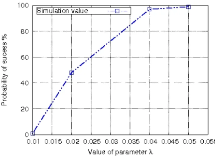
Fig. 3: Simulated values of probability of success Each simulation is repeated 10000 times. Figure 3 shows the average values of the probability of success obtained by simulation with d= 2000 m and r = 200 m. One can see that with λ = 0, 04, the probability of success is almost equal to 1. Notice that the average distance between two consecutive values is here given by 1λ = 25. In order to have a clear overview of the precision of our analytical model (with the precision step b= 5), we define the precision rate as follows: precisionrate= (1 − uppersimulationbound−lowerbound
value )100.
Our analytical model shows good performance in all cases (see Figure 4). Indeed, in the worse case, the precision of the model does not fall below 70% (λ= 0.01) and increases very quickly when λ increases.
For instance, for λ= 0, 02 and d = 2000 m, the analytical model gives: upper bound= 48.54% and lower bound= 47.80 %, while the simulated value of the probability of success is 48,51%.
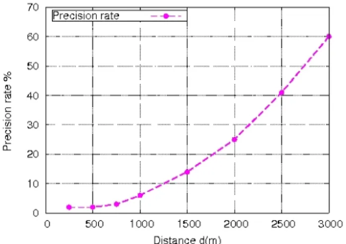
To measure the effect of the distance d on the broadcast operation, we ran the simulations for different distances shown by figure 5. Here b is equal to 5 and λ is equal to 0.02. Figure 5 shows again that the lower and upper bounds are very close to the simulated values.
We can also see that the probability of success decreases very quickly when d increases. For example, increasing the distance from1000 m to 4000 m reduces the probability from 70% to 20%.
In addition, if we plot the curve of the logarithm of the probability of success when d is varying from 1000 m to 8000 m, we can see that the curve is almost linear (see Figure 6).
Fig. 4: Precision of the probability model varying the density of vehicles
Fig. 5: Effect of distance on the broadcasting operation
This result may be justified as follows. If the distance d is large (compared to r), then one can expect S(2d, r) to be approximately equal to S2(d, r). Reaching a destination lo-cated at a distance2d is approximately equivalent to reaching a first destination located at a distance d and then restarting the transmission from this first destination and reaching a second destination located at a distance d from it.
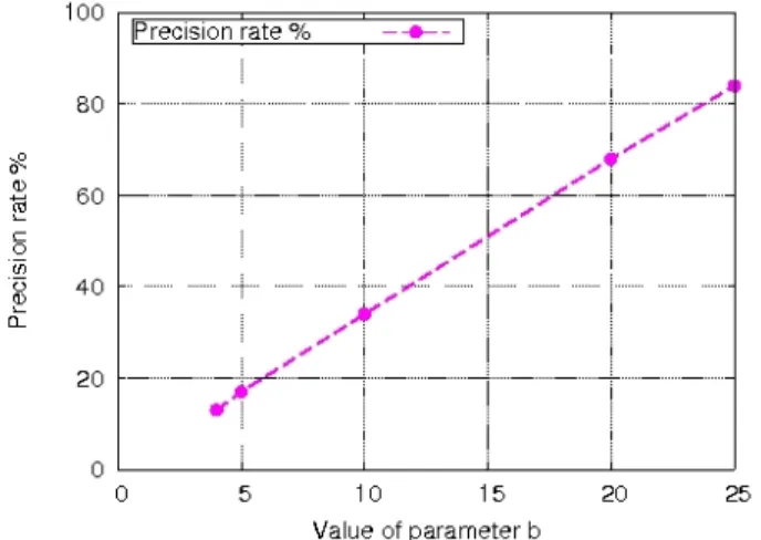
To better evaluate the influence of the parameter b on the precision of the lower and upper bounds more experiments are conducted. Figure 7 and 8 show the obtained results when λ= 0.02 and d = 4000 m.
Fig. 7: Effect of b variations on the probability of success
Fig. 8: Precision of the probability model when varying the parameter b
One can see that the difference between the lower and the upper bound increases when b increases. The precision rate shown on Figure 8 seems to vary linearly with b. As it can be seen from Figure 7 and the precision results, the smaller b is, the more accurate our bounds will be.
V. AVERAGENUMBER OF HOPS
To have a better understanding of the connectivity in VANETs, we investigate the average number of hops in the
shortest path linking the source to the destination (if there is any).
We will focus on the case when the message reaches the destination. An analytical model based on a recursive formula will be presented for the average number of hops.
A. Analytical Model
We still use the same notation as in the previous section. Let h(d, a) denote the average number of hops needed to propagate the message to a destination located at a distance d assuming that: the message reached the destination, the source is emitting within a range a, where0 < a ≤ r, while all relays transmit within a distance r. While we are mainly interested in computing h(d, r), we need to compute h(d, a) for different values of d and a.
Before presenting the recursive formula, we provide here some simple bounds related to h(d, r).
Proposition 1. ⌈d
r⌉ ≤ h(d, r) ≤ 1 + ⌈ 2d
r ⌉ (8)
Proof. The first inequality is obvious and well known. It is valid because the distance between two consecutive relays is less than r. The second inequality seems to be new. It can be proved very easily by observing that the distance between the relay number j (the jth vehicle forwarding the message) and the relay number j+ 2 is strictly larger than r. Adding up all inequalities for each j and rounding up leads to the wanted inequality.
Formula (8) clearly implies that the average number of hops is almost proportional to the distance. However, we should not forget that we are here making the assumption that the destination is reached.
Proposition 2. h(d, a) can be computed through the following recursive formula: h(d, a) = ( 1, if d ≤ a 1 + Rib 0 λe −λ(a−x)h (d−a,r−a+x)S(d−a,r−a+x) S(d,a) ,if d > a (9) Proof. Let h(d, a, j) denote the probability to reach the destination in j hops. if d≤ a we obviously have h(d, a) = 1 since the message sent by the source will reach the destination in one hop.
In the other case, the expected probability is given by: h(d, a, j) =
Z a 0
λe−λ(a−x)h(d − a, r − a + x, j − 1) dx (10) In this equation, λ dx refers to the probability of having a node around x, while e−λ(a−x) represents the probability of absence of any vehicle within the interval [x,a]. As explained before, the emission of a message within a distance r by a vehicle located in position x is equivalent to the emission of a message within a distance r−a+x by an ”imaginary” vehicle located in position a. The first message reaches the destination in j hops if and only if the message sent by this imaginary vehicle reaches the destination in(j − 1) hops.
Using Bayes’s rule, the average number of hops condition-ally to the success of the transmission is given by:
h(d, a) = ∞ P j=1 jh(d, a, j) S(d, a) (11)
where S(d, a) is still the probability of a successful transmis-sion from the source to the destination.
Replacing h(d, a, j) by its expression, Eq.11 becomes:
h(d, a) = ∞ P j=1 jR0aλe−λ(a−x)h(d − a, r − a + x, j − 1) dx S(d, a) (12) h(d, a) = Ra 0 λe−λ(a−x) ∞ P j=1 jh(d − a, r − a + x, j − 1) dx S(d, a) (13) Eq.13 can be rewritten as follows :
h(d, a) = Ra 0 λe −λ(a−x) ∞ P j=0 jh(d−a,r−a+x,j) dx S(d,a) + Ra 0 λe −λ(a−x)P∞ j=0 h(d−a,r−a+x,j) dx S(d,a) (14)
Using Eq.11 and Eq.2, Eq.14 becomes : h(d, a) = Ra 0λe −λ(a−x)h (d−a,r−a+x)S(d−a,r−a+x) dx S(d,a) + Ra 0λe −λ(a−x)S (d−a,r−a+x) dx S(d,a) = S(d,a)+ Ra 0λe −λ(a−x)h (d−a,r−a+x)S(d−a,r−a+x) dx S(d,a) = 1 + Ra 0 λe −λ(a−x)h(d−a,r−a+x)S(d−a,r−a+x) dx S(d,a) (15) This ends the proof of the proposition.
Observe that the recursive formula (9) includes the success probabilities S(d, a). That is why the success probabilities were calculated in the previous section.
Let us make the same assumptions given by Eq.3. Then, we get the following:
h(lb, ib) = 1+ i−1P j=0 R(j+1)b jb λe −λ(ib−x)h((l−i)b,(k−i)b+x)S((l−i)b,(k−i)b+x) dx S(lb,ib) (16) Using the upper and lower bounds of the probability of success computed before (S(lb, ib) and S(lb, ib)), upper and lower bound for h(lb, ib) can also be computed by dynamic programming.
Let us use hup(lb, ib) (resp. hlow(lb, ib)) to denote the upper
bound (resp. lower bound) of h(lb, ib).
Using the same approach than before (to bound the success
probability), we get the following bounds: hup(lb, ib) = 1+ i−1P j=0 e−λb(i−j) (eλb−1)hup((l−i)b,(k−i+j)b)S((l−i)b,(k−i+j+1)b) S(lb,ib) (17) hlow(lb, ib) = 1+ i−1P j=0 e−λb(i−j) (eλb−1)hlow((l−i)b,(k−i+j+1)b)S((l−i)b,(k−i+j)b) S(lb,ib) (18) We see again that after computing the upper and the lower bounds for the probability of success, it is possible to compute upper and lower bounds for h(lb, ib) by dynamic programming.
B. Simulation Results
Simulations are conducted as before. The distances between consecutive vehicles are generated according to an exponential distribution. Then, if the message reaches the destination, we just compute the length of the shortest path between the source and the destination.
The transmission range r is always equal to 200 m. In Figure 9, several simulations are performed with different vehicle densities λ. The distance d between the source and the destination is here equal to2000 m while we took b = 2. Lower bounds, upper bounds and simulated values are reported on Figure 9.
Fig. 9: The average number of hops: Simulation vs. analytical results varying λ
One can see that the lower and upper bound become very close to the simulated value when the density increases. Also observe that the average number of hops shown on Figure 9 becomes constant when λ increases. In fact, the average number of hops is almost equal to⌈d
r⌉ for high densities.
Moreover, several simulations are conducted with different values of d to evaluate the behavior of the upper and lower bounds (here b = 2 and λ = 0.02). Results are reported in Figure 11.
Fig. 10: Precision of the average number of hops model varying the density of vehicles λ
Fig. 11: The average number of hops: Simulation vs. analytical results varying d
The upper and the lower bounds seem to be very precise when the ratio dr is small. When the distance increases, since the bounds are computed by dynamic programming, there is an accumulation of errors leading to less and less precise bounds. This is confirmed by Figure 12 where the precision rate is reported with different values of d.
In order to study the effect of the parameter b on the precision of our model, we ran several simulations with different values of b.
Figure 13 reveals the performance of our analytical model when b is varying from 1 to 4 and for distance d= 2000 m. This is also shown on Figure 14 where the precision rate is reported.
One can deduce clearly that b has a great effect on the precision of our model.
In order to evaluate the effect of the distance of propagation
d, we make the same simulation with d equal to1000 m. Obtained results confirm that the model performs in a much more precise manner for distances smaller than the previous case (see Figure 15). This is due to the error accumulation
Fig. 12: Precision of the average number of hops model varying the distance d
Fig. 13: Effect of b variation in the average number of hop model
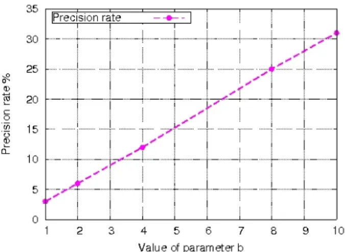
Fig. 14: Precision of the average number of hops model varying the parameter b (d= 2000 m)
Fig. 15: Precision of the average number of hops model varying the parameter b (d= 1000 m)
phenomenon. For example, for a distance d equal to 1000 m (resp.2000 m) and b equal to 4, the precision rate is equal to 12.2% (resp.52%). From a practical point of view, a distance of 2000 meters is a good upper limit for such category of emergency messages. Indeed, for safety applications [9] a distance of 1000 meters is the typical distance of a broadcast message to reach all the vehicles concerned by the alert.
VI. CONCLUSION
Analytical models are proposed to compute the end-to-end probability of success and the average number of hops in case of a successful linear transmission in a vehicular context. Several simulations have been performed to evaluate the precision of these models.
Mathematical expressions match very well the simulation results. As a future work, we are interested on information relay in the planar case. We also think that the case where vehicles are located on some successive straight lines can be modeled similarly to the linear case.
REFERENCES
[1] IEEE Computer society, IEEE standard for information technology,
telecommunications and information exchange between systems, local and metropolitan area networks - specific requirements - part 11: Wireless lan medium access control (MAC) and physical layer (PHY) specifications. IEEE Std 802.11-2007 (Revision of IEEE Std 802.11-1999).pages 1-1184, June 2007.
[2] N. Wisitpongphan, F. Bai, P. Mudalige, V. K. Sadekar, and O. K. Tonguz,
Routing in Sparse Vehicular Ad Hoc Wireless Networks, IEEE Journal on Selected Areas in Communications, vol. 25, no. 8, pp. 1538-1556, Oct. 2007.
[3] S.-I. Sou, and O. K. Tonguz, Enhancing VANET connectivity through
Roadside Units on Highways, IEEE Transactions on Vehicular Technol-ogy, vol. 60, no. 8, pp. 3586-3602, Oct. 2011.
[4] X. Wang, Modeling the process of information relay through intervehicle
communication, Transportation Research Part B: Methodological, Vol. 41, Issue 6, pp. 684700, July 2007. vol. 41, no. 6, pp. 684-700, Jul. 2007. [5] H.Takagi and L.Kleinrock, Optimal Transmission Ranges for Randomly
Distributed Packet Radio Terminals, IEEE Transaction on communication, vol. COM-32, no. 3, pp. 246-257, March 1984.
[6] W. Jin and W. W. Recker, Instantaneous information propagation in
a traffic stream through inter-vehicle communication, Transportation Research Part B: Methodological, vol. 40, no. 3, pp. 230-250, Mar. 2006.
[7] Y.-C. Cheng and T. G. Robertazzi, Critical connectivity phenomena in
multihop radio models, IEEE Transactions on Communications, vol. 37, no. 7, pp. 770-777, Jul. 1989.
[8] X.Wang, T. M. Adams, W.-L. Jin, and Q. Meng, The process of
infor-mation propagation in a traffic stream with a general vehicle headway: a revisit, Transportation Research Part C, pp. 367-375, 2010.
[9] C2C Consortium, CAR 2 CAR Communication Consortium Manifesto, August 2007.