Seeing it all: Convolutional network layers map the function of the human visual system

HAL Id: hal-01389809

https://hal.inria.fr/hal-01389809

HAL is a multi-disciplinary open access archive for the deposit and dissemination of sci-entific research documents, whether they are pub-lished or not. The documents may come from teaching and research institutions in France or abroad, or from public or private research centers.

L’archive ouverte pluridisciplinaire HAL, est destinée au dépôt et à la diffusion de documents scientifiques de niveau recherche, publiés ou non, émanant des établissements d’enseignement et de recherche français ou étrangers, des laboratoires publics ou privés.

function of the human visual system

Michael Eickenberg, Alexandre Gramfort, Gaël Varoquaux, Bertrand Thirion

To cite this version:

Michael Eickenberg, Alexandre Gramfort, Gaël Varoquaux, Bertrand Thirion. Seeing it all: Convo-lutional network layers map the function of the human visual system. NeuroImage, Elsevier, 2016, �10.1016/j.neuroimage.2016.10.001�. �hal-01389809�

Seeing it all: Convolutional network layers map the

function of the human visual system

Michael Eickenberg1,3∗_{, Alexandre Gramfort}2,3_{, Ga¨el Varoquaux}1,3_{, Bertrand Thirion}1,3

1 Inria Parietal Team, Inria Saclay, France

2 CNRS LTCI, T´el´ecom ParisTech, Universit´e Paris-Saclay

3 Neurospin, I2BM, DSV, CEA Saclay ∗ E-mail: michael.eickenberg@inria.fr

Abstract Convolutional networks used for computer vision represent candidate models for the computations performed in mammalian visual systems. We use them as a detailed model of human brain activity during the viewing of natural images by constructing predictive models based on their different layers and BOLD fMRI activations. Analyzing the predictive performance across layers yields characteristic fingerprints for each visual brain region: early visual areas are better described by lower level convolutional net layers and later visual areas by higher level net layers, exhibiting a progression across ventral and dorsal streams. Our predictive model generalizes beyond brain responses to natural images. We illustrate this on two experiments, namely retinotopy and face-place oppositions, by synthesizing brain activity and performing classical brain mapping upon it. The synthesis recovers the activations observed in the corresponding fMRI studies, showing that this deep encoding model captures representations of brain function that are universal across experimental paradigms.

1

Introduction

Human and primate visual systems are highly performant in recognizing objects and scenes, providing the basis of an excellent understanding of the ambient 3D world. The visual cortex is hierarchically organized, which means that many functional modules have feedforward and feedback connections compatible with a global ordering from lower levels to higher levels [1]. The concept of visual “pathways” or “streams” [2, 3] is an established pattern which identifies principal directions of information flow for specific tasks, namely object representation in the “ventral stream” (from occipital cortex into temporal cortex) and localization and spatial computations in the “dorsal stream” (from occipital cortex into parietal cortex). They share much processing in the occipital early visual areas and less oustide of them. The ventral visual stream encompasses visual areas V1, V2, V3, V4 and several inferotemporal (IT) regions. Pure feedforward pathways from V1 to IT (via other areas) exist, and probably account for rapid object recognition [4, 5].

Many parts of the human and primate visual cortices exhibit retinotopic organization in so-called visual field maps: The image presented to the retina is kept topographically intact in the next processing steps on the cortical surface [6]. This results in a one-to-one correspondence between a point on the retina and the “centers of processing” for that point in the visual field maps, such that neighboring points on the retina are processed nearby in the visual field maps as well.

The seminal work of [7] showed that cat and other mammal V1 neurons selectively respond to edges with a certain location and orientation in the visual field.

This discovery inspired a long line of research investigating the nature of the computa-tions performed in other visual regions and how they are implemented. As an example, certain monkey V2 neurons were found to react to combinations of orientations, such as

corners [8]. Recently, it has been put forward that V2 may be an efficient encoder of expected natural image statistics arising from interactions of first-order edges [9]. V4 is reported to respond to more complex geometric shapes, color, and a large number of other stimulus characteristics. Recently it has been posited that V4 performs mid-level feature extraction towards the goal of bottom-up and top-down figure-ground segmentation [10]. Further down the ventral pathway, neurons in the IT cortex have been shown to be selective to parts of objects, objects and faces [11, 12]. Taken together, these findings indicate an increasing trend in abstractness of the representations formed along the ventral stream.

FMRI has been used very successfully to identify and delineate the aforementioned visual field maps as well as brain regions that seem to specialize to certain tasks in the sense that their responses are particularly strong for specific types of stimuli. This type of result has typically been derived using statistical contrast maps opposing various visual stimuli. The contributions [13–15], for instance, use this technique to localize specialized regions: areas for faces, body parts, places. Finer models, known as “encoding” models or forward modeling techniques [16], have been used to study the brain response to stimuli in greater detail [17–19]. This setting usually relies on richer models, going beyond binary contrasts, towards a more open description of the link between stimulus and activation. The validity of the corresponding stimulus representation is then established by testing how well it predicts brain activity, often with a linear model, by using cross-validation on held-out data.

For example, in [17], almost 2000 naturalistic images were used as stimuli and the BOLD signal responses were then fit using a predictive model based on Gabor filterbank responses of the images shown. Primary visual cortex was very well modeled, but also extrastriate areas such as visual area V4 were well explained by the Gabor filter model.

convolu-tional networks for object recognition to model human brain activity. We create encoding models [16] from the processing layers of the convolutional network OverFeat [20], which each represent feature maps at different levels of complexity. We train a linear predictive model of brain activity for each of the layers on the datasets of [17] and [21] and compare their ability to describe brain activity for every voxel by evaluating the predictive score on held-out data.

The scores of the different layers outline continuous progression profiles that are distinct in each visual area. We demonstrate that the model captures the cognitive architecture of the visual system by investigating its generalization capacity to visual-neuroscience paradigms beyond natural-image viewing. To do so we use stimuli unseen by our model, of which some come from totally different experiments and follow vastly different pixel statistics. Our predictive model, which can be seen as data-driven forward model to generate fMRI activations, is used to synthesize putative brain activation maps corresponding to these novel stimuli. This methodology enables our model to reproduce classical experiments in the extensive literature of paradigm-driven fMRI research. We consider two of these experiments: retinotopic mapping, i.e. the capturing of spatial information to sufficient accuracy for the generation of visual field maps, and a faces/places contrast to capture high-level information.

Previous work has used convolutional networks with fMRI data [23, 24]. However it focused on specific experiments. Showing that results generalize across datasets and paradigms brings an important novel step to the use of convolutional networks for the study of human vision. First, we show the validity of the approach on a new dataset with videos rather than still images. Second, we synthesize plausible brain activity to new images from completely different experiments that rely on hand-crafted, well controlled stimuli. These results demonstrate that convolutional networks capture universal representations

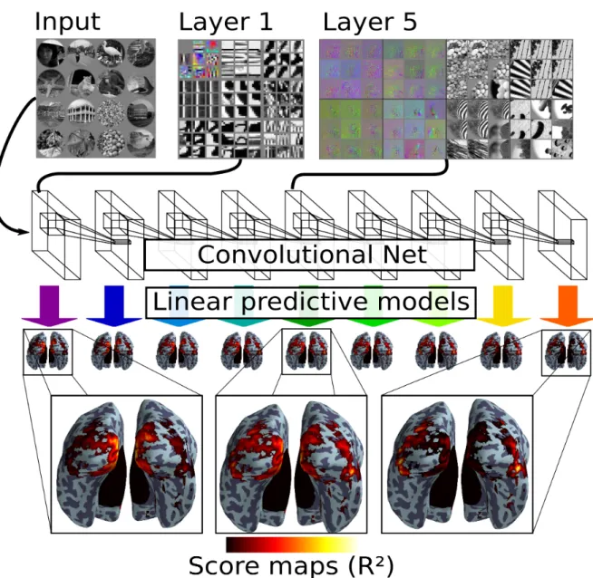
Figure 1: The experimental setup. Top left: 16 Examples of stimulus images (similar in content to the original stimuli presented to the subjects, and identical in masking) which are input to the convolutional network. Top middle: Selected features of first layer (top left of panel) and image patches activating these features (other eight panels). Top right: Image space gradients of selected feature maps from layer 5 (left panel) and example patches driving these feature maps. The gradients show which change in the image would lead to a stronger activation of the feature map (see [22]). Middle: Depicts convolutional net layers. Every layer is evaluated for its predictive capacity of all the voxels. For each layer, the corresponding predictive model is depicted by an arrow pointing downward from the convolutional net. It yields a score for each voxel, giving rise to a map of the brain, depicted below the arrow. Bottom: The close-up views are intended to highlight different areas that are well modeled: The first layer models best medial occipital regions close to the Calcarine fissure, the last layer explains more variance in lateral and inferior occipital regions. The middle layer shows an intermediate score map between the two extremes.

of the stimuli that linearly map to and separate cognitive processes, such that this link generalizes to unseen experimental paradigms.

2

Biological relevance of multi-layer vision models

The Gabor filter pyramid employed in the original work of [17] can be seen as an instance of a biologically inspired computer vision model. Indeed, all of modern computer vision, in its roots, has been inspired by biological vision. The basic filter extraction techniques at the beginning of the most successful computer vision pipelines are based on local image gradients or laplacians [25, 26], which are operations that have been found in V1 as edge detection and in the LGN as center-surround features. The HMAX model was constructed to incorporate the idea of hierarchies of layers [27]. HMAX models are layered architectures that typically begin with edge detection using oriented filters, followed by a spatial and across-channel max-pooling. Subsequent layers implement other forms of localized (convolutional) processing, such as linear template matching. Using a supervised classifier at the end of this processing, it reached near state-of-the-art object recognition capacities in [28].

The natural question to ask in the context of predictive modeling of BOLD fMRI in visual areas is “What comes after the Gabor filter pyramid?”. The scattering transform model [29, 30] provided only one supplementary layer of which one cannot state much more than the existence of brain voxels which it models well [31]. The scattering transform is a cascade of complex wavelets and complex moduli, which has good mathematical stability properties and yields rich representations. The layers C1 and C2 of HMAX as used in [28] were obtained using random templates taken from the preceding pooling layer activation. They were not geared optimally towards object recognition. This made the difference

between layers difficult to evaluate (see e.g. [32]). Although quite similar in architecture, deep artificial neural networks are of much greater interest here. Indeed, they optimize intermediate layers towards increasing overall performance in object detection, which is known to be performed also in IT cortex in humans and primates (see [33], [32]).

Artificial neural networks for computer vision attain state-of-the-art results with optimized feature hierarchies in a layered architecture composed of stacked layers with units that compute a linear transformation of the activations of previous layers followed by a simple pointwise nonlinearity. For instance, the first linear transformations are typically similar to Gabor filters and the corresponding non-linearities perform edge detection. Recent breakthroughs in the field of artificial neural networks have led to a series of unprecedented improvements in a variety of tasks, all achieved with the same family of architectures. Notably in domains previously considered to be the strongholds of human superiority over machines, such as object and speech recognition, these algorithms have gained ground, and, under certain metrics, have surpassed human performance [34].

Bridging to neuroscience, [33] and [35], using electrophysiological data, have shown that IT neuron activity is predictive of object category in a similar way as the penultimate layer of a deep convolutional network which was not trained on the stimuli. Even more striking: a deep convolutional network can predict the activity of IT neurons much better than either lower-level computer vision models or object category predictors. Furthermore, deep convolutional networks trained on object categories and linked to neural activity with simple linear models predict this neural activity as well as the same network trained directly on neural data, suggesting that the encoding of object categories in the network is a good proxy for the representation of neural activity. These two works inspired us to investigate the link between computer-vision convolutional networks and brain activity with fMRI in order to obtain a global view of the system. Indeed, fMRI is much more

noisy and indirect than electrophysiological data, but it brings a wide coverage of the visual system.

Inspection of the first layer of a convolutional net reveals that it is composed of filters strongly resembling Gabor filters, as well as color boundaries, and color blob filters (shown at the top of Fig. 1). These features are similar in nature V1 receptive fields. To understand the other end of the hierarchy, close to the output of a convolutional network, we apply the successive transformations of such a network to a natural image representing object categories. This most often yields a correct object identification (classification rates have risen from around 80% to around 96% over the 1000 object categories of imagenet in the last 3 years [36, 37]). Since this classification is a linear transformation of the penultimate layer representation space from which one can also predict IT neural activity linearly, there must be a correspondence in representation. Indeed, there exist high-level visual areas tuned to specific object categories: body parts, faces, places.

We have thus established that there are similarities between the computations of convolutional networks and cognitive vision at the beginning and at the end of the ventral stream object-recognition process. Evaluating its intermediate layers with respect to how well they explain activity in visual areas of the brain is a stepping stone towards a bigger picture of the correspondence.

3

Methods

3.1

Datasets

We consider two different datasets of BOLD fMRI responses to visual stimulation of very different nature: still images and videos. The still images dataset [38] originates from [17] and [18]. 1750 gray scale natural images in a circular frame of visual angle 20 degrees were

presented at an interstimulus interval of 4s for the duration of 1s in three flashes “ON-OFF-ON-OFF-ON”, each “ON” and “OFF” phase of 0.2s duration. The content of the photos included animals, buildings, food, humans, indoor scenes, manmade objects, outdoor scenes, and textures, taken from the Corel Stock Photo Libraries from Corel Corporation, Ontario, Canada, the Berkeley Segmentation Dataset, and the authors personal collections. Each image was shown twice in total, in the same scanner run, to subjects fixating a central cross. Every eighth stimulus presentation were uniform gray empty events. 25 scanner runs divided into 5 scanner sessions we acquired 1. 120 validation images were presented during 10 scanner runs divided into the same 5 scanner sessions. Each validation image was presented 13 times overall. BOLD signal acquisition was performed using a surface coil in 18 coronal slices of matrix size 64x64, slice thickness 2.5mm, in-slice sampling 2mm x 2mm, repetition time TR=1s. Reconstruction was performed using ReconTools2_.

A phase correction was applied to reduce Nyquist ghosting and image distortion. Slice timing correction was done via sinc interpolation. After motion correction and manual realignment of scanner runs, the multiple responses to each image were averaged into one activation map using a GLM model with an individual hemodynamic response function per voxel, estimated using alternate optimization and a low-frequency Fourier basis for the HRF function. We work with the obtained activation maps and the stimuli. ROI boundaries were obtained by standard retinotopic mapping.

Data from two healthy subjects with normal or corrected-to-normal vision are available in [38].

The video stimulus was first presented in [19] and used also in [21]. It consists of movie trailers and wildlife documentaries cut into blocks of 5-15 seconds and randomly shuffled.

1_{A scanner session is the full amount of time spent in the scanner from entrance to exit and usually}

lasts around 90 minutes. A scanner run is a continuous sequence of measurements. Several runs can take place during a session, separated by short breaks.

A train set of two hours duration and no repetition was separated from a test set in which around 10 minutes of unique stimulus were cut into blocks of around 3 minutes and repeated in random order 10 times each. Subjects fixated a central cross while passively viewing these stimuli. 30 axial slices of 4mm thickness were acquired, covering the full brain. In-slice sampling was 2mm x 2mm. The acquired data were motion corrected and manually realigned. The ten runs of the validation set were averaged to reduce noise. This dataset comprises one subject.

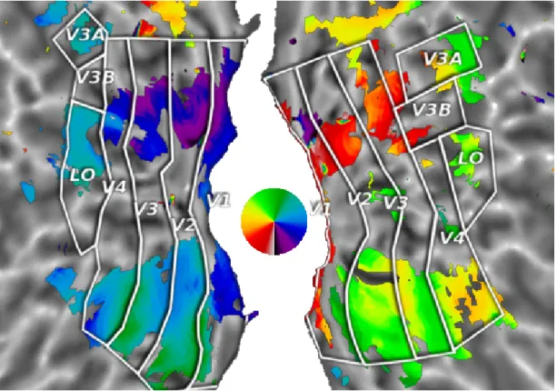
Both datasets provide functionally localized regions of interest. Visual areas V1, V2, V3, V4, V3A, V3B and LOC were determined using phase-coded retinotopic mapping. All surface projections were computed and flatmap diagrams were created using the pycortex software [39]. ROI boundaries were outlined according to localized maps, provided as volume maps in the dataset of [17] and as outlines for the data from [21]. Volume ROIs were projected to the surface using a nearest neighbor projection and outlines drawn along the borders of the projections.

3.2

The encoding pipeline

We chose the “large” version of the deep convolutional net “OverFeat” [20] to run our analyses. It features six convolutional layers and three fully connected ones. Details can be found in [20]. Here, we are interested in convolutional networks not to classify images, but as a means to transform them into successive intermediate representations: from Gabor-like features to abstract shapes (see Fig. 1). Using the sklearn-theano3 _{software, the network}

was applied to all stimulus images and the outputs of all neural network layers kept. Since the intermediate representations are rather large (e.g. ∼ 106 _{features on the first layer),}

each channel of each layer was spatially smoothed and subsampled to achieve a number of

features of around 25000 per layer. This was achieved by determining the smallest integer spatial subsampling necessary to obtain 25000 features or less: for instance, the first layer having 96 × 113 × 113 = 1225824 features, a spatial subsampling of factor 8 per axis is necessary to bring the number of features down to 1225824/(8×8) ≈ 19154. The smoothing parameter for the Gaussian is set to 0.35 × d, where d is the downsampling factor (here 8). For the video data, sampled at 15 Hz at an acquisition TR of 2 s, temporal downsampling was additionally performed by calculating the temporal mean across 30 frames at a time. A compressive non-linearity, log(1 + x) was applied pointwise, similarly to the procedure described in [16]. Using only the stimuli from the training set, `2-penalized linear regression

(ridge regression) was used to fit a forward model for the outputs of each layer for each brain voxel. The choice of Ridge regression is due to practical considerations such as computation speed and simplicity. Better model selection could be attempted with a penalty enforcing exact zeros, such as the `1-norm or group-structured norms grouping features located

in one place. However, for the given data shape this is prohibitive in computational resources. Contrary to [33], we employ a linear kernel instead of a Gaussian one. In addition to the isotropic `2-penalty, a Gaussian kernel has a hyperparameter controling the

kernel width, providing a continuous ensemble of models ranging from nearest-neighbor-to linear-projection-based predictions. [33] studied the full hyperparameter path while predicting from the last layer. Nearest-neighbor type decisions, unlike linear decisions, indicate a complicated decision boundary and thus do not reveal as simple representation of brain activity. Here we work only with linear decision boundaries in order to be able to compare the complexities of the convolutional network layers on as equal footing as possible.

For the video data, temporally lagged copies of the outputs at t-4, t-6 and t-8 seconds were used in order to take into account the hemodynamic lag.

We proceed by evaluating how well the activity of each brain voxel can be modeled by each of the OverFeat layers separately. The fitted model was evaluated in a K-Fold cross-validation scheme with bagging. The training data were themselves divided into train/test splits (in accordance with scanner sessions: “leave one session out”, K=5 for images, K=3 for videos) and a model trained on an inner train split was evaluated on the corresponding test split to select an optimal penalty. Model scores were obtained using predictive r2 _{score for the dataset of [17]. This means that for a voxel v the}

activation yv_test for the test set images was compared to the prediction by our model yv_pred as follows: r2_v = 1 − ky

v

test−ypredv k

2

kyv

test−mean(yvtest)k2, where mean(y

v

test) is the mean activation

of voxel v on the test set. Video predictions were evaluated using correlation score rv =

hyv

pred−mean(ypredv ),yvtest−mean(ytestv )i

kyv

pred−mean(yvpred)kkyvtest−mean(yvtest)k. The optimal models for each train/test split of the train data were averaged in order to gain stability of predictions. Mean scores over folds for the optimal penalty were kept as a quantitative measure of goodness of fit.

For further analysis we keep all voxels up to a false discovery rate (FDR) [40] of 0.01. In order to obtain a selection criterion we choose the maximal score over all layers as a statistic. This choice is necessary due to the fact that we cannot know a priori which layer will describe the voxel’s activity well. The null distribution of these maximum layer score values was obtained by a permutation test (100,000 permutations) on 14 different voxels distributed across the brain volume. Comparison of the histograms of the obtained distributions showed that they are essentially identical and can be used as a global null hypothesis for all brain voxels. The FDR was evaluated using the p-values for every voxel calculated from an empirical distribution obtained by concatenating all permutations over the 14 voxels.

A schematic4 of the encoding model is provided in Fig. 1. The lowest level layer is

4_{All artificial neural network layers are depicted as being convolutional, although the last three are what}

depicted on the left and the highest level layer on the right. The surface images below each layer show an r2 score map for the predictive model learnt on this layer. The scores are normalized per voxel such that the sum of scores across layers is 1. This accounts for differences in signal-to-noise ratio across brain regions and highlights the comparison of layers.

In the results section (4), we use these voxel-level prediction scores with a per-ROI analysis of the cross-layer profile of reponses and a more systematic mapping of layer preferences across all voxels that are well-explained by the model.

3.3

Synthesis of visual experiments

Using the predictive models learnt on each convolutional network layer, we build a simple summary model by averaging all layer model predictions for each voxel. We validate the predictive capacity of this averaged model by using it as a forward model able to synthesize brain activation maps: Using the ridge-regression coefficients, our model predicts full brain activation maps (“beta maps”) from new stimuli.

These activation maps can be understood using the standard-analysis framework for brain mapping, in which one evaluates a general linear model with relatively few condition regressors, e.g. contrasting the activation maps between two different experimental conditions.

We propose to revisit two classic fMRI vision experiments, retinotopy and the faces versus places contrast, by generating them with our forward model. Since these are known experiments, they can be compared and interpreted in context. At the same time, they test different levels of complexity of our model. Retinotopy is purely bound to receptive field location which captures global coarse-grain organization of the images, while the convolutions and [20] takes advantage of this to perform detection and localization.

distinction of faces necessitates higher-level features that are closer to semantic meaning. Note that retinotopic mapping was also used in the original study [17] to validate the forward model estimated using Gabor filters. In contrast to our setting, retinotopy was estimated by localizing receptive field maxima for each voxel instead of using the predictive model as a data synthesis pipeline.

3.3.1 Retinotopy

We created “natural retinotopy” stimuli (see [41]) by masking natural images with wedge-shaped masks. The wedges were 30◦ wide and placed at 15◦ steps, yielding 24 wedges in total. After creation of exact binary masks, they were slightly blurred with a Gaussian kernel of standard deviation amounting to 2% of the image width. We chose 25 random images from the validation set of [17] and masked each one with every wedge mask.

The thus obtained set of 600 retinotopy stimuli were fed through the encoding pipeline to obtain brain images for each one of them. These brain images were then used for a subsequent retinotopy analysis. The design matrix for this analysis contains the cosine and the sine of the wedge angle of each stimulus and a constant offset. The retinotopic angle is calculated from the arising beta maps by computing the arctangent of the beta map values for the sine and cosine regressors. Responsiveness of the model to retinotopy was quantified by the F-statistic of the analysis. In order to obtain an easily interpretable retinotopic map, the beta maps were smoothed with a Gaussian kernel of standard deviation 1 voxel before the angle was calculated. Display threshold is set at F > 1.

3.3.2 Synthesizing a “Faces versus Places” contrast

Discriminating faces from places involves-higher level feature extraction. While, with certain stimulus sets, the distinction can also be done based on low-level features such as

edge detectors, this is almost certainly untrue for the mechanism by which mammalian brains process faces due to the strong invariance and selectivity properties with respect to nontrivial transformations that they can undergo (see [42] for a discussion). In this sense, being able to replicate a “faces versus places” contrast with the proposed brain activity synthesis is a test for the ability to reproduce a higher-level mechanism.

We compute a ground-truth contrast against which we test our syntheses by selecting 45 close-up images of faces and 48 images of scenes (outdoor landscapes as well as exteriors and interiors of buildings from the dataset of [17]). Examples similar to the original stimulus and identical in masking are depicted in Fig. 6 (A). The 45 face images used were the only close-up images of human faces in the dataset. All other photos with faces were either taken at a distance, of several persons at once, or of human statues or animal faces. All images are unique in content. No slightly modified (e.g. shifted) copies of any image exists in the dataset. Using a standard GLM, we compute a contrast map for “face > place” and “place > face”, which are shown in Fig. 6 (C), thresholded at t = 3.0 in red tones and blue tones respectively.

Our first experiment is to synthesize brain activity using precisely the 93 images which produced the ground truth contrast. We trained our predictive model on the remaining 1657 training set images of [17] after removal of the 93 selected face and place stimuli. As stated above, these remaining images do not contain any images simply related to faces. After computing the synthesized activation images for the latter, we proceeded to analyze them using the same standard GLM procedure as above for the ground truth.

Due to the fact that the noise structure of the synthetic model is different, the threshold of the generated contrast must be chosen in a different manner. We use a precision-recall approach that can be described in the following way: Having fixed the threshold of the ground truth contrast at t = 3.0, we define the support of the map as all the voxels

that pass threshold. For a given threshold t on the synthesized map we define recall as the percentage of the support voxels from the ground truth contrast that are active in the thresholded synthesized map and precision as the percentage of active voxels in the thresholded synthesized map that are in the support of the ground truth map. We define the synthesized map threshold tR50 as the threshold guaranteeing a minimum of 50% recall

while maximizing precision.

Our second experiment tests the generalization capacity of our model in a more extreme situation: In order to make sure that our feedforward model is not working with particularities of the stimulus set other than the features relevant to faces and scenes, we also used our model to generate a faces-versus-places opposition using stimuli from [43]. These stimuli were originally used to show distributed and overlapping representations of different classes of objects in ventral visual areas. Among the stimuli are 48 pictures of faces and 48 pictures of houses. These stimuli are notably different in appearance from the ones used to train our model: they are centered and scaled, and tightly segmented on a light gray background, while the images used to train the model are natural images, with objects of varying size and position on a busy background (see figure 6(A) and (B)). We applied the same feedforward pipeline to synthesize activation maps from each of these images and the same GLM analysis and thresholding procedure as described in the preceding experiment.

4

Experimental results

All experimental results were obtained on volume data. For visualization purposes they were subsequently projected to surface maps. In the case of the images dataset, this projection is slightly distorted in areas distant from the occipital pole. Furthermore, the

field of view of the acquisition is restricted to the occipital lobe. On inspection of the three zoomed panels from Fig. 1 one observes that the score maps are different across layers. On the left, the model based on the first layer explains medial occipital regions well with respect to the others. It includes the calcarine sulcus, where V1 is situated, as well as its surroundings, which encompass ventral and dorsal V2 and V3. This contrasts to the score map on the right, which represents the highest level model. The aforementioned medial occipital regions are relatively less well explained, but lateral occipital, ventral occipital and dorsal occipital regions exhibit comparatively higher scores.

4.1

Quantifying layer preference

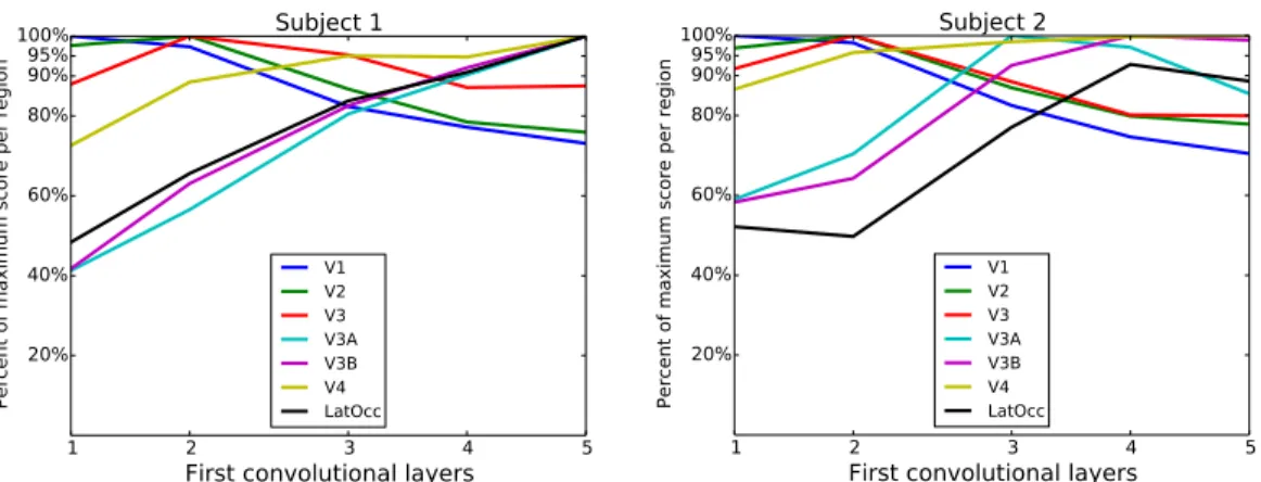
For each voxel, we call the set of scores associated with the prediction of its activity from each layer the score fingerprint of that voxel. Given the fact that layer outputs are correlated (across layers) and each voxel contains many neurons, we do not expect sharp peaks in the score fingerprint for a specific “best” layer. Rather we expect a progression of scores over layers indicating a global trend towards simple, intermediate or more high-level representations. Using the ROI definitions provided by the datasets, we can study the mean score fingerprints per region of interest. The average score fingerprint per ROI was obtained using the 25% best predicted voxels within the region. For each region of interest, the mean score fingerprint was normalized by its maximum value. The resulting normalized progressions are shown in Fig. 2.

We observe that for both subjects, the score fingerprint for V1 peaks at the first layer. It then decreases in relative accuracy as the layer index increases. For the mean fingerprint of V2, the peak lies on the second layer and the subsequent decrease is a little slower than that of the V1 fingerprint. This indicates that V2 is selective for a mix of higher-level features less present in V1. The V3 mean score fingerprint also peaks at

1 2 3 4 5

First convolutional layers

20% 40% 60% 80% 90% 95% 100% Percent of maximum sco re per region Subject 1 V1 V2 V3 V3A V3B V4 LatOcc 1 2 3 4 5

First convolutional layers

20% 40% 60% 80% 90% 95% 100% Percent of maximum sco re per region Subject 2 V1 V2 V3 V3A V3B V4 LatOcc

Figure 2: Normalized average score fingerprints over ROIs. Score progressions

for two subjects averaged over regions of interest provided by the dataset. For each ROI, the score progression was normalized by its maximally predictive layer score. For V1 we observe peak score in layer 1 and a downward trend towards higher level layers. The V2 fingerprint peaks in the second layer and then decreases slightly slower than the V1 fingerprint. V3 fingerprint also peaks in layer 2 but decreases more slowly than V1/V2 fingerprints. V4 fingerprint peaks much later than the ones of V1/V2/V3 but is not much worse described by lower level layers. Fingerprints of V3A/B and LOC show a strong increase across layers.

layer 2 and decreases less fast than the V2 fingerprint, indicating a selectivity mix of again slightly higher levels of representation than present in V2. The mean V4 fingerprint peaks significantly later than the first three, around layers 4 and 5. V4 is, however, well explained by the complete hierarchy of features: the score fingerprint is constantly above 70% of its maximum score. In contrast, the dorsal areas V3A and V3B are much less well modeled by lower level layers than by higher level layers. Similarly, the lateral occipital complex (LOC) shows a strong increase in relative score with increasing representation layer number.

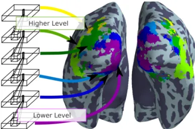
In Fig. 3 we show a winner-takes-all (“argmax”) map over spatially smoothed scores (σ = 1 voxel). It is obtained by smoothing each score map and then associating each voxel with the layer which best fitted its activity. This marker provides compelling outlines of the organization of the visual system: the map of which layer of the convolutional

Figure 3: Best model per voxel. Among the voxels which are modeled by at least one of the convolutional network layers, we show which network layer models which region best. This is achieved by smoothing the layer score maps (σ = 1 voxel) and assigning each voxel to the layer of maximal score. One observes that the area around the Calcarine sulcus, where V1 lies, is best fit using the first layer. Further one observes a progression in layer selectivity in ventral and dorsal directions, as well as very strong hemispheric symmetry.

network explains best brain activity segments the organization of the visual system well. One observes that medial occipital regions are mostly in correspondence with the first layer, that there is a progression in layers along the ventral and dorsal directions, which is symmetric, and that there is a global symmetry across hemispheres.

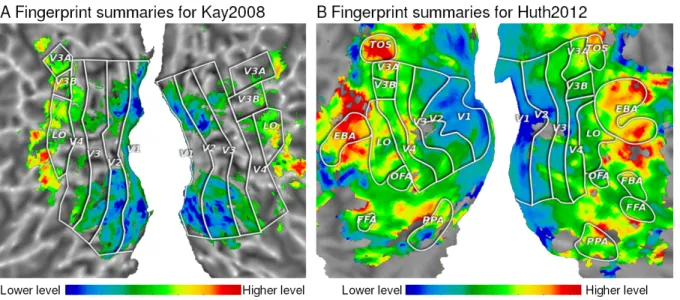
In order to better show the layer selectivity of each voxel as represented by its score fingerprint in a brain volume, we derived a summary statistic based on the following observation. As can be seen in Fig. 2, the average fingerprints of each region of interest have either an upward or a downward trend. It turns out that the first principal component of all score fingerprints over significantly well predicted voxels is a linear trend. Moreover, it explains over 80% of the variance of all fingerprints. The projection onto it can therefore be used as a summary of the voxel fingerprint. Here we use a fixed trend going from -1 at layer 1 to 1 at layer 9 in steps of 0.25. Projecting the score fingerprints onto this

Figure 4: Fingerprint summaries as brain map. We compute a summary statistic for voxel fingerprints by evaluating their inner product with an ascending linear trend from -1 to 1 in nine steps of 0.25. This yields low values for low layer preference and high values for late layer preference. Observe the preference for low-level models in earlier visual areas V1 and V2. With increasingly higher layer selectivity for V3, V4 and ulterior visual areas, a trend from low level to high level representation across the ventral and dorsal visual pathways becomes apparent.

ascending trend, which amounts to evaluating the global slope, yields a summary of the voxel fingerprint. It is shown for subject 1 in Fig. 4 on the left. We observe that V1 fingerprints project almost entirely to the low level range of models, indicated by blue hues. V2 shows more presence of green, indicating intermediate level models. This trend continues in V3. V4 shows a clear preference for mid-level models. Subsequent regions show a tendency towards even higher level representations.

This progression is mirrored exactly on the second panel of Fig. 4. Applying an identical visualization technique to the score fingerprints obtained from modeling the video experiment, we observe a very similar progression of model selectivity across the early visual areas. As above, the fingerprint summary indicates lower level layer preference in V1 and V2, intermediate layers in V3 and V4 and high level layers in parts of lateral occipital

and specialized areas such as the extrastriate body area (EBA, [14]) and the transverse occipital sulcus (TOS, [44]).

Recall that the latter data were acquired in a completely different experiment, with videos instead of images. It is to be noted that the convolutional network was applied directly to the individual frames of the video, followed by a temporal aggregation (temporal averaging by blocks) in order to reach the temporal scale of the fMRI acquisition. No explicit motion processing or other video-specific processing was incorporated. The fact that the same underlying model obtains similar results is a strong demonstration of the reproducibility of our findings.

4.2

Synthesis of visual experiments

4.2.1 Retinotopy

The angular-preference maps obtained by synthesizing fMRI activation from virtual wedge-shaped stimuli can be seen in Fig. 5. Comparison to existing literature shows that the model indeed captures the transitions of known retinotopic regions. For instance, one can observe the sign inversions of the gradient of the angle map at the transitions from ventral V1 to ventral V2 and ventral V3 to ventral V4. These transitions are very clear and in perfect correspondence with the outlines of the volume-based retinotopic regions of interest provided with the dataset –also shown on the figure. The transitions in dorsal primary visual areas are apparent but slightly less well delineated. We suspect that the decreased performance in dorsal areas is due to surface projection difficulties, arising from distortion between available anatomical and functional images in anterior-posterior direction. These projection errors probably also explain the absence of signal in the occipital pole surrounding the fovea. In sum, the synthesized angle-preference map is

Figure 5: Retinotopic map for subject 1. Synthesizing the responses to retinotopic wedge stimuli and performing a classic phase-coding GLM analysis, we show the retinotopic angle map at display threshold F = 1. As can be seen in the ventral part of the brain map (lower half), the retinotopic mapping indicates visual angle inversions exactly at the locations previously identified by a localizer, aligning perfectly with the visual map borders traced on the surface. Dorsal areas (upper half) exhibit the same tendencies in a less pronounced manner.

consistent with respect to the subject-specific delineations of reference structures in the visual system (see [41] and [6]).

4.2.2 Replicating the “Faces versus Places” contrast

We first synthesize the brain activity corresponding to the images used to define the ground-truth contrast (but left out during model training). The synthesized contrast for the 93 held-out stimuli from [17] are shown in Fig. 6 (D). The contrast generated from

stimuli from the study of [43] can be seen in Fig. 6 (E). The similarity of both simulated contrasts to the ground truth contrast in Fig. 6 (C) is striking.

The areas that respond to faces are lateral occipital and inferior occipital. The Lateral Occipital Complex is known to have face-selective subparts [45] and the inferior occipital Occipital Face Area is also known to be involved in face processing. It is possible that some more generally body part selective areas are active as well since the stimuli used to obtain the ground truth contrast may also contain a view on e.g. part of the torso [14, 46]. Note that both the fusiform face area and the fusiform body area are outside the field of view of the acquisition and thus invisible to the ground truth contrast and the synthesized contrast.

The areas responsive to places are mainly dorsal in the given field of view. We observe activation in regions that are most likely to be transverse occipital sulcus (TOS) and inferior intraparietal sulcus (IPS). Since these regions are typically close together anatomically and as no localizer for them was performed on the given brain, it is difficult to tell them apart. However, [44] shows that TOS is strongly scene selective whereas inferior IPS may be more concerned with object individuation and localization. Note that the habitually mentioned place-selective Parahippocampal Place Area [15] is also not within the field of view of the acquisition.

In conclusion, the simulated face/place contrasts using stimuli from [17] and from the very different stimulus set of [43] both create an activation contrast very close to the ground-truth contrast, which highlights regions well-known in the existing literature.

We perform an additional experiment to show that this synthesis of face/place opposition is driven by the high-level features. We attempt to generate such a contrast using only the first layer from the model. As can be seen on Fig. 6 (F), the regions previously identified can no longer be distinguished from the strong noise in the surroundings. Fig. 6 (G)

Figure 6: Synthesizing Face versus Place contrast. (A) Examples of the stimuli similar to those of [17] containing close up photos of faces (45 total) and places (48 total), removed from the train set of the synthesis model. (B) Examples of the stimuli from [43] for faces and places (48 for each in total). (C) Contrast of BOLD activity from a GLM model of the held-out face and place stimuli. Referred to as ground truth in view of the synthetic data. (D) Predicted contrast for the 93 held out face and place stimuli from the training set of [17]. Thresholded at best precision given minimum recall of 50% of ground truth activation support. (E) Predicted contrast for the 96 face and house stimuli from [43]. Thresholded as in D. (F) Predicted contrast for the 96 face and house stimuli from [43] using only layer 1, i.e. a first order, edge-detector type feature map. Thresholded at 50% recall of ground truth as in D. Note the strong noise component in the map compared to D and E. (G) Precision-recall curve for support recovery of ground truth map when predicting on face/house stimuli from [43].: For varying thresholds, precision is the percentage of active voxels which are also active in ground truth; recall is the percentage of ground truth voxels recovered. Full lines correspond to average over layers, dashed lines correspond to prediction using only layer 1. Red represents the “faces > places” contrast and blue represents the “places > faces” contrast. Note that the field of view is restricted to occipital areas. Ventral temporal areas such as FFA and PPA are invisible to this analysis.

depicts the precision-recall curves for face and place selective areas for the averaged model and for the layer 1 model. Studying the high precision range at the left of the diagram, it becomes clear that the proposed average synthesis model shares its strongest activations exactly with the ground truth contrast, leading to 100% precision. There is no threshold for which this is the case for the model obtained from layer 1.

5

Discussion

The study of the mammalian visual system has historically been led by crafting stimuli designed to selectively trigger neural activation in various sub-systems of the visual cortex, from edges [7], to abstract shapes and faces [11–13, 47, 48]. However, an observed response of the visual system is conditional to the types of stimuli that were tested. Elicited neural responses from parametrically varied synthetic stimuli may be strongly related to the chosen stimulus ensemble, making generalizations difficult. Naturalistic stimuli provide experimental settings that are closer to real-life ecological settings, and evoke different responses [49]. They contain a rich sampling of the visual challenges that the human brain tackles. While most detailed understanding about neural computation has been pushed forward using electrophysiological experiments, the non-invasive methodology of fMRI offers the benefit of full-brain coverage. Many fMRI studies investigate binary hypotheses by crafting stimuli specific to a question, whether they be naturalistic or not. In contrast, the dataset on which we rely [38], is an investigation of the BOLD fMRI responses to a large number of not specifically chosen natural stimulus images, showing that it is possible to identify the stimulus among thousands of candidate images. Departing from studies based on manual crafting of specific stimuli and corresponding restrictive hypotheses, we propose to model brain responses due to pure natural image statistics.

Indeed, capturing the rich statistics in images of the world that surrounds us must be a driving principle of the structure of visual cortex, as suggested by [50] for the primary visual areas. Here, we rely on a powerful computational model capturing these statistics: a deep convolutional network with enough representational capacity to approach human-level core object recognition [33].

Based on the convolutional network OverFeat, we have built a feedforward model explaining brain activity elicited by visual stimulation from the image representations in the various layers of the convolutional network. We fitted a separate model for each layer to full brain activity and obtained prediction scores for each one of them. These prediction scores were analyzed in order to establish a comparison between the convolutional network feature hierarchy and brain regions. In an ROI analysis we show that early visual areas are better modeled with lower-level layers from the convolutional network but that progressing ventrally and dorsally from the calcarine sulcus there is a clear increase in selectivity for complex representations. Furthermore, score fingerprint summaries obtained by mapping this ascending trend show a clear spatial gradient in affinity to higher level representations: Starting at V1 we observe a clear dominance of low-level layers in the score fingerprint. Across subsequent extrastriate visual areas we observe a gradual and continuous increase in relative predictive power of the complex representations. The same result was obtained for a representation of score fingerprints due to a visual movie experiment. This yields a second indicator of the existence of a gradient in complexity coming from a completely different dataset. Finding the same overall structure on such different stimuli is a strong confirmation that the uncovered structure is not spurious or due to experiment design.

5.1

Related work

Prior studies have linked brain activation to convolutional networks of computer vision. In [24] the authors evaluate a large number of computer vision models, including a convolutional network. They assess their representational capacity with respect to brain activity while subjects viewed images of objects. They find among other results that the last layers of the network exhibit similar representational similarities as IT neurons in the macaque as well as fMRI activation in humans.

Recent proof of concept work [23] uses a convolutional network (different from the one used here, see [36]), enabling the layer-wise analysis of voxel scores across layers. These results also reveal a gradient in complexity of representation. Here we show that the mapping goes beyond a specific experimental paradigm by reproducing our analysis on a video-viewing experiment. Finally, we show that beyond the gradient, the convolutional network can define a full mapping, with successive areas, of the visual cortex.

Also concurrent with the present work is [51], in which different computer vision algorithms and all layers of the convolutional network introduced in [36] are compared to the BOLD activity on the data of [17]. The analysis is mostly restricted to representational similarity analysis, but a form of “remixing” features with the weights of a predictive ridge regression is introduced. A score progression across layers and regions of interest is also shown.

This functional characterization does rely to some extent on the structural similarity between the functional organization of the visual cortex and that of the computational model. In a convolutional network, the linear transformation is restricted to the form of a convolution, which forces the replication of the same linear transformation at different positions in the preceding layer image. This forces similarity of processing across the 2D extent of the image and constrains the receptive fields of the units to be localized and

spatially organized. This spatial sparsity saves computational resources and entails a strong inductive bias on the optimization by encoding locality and translation covariance. It is however important to note that biological visual systems generally do not exhibit linear translation covariance. The retinotopic correspondence map allocates much more cortical surface to foveal regions than to peripheral regions. This is called cortical magnification (see e.g. [52] for details).

A limitation of our treatment of video data is that it is necessarily restricted to a frame-by-frame analysis. While visual neurons generally perform spatiotemporal operations, our best approximation is marginal in space and time. Even in this setting, the increasingly linear representations of invariances with layer depth leads to a slower temporal change in signal at higher layers. While spatiotemporal features do obtain an increase in performance for low-level features even for BOLD measure [19], the spatiotemporally separated setting is nevertheless an acceptable approximation, which improves with layer abstraction level. Future work should address the predictive capacity of spatiotemporally informed video analysis networks.

Departing from prior work, which bases the neuroscientific validation on mostly descriptive arguments, we introduce a new method for validating rich encoding models of brain activity. We generated synthetic brain activation for known, standard fMRI experiments and analyzed them in the task-fMRI standard analysis framework. We chose two experiments at different levels of complexity: Retinotopy, a low-level spatial organization property of the visual system, and the faces versus places contrast, an experiment necessitating high-level recognition capacity and complex representations. The results show that both experiments are well replicated. Angle gradient sign inversion lines indicating the bounds of visual areas are correctly identified. Face and place selective voxels as defined by a previously calculated contrast on true BOLD signal are correctly

identified in the synthesized contrast in the sense that the voxels responding strongest to the simulated contrast are those that are the strongest in the BOLD contrast. This notion is visualized in a rigorous manner by presenting the synthetic maps at a threshold that recovers at least 50% of the supra-threshold area t ≥ 3.0 of the original activation map.

Both for left-out face and place stimuli from the original experiment and the stimuli of faces and houses used from [43], the model had never seen these images at training time. It had seen the same type of image as the held out set in the sense that they were taken from the same photo base, had the same round frame and the same mean intensity. The type of image coming from [43] was segmented differently –tightly around the object– making the framing very different in addition to very different mean intensities and pixel dynamics. Our synthesis model for brain activation was robust to these differences and yielded very similar contrasts to the ground truth. Similarly, the retinotopy stimuli were constructed from previously unseen images, and the geometry of the retinopy wedges was entirely new to the system as well. Generalizing to such images, with different statistics from those of the experiment used to build the model, is clear evidence that our model captures the brain representations of high-level invariants and concepts in the images.

We have thus built a data-driven forward model able to synthesize visual cortex brain activity from an experiment involving natural images. This model transcends experimental paradigms and recovers neuroscientific results which would typically require the design of a specific paradigm and a full fMRI acquisition. In the current setting, any passive viewing task with central fixation can be simulated using this mechanism. After a validation of correspondence on many contrasts for which one has BOLD fMRI ground truth, one could use it in explorative mode to test new visual experimental paradigms. Discrepancies, i.e. the inability of the model to describe the response to a new stimulus adequately, would provide cues to refine this quantitative model of the visual cortex activity. Importantly,

these synthetic experiments are a non-trivial step forward for the experimental process: They provide a new way of leveraging open forward-modeling techniques. Indeed, having an underlying forward model that is able to capture experimental results which until now had to be obtained in specific, dedicated experimental paradigms, once sufficiently validated on known contrasts, will provide a new tool for investigation of the stimuli-driven fMRI measures. For instance, predicting activity for new stimuli of interest can be used for experiment design.

5.2

Perspectives

Several paths of research open up from this point. First and foremost, the forward modeling pipeline suffers from high dimensionality, strong correlations at all layers and lack of data to disambiguate them. These issues need to be addressed in order to be able to draw more clear-cut conclusions.

5.2.1 Reproduce more contrasts

One step forward in this direction is to continue testing known fMRI experiments using convolutional networks as a black-box model basis for brain image synthesis. As soon as one runs into a discrepancy between predicted contrast and ground truth, several reasons can be imagined: 1) The neural network employed simply does not have the capacity to provide a rich enough representation for this particular type of brain activity. 2) The neural network has sufficient capacity, but did not see enough examples in order to create a differentiated representation of the images at hand. 3) The neural network has a sufficient representation to explain brain activity, but there do not exist enough image/brain image pairs to be able to train a predictive model that generates appropriate brain images. These points can be tested in a sequential manner and measures can be taken to appropriately

adjust the forward model.

5.2.2 Exploit cortico-cortical connections

While a certain number of works have already focused on fine-grained study of connectivity in visual areas [53, 54], both after retinotopically localized stimulation and through co-activations at rest, using a fine-grained forward model such as the one presented opens the door to a new form of connectivity modeling. Instead of using the BOLD signal from one visual area to predict activity upstream in the hierarchy, which can lead to artificially high predictive scores due to spatially structured noise, it is now possible to predict ulterior areas using the voxel predictions obtained for preceding areas. By evaluating predictions obtained from previous layers against direct prediction from the convolutional net representation, one can assess the degree of information loss incurred by the measurement modality.

6

Acknowledgments

This work was funded by the European Union Seventh Framework Programme (FP7/2007-2013) under grant agreement no. 604102 (“Human Brain Project”) and through the France-Berkeley Fund 2012 edition. Our thanks go out to Alexander Huth, Natalia Bilenko and Jack Gallant for providing the video data, Danilo Bzdok for great comments on the manuscript and Kyle Kastner and Olivier Grisel for very helpful exchanges on the methods.

References

1. Felleman D, Van Essen DV (1991) Distributed hierarchical processing in the primate cerebral cortex. Cerebral cortex .

2. Mishkin M, Ungerleider LG (1982) Contribution of striate inputs to the visuospatial functions of parieto-preoccipital cortex in monkeys. Behavioural Brain Research 6: 57–77.

3. Goodale M, Milner D (1992) Separate visual pathways for perception and action. Trends in Neurosciences 15: 20–25.

4. Thorpe S, Fize D, Marlot C (1996). Speed of processing in the human visual system. doi:10.1038/381520a0.

5. Fabre-Thorpe M, Delorme A, Marlot C, Thorpe S (2001) A limit to the speed of processing in ultra-rapid visual categorization of novel natural scenes. Journal of cognitive neuroscience 13: 171–180.

6. Wandell B, Dumoulin SO, Brewer A (2007) Visual field maps in human cortex. Neuron 56: 366–383.

7. Hubel DH, Wiesel TN (1959) Receptive fields of single neurones in the cat’s striate cortex. The Journal of physiology 148: 574–591.

8. Anzai A, Peng X, Van Essen DC (2007) Neurons in monkey visual area V2 encode combinations of orientations. Nature neuroscience 10: 1313–1321.

9. Freeman J, Ziemba CM, Heeger DJ, Simoncelli EP, Movshon JA (2013) A functional and perceptual signature of the second visual area in primates. Nature neuroscience 16: 974–81.

10. Roe AW, Chelazzi L, Connor CE, Conway BR, Fujita I, et al. (2012) Toward a Unified Theory of Visual Area V4. Neuron 74: 12–29.

11. Desimone R, Albright T, Gross C, Bruce C (1984) Stimulus-selective Properties of Inferior Temporal Neurons in the Macaque. Journal of Neuroscience 4: 2051–2062. 12. Logothetis NK, Pauls J, Poggio T (1995) Shape representation in the inferior

temporal cortex of monkeys. Current biology : CB 5: 552–563.

13. Kanwisher N, Mcdermott J, Chun MM (1997) The Fusiform Face Area : A Module in Human Extrastriate Cortex Specialized for Face Perception. The Journal of Neuroscience 17: 4302–4311.

14. Downing PE, Jiang Y, Shuman M, Kanwisher N (2001) A cortical area selective for visual processing of the human body. Science (New York, NY) 293: 2470–2473. 15. Epstein R, Kanwisher N (1998) A cortical representation of the local visual

environ-ment. Nature 392: 598–601.

16. Naselaris T, Kay KN, Nishimoto S, Gallant JL (2011) Encoding and decoding in fMRI. NeuroImage 56: 400–410.

17. Kay KN, Naselaris T, Prenger RJ, Gallant JL (2008) Identifying natural images from human brain activity. Nature 452: 352–355.

18. Naselaris T, Prenger RJ, Kay KN, Oliver M, Gallant JL (2009) Bayesian Recon-struction of Natural Images from Human Brain Activity. Neuron 63: 902–915. 19. Nishimoto S, Vu AT, Naselaris T, Benjamini Y, Yu B, et al. (2011) Reconstructing

visual experiences from brain activity evoked by natural movies. Current Biology 21: 1641–1646.

20. Sermanet P, Eigen D, Zhang X, Mathieu M, Fergus R, et al. (2013) OverFeat : Integrated Recognition , Localization and Detection using Convolutional Networks. arXiv preprint arXiv:13126229 : 1–15.

21. Huth AG, Nishimoto S, Vu AT, Gallant JL (2012) A Continuous Semantic Space Describes the Representation of Thousands of Object and Action Categories across the Human Brain. Neuron 76: 1210–1224.

22. Simonyan K, Vedaldi A, Zisserman A (2013) Deep Inside Convolutional Net-works: Visualising Image Classification Models and Saliency Maps. arXiv preprint arXiv:13126034 : 1–8.

23. Guclu U, van Gerven MaJ (2015) Deep Neural Networks Reveal a Gradient in the Complexity of Neural Representations across the Ventral Stream. Journal of Neuroscience 35: 10005–10014.

24. Khaligh-Razavi SM, Kriegeskorte N (2014) Deep Supervised , but Not Unsupervised , Models May Explain IT Cortical Representation. PLoS Computational Biology 10.

25. Canny J (1986) A Computational Approach to Edge Detection. IEEE Transactions on Pattern Analysis and Machine Intelligence PAMI-8.

26. Simoncelli EP, Freeman WT (1995) The Steerable Pyramid: A Flexible Multi-Scale Derivative Computation. Conference, Ieee International Processing, Image (Rochester, NY) III: 444–447.

27. Riesenhuber M, Poggio T (1999) Hierarchical models of object recognition in cortex. Nature neuroscience 2: 1019–1025.

28. Serre T, Wolf L, Bileschi S, Riesenhuber M, Poggio T (2007) Robust object recog-nition with cortex-like mechanisms. IEEE Transactions on Pattern Analysis and Machine Intelligence 29: 411–426.

29. Mallat S (2012) Group Invariant Scattering. Communications on Pure and Applied Mathematics 65: 1331–1398.

30. Bruna J, Mallat S (2013) Invariant scattering convolution networks. IEEE Transac-tions on Pattern Analysis and Machine Intelligence 35: 1872–1886.

31. Eickenberg M, Pedregosa F, Senoussi M, Gramfort A, Thirion B (2013) Second order scattering descriptors predict fMRI activity due to visual textures. In: Pattern Recognition in NeuroImaging, IEEE International Workshop on. pp. 5–8.

32. Kriegeskorte N, Mur M, Ruff DA, Kiani R, Bodurka J, et al. (2008) Matching categorical object representations in inferior temporal cortex of man and monkey. Neuron 60: 1126–1141.

33. Cadieu CF, Hong H, Yamins DLK, Pinto N, Ardila D, et al. (2014) Deep Neural Networks Rival the Representation of Primate IT Cortex for Core Visual Object Recognition. Arxiv 10: 35.

34. LeCun Y, Bengio Y, Hinton G (2015) Deep learning. Nature 521: 436–444.

35. Yamins DLK, Hong H, Cadieu CF, Solomon Ea, Seibert D, et al. (2014) Performance-optimized hierarchical models predict neural responses in higher visual cortex. Proceedings of the National Academy of Sciences of the United States of America 111: 8619–24.

36. Krizhevsky a, Sutskever I, Hinton G (2012) Imagenet classification with deep convolutional neural networks. Advances in neural information processing systems : 1097–1105.

37. He K, Zhang X, Ren S, Sun J (2015) Delving Deep into Rectifiers: Surpassing Human-Level Performance on ImageNet Classification. arXiv preprint arXiv:150201852 .

38. Kay KN, Naselaris T, Gallant J (2011). fmri of human visual areas in response to natural images. crcns.org. doi:http://dx.doi.org/10.6080/K0QN64NG.

39. Gao JS, Huth AG, Lescroart MD, Gallant JL (2015) Pycortex: an interactive surface visualizer for fmri. Frontiers in neuroinformatics 9.

40. Benjamini Y, Hochberg Y (1995). Controlling the False Discovery Rate: A Practical and Powerful Approach to Multiple Testing. doi:10.2307/2346101. URL http: //www.jstor.org/stable/2346101. 95/57289.

41. Sereno M, Dale A, Reppas J (1995) Borders of multiple visual areas in humans revealed by functional magnetic resonance imaging. Science .

42. Pinto N, Cox DD, DiCarlo JJ (2008) Why is real-world visual object recognition hard? PLoS Computational Biology 4: 0151–0156.

43. Haxby JV, Gobbini MI, Furey ML, Ishai A, Schouten JL, et al. (2001) Distributed and overlapping representations of faces and objects in ventral temporal cortex. Science (New York, NY) 293: 2425–2430.

44. Bettencourt KC, Xu Y (2013) The role of transverse occipital sulcus in scene perception and its relationship to object individuation in inferior intraparietal sulcus. Journal of cognitive neuroscience 25: 1711–22.

45. Grill-Spector K, Kourtzi Z, Kanwisher N (2001) The lateral occipital complex and its role in object recognition. Vision Research 41: 1409–1422.

46. Taylor JC, Wiggett AJ, Downing PE (2007) Functional MRI analysis of body and body part representations in the extrastriate and fusiform body areas. Journal of neurophysiology 98: 1626–1633.

47. Gallant JL, Connor CE, Rakshit S, Lewis JW, Van Essen DC (1996) Neural responses to polar, hyperbolic, and Cartesian gratings in area V4 of the macaque monkey. Journal of neurophysiology 76: 2718–2739.

48. Bentin S, Allison T, Puce A, Perez E, McCarthy G (1996) Electrophysiological studies of face perception in humans. Journal of cognitive neuroscience 8: 551. 49. Gallant JL, Connor CE, Van Essen DC (1998) Neural activity in areas V1, V2 and V4

during free viewing of natural scenes compared to controlled viewing. Neuroreport 9: 2153–2158.

50. Olshausen BA, Field DJ (1996) Emergence of simple-cell receptive field properties by learning a sparse code for natural images. Nature 381: 607.

51. Khaligh-Razavi SM, Henriksson L, Kay K, Kriegeskorte N (2014) Explaining the hierarchy of visual representational geometries by remixing of features from many computational vision models. bioRxiv .

52. Schira MM, Wade AR, Tyler CW (2007) Two-dimensional mapping of the central and parafoveal visual field to human visual cortex. Journal of neurophysiology 97: 4284–4295.

53. Heinzle J, Kahnt T, Haynes JD (2011) Topographically specific functional connec-tivity between visual field maps in the human brain. NeuroImage 56: 1426–1436. 54. Haak KV, Winawer J, Harvey BM, Renken R, Dumoulin SO, et al. (2013)