HAL Id: inria-00510252
https://hal.inria.fr/inria-00510252
Submitted on 30 Aug 2010
HAL is a multi-disciplinary open access
archive for the deposit and dissemination of
sci-entific research documents, whether they are
pub-lished or not. The documents may come from
teaching and research institutions in France or
abroad, or from public or private research centers.
L’archive ouverte pluridisciplinaire HAL, est
destinée au dépôt et à la diffusion de documents
scientifiques de niveau recherche, publiés ou non,
émanant des établissements d’enseignement et de
recherche français ou étrangers, des laboratoires
publics ou privés.
Visibility Sampling on GPU and Applications
Elmar Eisemann, Xavier Décoret
To cite this version:
Elmar Eisemann, Xavier Décoret. Visibility Sampling on GPU and Applications. Computer
Graph-ics Forum, Wiley, 2007, Special Issue: EurographGraph-ics 2007, 26 (3), pp.535-544.
EUROGRAPHICS 2007/ D. Cohen-Or and P. Slavík (Guest Editors)
Volume 26(2007), Number 3
Preprint: Visibility Sampling on GPU and Applications
Elmar Eisemann and Xavier Décoret† Grenoble University/ARTIS‡
INRIA
Abstract
In this paper, we show how recent GPUs can be used to very efficiently and conveniently sample the visibility between two surfaces, given a set of occluding triangles. We use bitwise arithmetics to evaluate, encode, and combine the samples blocked by each triangle. In particular, the number of operations is almost independent of the number of samples. Our method requires no CPU/GPU transfers, is fully implemented as geometric, vertex and fragment shaders, and thus does not impose to modify the way the geometry is sent to the graphics card. We finally present applications to soft shadows, and visibility analysis for level design.
The ultimate version of this paper has been published at Eurographics 2007.
1. Introduction& previous work
The problem of determining if two region of spaces are mu-tually visible, given some objects in between, appears in many fields [COCSD02]. In Computer Graphics, it arises for various tasks such as hidden face removal (finding the first surface visible in a direction), occlusion culling (quickly re-jecting parts of a 3D environment that do not contribute to the final image), shadows and more generally illumination computations. The taxonomy of visibility-related algorithms involves different criteria. First, there is the “size” of the re-gions. Testing the mutual visibility of two points is much easier than testing that of two polygons. What is at stake is the dimensionality of the set of rays joining the two regions. Except for the trivial case of point-point visibility, this set is generally infinite. Typically (e.g. for surface-surface visibil-ity), it has dimension 4 which makes it harder, though not impossible [NBG02,HMN05,MAM05], to manipulate. For that reason, many methods reduce the complexity by sam-pling the two regions, and solving point-point visibility (e.g. computation of the form factor between two polygons in ra-diosity). This paper reformulates visibility sampling so that it can benefit of the GPU capabilities.
Of course, sampling yields inaccurate results,
fundamen-† X.Décoret is now working at Phoenix Interactive
‡ ARTIS, is part of the LJK research laboratory and of INRIA Rhône-Alpes. LJK is UMR 5524, a joint research laboratory of CNRS, INRIA and Grenoble University.
tally because visibility cannot be interpolated. You may not see the inside of a room from the ends of a corridor, yet fully see it when you stand in the middle, right in front of the open door. Though not exact, such methods can be made conservative – objects are never classified as not se-ing each other when they actually do – by various means such as erosion [DDS03] or extended projections [DDTP00] for example. One key point here is that exactness is not re-quired in all applications of visibility. As long as the human brain can not perceive or recognize the error, an approxi-mate visibility estimation may be sufficient. Typically soft shadow computations can afford very crude approximations. In occlusion culling, if the pixel error caused by an approx-imation is small, it can be very beneficial to perform so-called aggressive culling [NB04]. Of course, the more sam-ples we have, the lower the error and the trade off will be between efficiency (less samples) and accuracy (more sam-ples). The method presented here can treat many samples at once, and can decorrelate the sampling of the two regions, which strongly reduces aliasing.
The classification of visibility algorithms also depends on the type of request. One may either test whether the re-gions are visible, quantify this value, or even where they are visible. For example, occlusion queries not only return wether an object is hidden by an occlusion map, which can be used for occlusion culling [BWPP04], but also in-dicates how much it is visible, which can be used e.g. for LOD selection [ASVNB00]. The problem here is to repre-sentwhich parts of the regions are occluded by a given oc-c
The Eurographics Association and Blackwell Publishing 2008. Published by Blackwell Publishing, 9600 Garsington Road, Oxford OX4 2DQ, UK and 350 Main Street, Malden, MA 02148, USA.
cluder (i.e. which set of rays it blocks), and then combine these occlusions. It is a difficult task known as penumbrae
fu-sion[WWS00]. Explicitly maintained representations such
as [MAM05] are very costly because the space of rays is
typically a 4D variety in a 5D space. In [HMN05], it is used to drive the selection of good occluders. Leyvand et al. [LSCO03] perform ray-space factorisation to alleviate the high dimensionality and benefit from hardware. In guided visibility sampling [WWZ∗06], ray mutations are used to sample visibility where it is most relevant. The method is very fast and uses little memory. In many soft shadow al-gorithms, percentages of occlusion are combined, instead of the occlusion. Although incorrect in theory – two object that each hide 50% of the light source do not necessarily cover 100% of it – this often yields visually acceptable shadows, and is much easier to compute. In this paper, we show how bitwise arithmetic can be used to encode and combine oc-clusion correctly, in a GPU-friendly way.
Another concern is the simplicity of a method. To our knowl-edge, very few of the numerous visibility algorithms are im-plemented in commercial applications, except for frustum culling and cells and portals [AM04]. We believe this is be-cause many methods impose high constraints on data rep-resentation (e.g. triangles, adjacency information, additional data per triangle, etc.). Our method works fully on the GPU and needs no knowledge about the scene representation. The same rendering code as for display can be used, since ev-erything is implemented as geometry, vertex and fragment shaders. It can handle, static or dynamic scenes.
The remainder of the paper is organized as follows. We first present the principle of our approach, together with consid-erations on its rationale. Then we present two applications, one to soft shadows, and one to level design in games. We finally use the results obtained in these applications to draw lessons about the proposed method.
2. Principle
We consider two rectangular patches, a source S and a receiver R. On each are sample points Si,i ∈ [0, s[ and Rj, j ∈ [0,r[ respectively. In between are occluding triangles Tk,k ∈ [0,t[. For each Rj, we want to compute the set:
Bj:= n
Sisuch as ∃k [Si,Rj] ∩ Tk, ∅ o
(1) It is the set of source samples that are not visible from re-ceiver sample Rj. If S represents a light source, |Bj| gives the amount of blocked light, that is the penumbrae intensity. Computing Bjfundamentally requires a triple loop with an inner intersection test. Formally this can be expressed as:
∀i ∀ j ∀k [Si,Rj] ∩ Tk ?
, ∅ (2)
The commutativity of the “for each” operators allows for dif-ferent ways (6 at most) of organizing the computations. For Siand Tkfixed, finding the Rjs that pass the intersection test
amounts to a projection from Si of Tkonto the receiver’s plane, and testing which Rjfalls inside this projection. This can be done using the projection/rasterisation capabilities of graphic cards. In [HPH97], an off-center perspective view
(the projection plane is not perpendicular to the optical axis) of the occluders is rendered from each source sample, to ob-tain a black and white occlusion mask. These views are ac-cumulated to obtain an image that represents exactly |Bj|. This approach has two limitations. First, it only computes the cardinal of the sets, not the sets and is thus limited to shadow-like requests. Second, it requires as many render-ings as there are source samples. For 1024 samples, this can drastically impact performance as shown in section10. Re-cently, [LA05] showed that, it is most efficient to do all
com-putations involving a particular triangle while it is at hand in-stead of traversing all triangles again and again. In that spirit, we propose the following approach:
1. traverse all triangles;
2. traverse all receiver samples that are potentially affected by the current triangle, what we called the triangle’s in-fluence region;
3. find source samples that are hidden by the current triangle from the current receiver sample;
4. combine with those hidden by previous triangles; This approach requires a single rendering pass, using geom-etry, vertex and fragment shaders. Section3details how to touch receiving points affected by a triangle. Section4shows how to backproject the triangle from these points. Section5
explains how to deduce hidden light samples of a point on the receiver, and Section5.1shows how to combine the hid-den samples for all triangles. For the purpose of clarity, we will use a fixed set of 32 light samples. Section6will show how to improve the sampling.
3. Triangle’s influence region
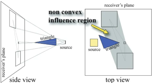
The influence region of a triangle is an overestimate of the union of the projections of the triangle from every point on the source. Since the goal is to consider all points poten-tially influenced, a bounding region suffices. Because source and triangles are convex, the influence region is contained in the convex hull of the projections of the triangle from the corner of the source. Note that it is only contained if one considers a one-sided triangle, as shown on Fig.1. Instead of computing the convex hull, which is quite involved, we conservatively bound it by an axis-aligned bounding box. It is computed from the triangle using a geometry shader. We pass as uniform parameters the 4 matrices of the projections on the receiving plane from the source’s corners. For plane ax+ by + cz + d = 0 and corner (u,v,w), the matrix is given by:
M:= [abcd] × [uvw1]T− (au+ bv + cw)I (3) c
E. Eisemann& X. Décoret / Preprint: Visibility Sampling on GPU source triangle triangle receiver’s plane receiver ’s plane source non convex influence region
side view top view
Figure 1: For a one-sided convex caster (blue triangle) and a convex source (yellow square) the convex hull is not the best overestimate that can be constructed from the vertices.
The geometry shader receives the triangle’s vertices, projects them using the matrices, computes an axis-aligned bounding box of the obtained 4 × 3 vertices, and outputs it as a quad.
4. Backprojections on light source
For each point in the influence region, we find which part of the source is hidden by the triangle by backprojecting it onto the source. This backprojection can be interpolated from the backprojections of the vertices of the triangle’s influence region. This is possible because it is a projective applica-tion. We compute these in the geometry shader using eq. (3) again, and pass them to the fragment shader as three inter-polated texture coordinates. Note that this time, the back-projection matrix depends on the triangle, and should there-fore be built in the geometry shader, not passed as a uni-form. Coordinates of the backprojected triangle are com-puted in normalized source frame where the source is the square x= ±0.5,y = ±0.5,z = 0. At this stage, summarized
P
T Receiver
’s plane
Source
Conservative influence region of T
Backprojection of T from P Projection of T from source's corner
Figure 2: Overview of how our approach finds the region blocked by a triangle. A geometry shader computes an over-estimate of the true influence region. A fragment shader com-putes the backprojection and hidden samples.
on Fig.2, we produce fragments that correspond to points inside the triangle’s influence region and that have access,
through three texture coordinates, to the backprojection of the triangle. The next step is to find which source samples fall in these backprojections.
5. Samples inside backprojection
To encode which samples are inside/outside a backprojec-tion, we use a 32 bit bitmask encoded as RGBA8 color, that is 8 bits per channel. Our fragment shader will then output the sets of blocked samples as the fragment’s color. Computing which samples are inside the backprojection can be done by iterating over the samples, but would be very inefficient. Since the set of samples inside a 2D triangle is the intersection of the set of samples on the left of the supporting line of each (oriented) edge, we can devise a better method based on precomputed textures, in the spirit of [KLA04]. An oriented line in the 2D plane of the normalized source frame can be represented by its Hough transform [DH72], that is an angle θ ∈ [−π, π] and a distance r to the gin. The distance can be negative because we consider ori-ented lines. However, we need only those lines that intersect the normalized light square so we can restrict ourselves to r ∈[−
√ 2/2,+
√
2/2]. In a preprocess, we sample this Hough space in a 2D texture called the bitmask texture. For ev-ery texel (θ, r), we find the samples located on the left of the corresponding line and encode them as a RGBA8 bit-mask (Fig.3, left).
At run-time, our fragment shader evaluates which samples lie within the backprojection as follows. We first ensure the backprojection is counter-clockwise oriented, reversing its vertices if not. Then the lines supporting the three edges of the backprojection are transformed into their Hough coor-dinates, normalized so that [−π, π] × [−
√
2/2,+√2/2] maps to [0, 1] × [0, 1]. These coordinates are used to look-up the three bitmasks encoding which samples lie on the left of each edge. The Hough dual is periodic on θ, thus we use the GL_REPEAT mode for it and GL_CLAMP for r. The latter correctly gives either none or all samples for lines not inter-secting the normalized light square. These three bitmasks are AND-ed together to get one bitmask representing the sam-ples inside the backprojection. This result is output as the fragment’s color (Fig.3, right).
Performing a bitwise logical AND between three values in the fragment shader requires integer arithmetic. This feature is part of DirectX10, and is implemented only on very re-cent graphic cards. However, if not available, it can be em-ulated [ED06a] using a precomputed 2563texture such that:
opMap[i, j, k]= i AND j AND k (4) Then, to perform the AND between three RGBA8 values ob-tained from the bitmasks texture, we just do a 3D texture lookup to AND each of the channels together. This approach c
( 1,1 +1 -1 +1 -1 0,0 1 1 1 0 0 0 1 1 1 0 0 1 1 1 1 1 1 1 1 1 1 1 1 1 1 1 1 1 1 1 1 1 r r r θ θ θ
Light normalized square
bitmasks texture GL_REPEAT R G B A GL_CLAMP oriented line (a) (b) (c) (d) left of C inside ABC left of B left of A A C B bitwise AND (a) (b) (c) 1 1 1 1 1 1 1 1 1 1 1 1 1 1 1 1 1 1 1 1 1 1 1 1 1 1 1 1 1 1 1 1 1 1 1 1 1 1 1 1 1 0 1 0 1 1 1 1 1 1 1 1 1 1 1 1 0 1 1 1 1 1 0 1 1 1 0 1 1 1 1 1 1 0 1 0 1 1 0 1 1 1 1 1 1 1 1 1 0 0 1 0 1 1 0 1 1 1 0 1 1 1 1 1 1 1 1 1 1 1 0 1 1 1 1 1 1 1 1 1 1 0 1 0 1 1 1 1
Figure 3: (left) Pre-processing the bitmask texture for a set of 32 samples. For every texel (θ, r) we build the line corresponding to this Hough space value (a) and find the samples located on the left of it (b). These samples are encoded as a bitmask (c) that we cast as the RGBA8 color of the texel (d). The sine wave in the resulting textures corresponds to the Hough dual of the sample points. (right) To find the light samples within the backprojection of a triangle (a), we use the bitmask texture. We look-up bitmasks representing the samples lying on the left of each edge (b) and combine them using a bitwise AND (c).
is general: any logical operation can be evaluated using the appropriate opMap texture.
5.1. Combining the occlusion of all triangles
The set output by the fragment shader for a receiver sample Rjand a triangle Tkcan be formally written as :
Bj,k≡nisuch as [Si,Rj] ∩ Tk, ∅ o
(5) To compute the Bj, we use the fact that Bj= SkBj,k. With our bitmask representation, the union is straightforward. All we have to do is to OR the colors/bitmasks of each fragment incoming at a same location. This is done automatically by the graphics card by enabling the logical operation blending mode. The resulting image is called hidden-samples map. 6. Sampling considerations
Our algorithm treats the source and the receiver asymmet-rically. The source is explicitly sampled. The samples can be arbitrarily positioned using regular or irregular patterns. All that is required is to compute the bitmasks texture for the chosen pattern. Conversely, The receiver is implicitly sam-pled. The rasterization of the influence regions implies that the Rjare at the center of the texels of the hidden-samples map. The samples are regularly placed, and their number is given by the texture resolution. Using a 512 × 512 yields about 262k samples, which is much higher than the 32 on the source. Finally, the resulting hidden-samples map indi-cate which part of the source is not visible from receiver points. To get the opposite information – which part of the receiver a source point sees – it only has to be inverted. Depending on the context, this asymmetry may not be a
problem. It can always be alleviated by performing two passes, switching the source and receiver. In subsequent sec-tions, we discuss how we can improve the number of sam-ples, and the quality of the sampling.
6.1. Increasing source samples
We described the algorithm with 32 samples on the source because it is the number of bits available in a typical OpenGL color buffer. Recent cards support buffers and tex-tures with 4 channels of 32 bits each, leading to 128 samples in theory. In practice, when using an integer texture format, only 31 bits can be used because of reserved special values. Thus, we can treat 124 samples.
Of course, the number of samples can be increased using multiple renderings, but the benefit of the single pass nature would be lost. We use Multiple Render Targets (MRT), a feature of modern graphic cards that lets fragment shaders output up to eight fragments to separate buffers. Thus, it is possible to evaluate up to 992 samples in a single rendering pass pass by rendering eight hidden samples maps.
6.2. Decorrelating source samples
If there are particular alignments of the scene and the light, or for large sources, a fixed sampling may become visible, even with 128 samples. To alleviate this problem, one can vary the set of samples for each receiving point. We just need to slightly perturb the positions of the backprojections by a random amount based on the position on the receiving plane. We use: random(x, y)= frac(α(sin(βy ∗ x) + γx)) which pro-duces a reasonably white noise if α, β, γ are correctly chosen depending on the texture resolution.
c
E. Eisemann& X. Décoret / Preprint: Visibility Sampling on GPU 1 0 0 1 1 0 1 1 1 0 0 1 1 0 1 1 0 1 0 0 0 0 0 1 1 0 0 0 1 0 1 0 1 0 0 0 1 0 1 0 27 26 25 24 23 22 21 20 1 0 1 0 1 1 0 0 0 0 1 0 0 1 1 0 0 0 0 0 1 0 1 0 = 5 bits in initial bitmask initial bitmask 0 1 0 1 0 1 1 0 0 0 0 1 0 0 1 0 0 0 1 0 0 0 1 0 1 0 0 0 1 0 0 0 + 0 0 0 1 0 0 1 1 0 0 0 0 0 0 1 1 0 0 0 0 0 0 1 0 0 0 1 0 0 0 0 0 + +
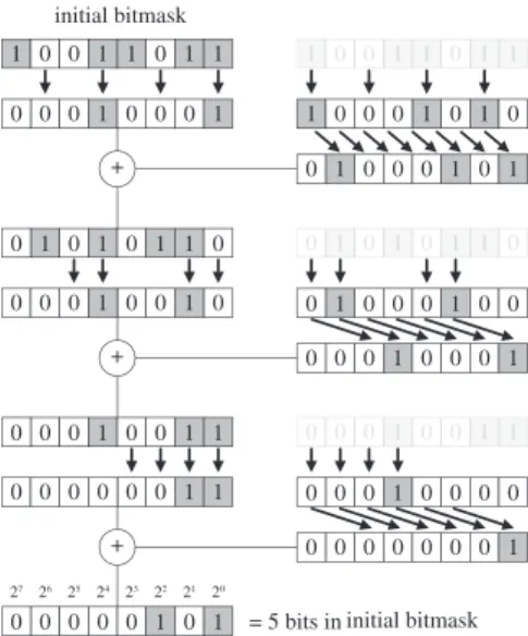
Figure 4: Counting bits in logarithmic time.
7. Backface culling
If the caster is watertight i.e. it encloses a volume, we can ignore every triangle that is front-facing for all points on the light source. Indeed, a ray blocked by such a triangle is nec-essarily blocked by a non-frontfacing one (it must enter and exit the volume). Culling the front faces is more interesting than culling the back faces, because it yields smaller influ-ence regions. In the geometry shader, we test if the triangle is front-facing by checking if it is front-facing for the four corners of the light source. If yes, it is safe to let the geom-etry shader discard it. This optimization eliminates roughly half the faces, and thus doubles the framerate.
8. Application to soft shadows
We can use our method to compute the soft shadows caused by an area light source on a receiving plane. Once we have computed the hidden-sample map, we convert it to a shadow intensity texture. This is done in a second pass, rendering a single quad covering the viewport and activating a fragment shader that does the conversion. The shader fetches the hid-den sample bitmask for the fragment, and counts how many bits are at 0. This can be done using a loop over bits, or a pre-computed texture [ED06a]. We use another method, whose complexity is logarithmic in the number of bits. We dupli-cate the bitmask, zero-ing odd bits in the first copy, and even bits in the second. We shift the second copy and add it to the first. We repeat the process log2(n) times to get the result Figure4illustrates the principle. More details can be found in [And].
Finally, we render the receiver texture-mapped with that tex-ture, using linear interpolation and mipmapping. Alterna-tively, we can do bit counting directly while rendering the
receiver. This is particularly interesting if the influence re-gions were projected from the receiving plane into the cur-rent view. In this case no aliasing occurs.
Our approach works correctly for very large sources, where many methods would fail due to the approximation of sil-houette edges from the center of the source. An approach like [HPH97] would require many samples, or aliasing ar-tifacts become noticeable. In our approach, we can decor-relate the sampling (see Section6.2) and trade aliasing for noise. Figure5shows the improvement. Decorrelating
sam-Figure 5: Decorrelating source sampling for each receiver point produces noisier but less aliased shadows. Here, only 32 light samples are used with a1024 × 1024 texture. The door is slightly above the ground, to better show the shadow.
pling has also been proposed in a more general framework
in [SIMP06].
Methods like [AHL∗06] are restricted to rectangular light sources. Our approach can handle any planar light source. We find a bounding rectangle, so we can compute backpro-jections from its corners, and place the samples where there is light. This can be very handy to compute shadows for neon-like sources where there are typically several long and thin tubes inside a square. It is also possible to use color-textured light sources. We pass to the shader the number of different colors, an array of color values, and an array of bit-masks indicating which samples are associated to each color. Then the shader counts bits in each group as before, multiply by the group color, and sum the result. In our implementa-tion, we organize samples so that the bits inside a texture channel corresponds to samples of the same color, so we do not need to pass group bitmasks. Using 8 MRTS, we can have up to 24 different colors, which is usually sufficient, and incur a negligible extra cost. Fig.6shows an example of a colored shadow.
Although we described our algorithm with a planar receiver, it can be adapted to handle a bumpy one. The backprojection of the triangle can be done in the fragment shader (instead of computing it in the geometry shader, and interpolating it for fragments, as described earlier). Thus, we can offset the frag-ment’s world position, for example looking up a height map (this requires that the receiver is a heightfield as seen from c
Light Texture
Config.
(a) (b) (c) (d)
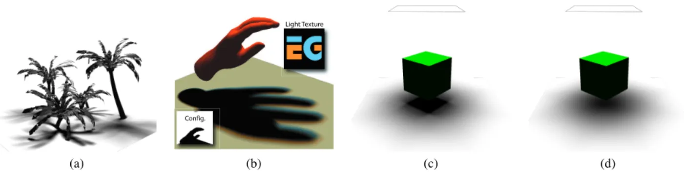
Figure 6: (a) An example of shadows using our method (b)Soft shadows caused by a textured light source, using 2 different colors. Notice the complex shadowing effect. The bottom left inset shows the source/receiver/scene configuration (c) A difficult case handled robustly by our method. Approximating shadows based on silhouettes from the center causes incorrect shadows (d). For moving light sources this approximation also causes strong popping.
at least one point of the source). As a result, we generate ac-curate soft shadows with high sampling rates for non-planar receivers, which has not been achieved before at interactive rates. Figure7shows an example. Some care must be taken 512 x 512 Bitmask, 4 MRT
20 fps (right) and 80 fps (middle)
Figure 7: Soft shadows on a non-planar receiver.
though. To assure conservative influence regions the projec-tion from the light’s corners (Secprojec-tion3) has to be performed on a plane lying behind the receiver. A (general) backprojec-tion is a costly operabackprojec-tion. Performing it in the fragment – not the vertex – shader can seriously affect the performance. If the receiver and source planes are parallel, which is a natu-ral choice when using a heightfield, the backprojection has a very simple expression.
We first compare with the method by Assarson et al. [AAM03,ADMAM03]. Their algorithm has two major shortcomings. First, only edges that are silhouettes for the center of the light are considered. This leads to temporal in-coherences, and inaccurate soft shadows as seen on Figure6. The additive combination of occluders leads to unrealistic umbra regions (in particular, it affects the penumbrae gra-dient). Figure8compares our method in such a situation. Furthermore our result is accurate (up to the sampling), so no temporal artifacts can be observed.
This said, our method has several drawbacks. It sepa-rates the caster from the receiver. It computes shadows on a planar (possibly bumpy) receiver, like some recent ap-proaches [AHL∗06]. Consequently, it is probably not suited
SSV Our SSV Our
Figure 8: Even for typical game characters, classical ap-proximations (silhouette from the center, additive occlusion) can cause noticeable artifacts. Here, it overestimates the umbra region. In comparison, our algorithm has no such approximation, and produces faithful results. In particular, there are no temporal incoherences when the light moves.
to applications like video games, and would be more inter-esting for fast previsualisation during the creation of static lightmaps. We insist that not shadow rendering, but visi-bility sampling, and the possibilities opened up by bitwise arithmetics are in the focus of the paper. Soft shadows just illustrate a possible use. Other tasks also benefit from our method, as demonstrated in the next application.
9. Application to assisted visibility edition
In video games, it is very important to guarantee that the framerate never drops below a certain threshold. For exam-ple, levels are often designed in a way that level-of-detail switches are not visible, or that many complex objects are not seen together from the current viewpoint. Most of this is anticipated during the design phase. Yet, the scene often needs to be modified afterwards. Typically, beta testers re-port where the game slowed down. Then the artist moves around objects a little, or add some dummy occluders to re-duce complexity. It is interesting that some elements of decor are added just to block the player’s view.
Visibility is not only a performance concern. It is often im-c
E. Eisemann& X. Décoret / Preprint: Visibility Sampling on GPU B C A 1 2 3
B
C
A
1
2
3
Figure 9: Interactive visibility visualisation: a designer can navigate a scene, place any two patches, and immediately (about 20Hz) see the unblocked rays joining the patches. Here, we show two such shafts (yellow). Closeups emphasize how well our method captures visibility, even for small features like the leaves (2) of the plant. See accompanying video for a demo.
portant to enforce that some objects remain invisible, while the player is following a certain path in the game. If guards could be killed from a distance a long time before they are actually supposed to be encountered, the gameplay would be seriously altered. Here again, tools to interactively visualize visibility could help designers preventing such situations. With our method, it is possible to place two rectangular re-gions in a scene, and immediately get information concern-ing their visibility. In particular, unblocked rays are returned (reading back the hidden-samples map). This information can be used to decide where to place objects to obstruct the view between the areas. The algorithm for soft shadows can be used to calculate an importance map indicating most vis-ibleregions. Accumulation over time is possible and allows to investigate the impact of moving objects.
We implemented such a system to visualize unblocked rays between two patches (Figure 9). We use 32 × 32 samples on source and receiver, which amounts to 1M rays consid-ered. Yet, it is very fast, even for complex scenes. The apart-ment model we used has approximately 80.000 triangles, and a complex instantiation structure. A thousand renderings (Heckbert-Herf’s approach) takes several seconds. With our method, we achieve about 20 fps, including a naive (ineffi-cient) ray visualisation, which provides interactive feedback to an artist designing a scene. She can edit the scene in real-time, and adapt it to control the desired visibility. Note that our method scales extremely well with geometry in this con-text. In particular it inherently performs shaft-culling: when a triangle is outside the shaft, the influence region calculated by our geometry shader is outside the NDC range. It is thus clipped and produces no fragments.
The fact that we can consider many rays per second largely
compensates the inherent inexactness of sampling. Interest-ingly, the visualization takes up more GPU resources than the determination of visibility. We compared the amount of rays per second with state-of-the-art ray-tracing approaches. Wald et al. describe a fast method to perform ray-tracing for animated scenes [WIK∗06]. The reported timings (on a dual core Xeon 3,2GHz processor) for intersection tests are 67Hz for a 5K model, 36Hz for a 16K and 16Hz for a 80K model, using a viewport of 10242pixels, which amounts to 1M rays. Our approach does not perform ray-tracing (intersections are not retrieved), but in term of speed, it achieves very high performance (see section10), is simpler to implement than a complete ray-tracing system and runs on an off-the-shelf graphics cards. Our approach works seamlessly with GPU based animation, skinning or geometric refinement. It is ex-ecuted completely on the GPU, leaving the CPU available to perform other tasks aside. Finally it would even be possible to combine typical ray-tracing acceleration techniques (e.g. frustum culling) with our approach.
10. Results& discussion
We made various measurements comparing our method with a multiple rendering approach [HPH97] on a P4 3000MHz. To allow for a fair comparison, we implemented a modified version of Heckbert and Herf’s algorithm. We rasterize di-rectly into a luminance texture using alpha blending and a stencil test (similar to [Kil99,Bli88]) instead of using the ac-cumulation buffer. This requires blending on float textures, which is available on latest cards. This modified implemen-tation is about 10 times faster (for 1000 samples) than the original accumulation buffer version.
Figure10shows the light’s influence. Our method is fillrate c
0.1 0.2 0.3 0.4 0.5 0.6 0.7 0.8 0.9 1.0 400 300 350 250 200 150 50 0 ms 100
Light size / scene radius HH 512/8 HH 256/8 HH 128/8 HH 64/8 Our 512/8 Our 256/8 Our 128/8 Our 64/8 0.1 0.2 0.3 0.4 0.5 0.6 0.7 0.8 0.9 1.0
Light size / scene radius ms 50 70 40 30 20 10 0 60 80 90 HH 512/8 HH 256/8 HH 128/8 HH 64/8 Our 512/8 Our 256/8 Our 64/8 Our 128/8 1.0 0.9 0.8 0.1 0.2 0.3 0.4 0.5 0.6 0.7 700 500 600 400 300 200 100 0
Light size / scene radius ms HH 512/8 HH 256/8 HH 128/8 HH 64/8 Our 512/8 Our 256/8 Our 128/8 Our 64/8 8 1 2 3 4 5 6 7 250 150 200 100 50 0 ms nb * 124 samples HH 256 Our 256
Figure 10: Compared influence of light and texture size for Heckbert& Herf(HH) and our method and 992 samples (8 MRT). Top left: palm trees (29 168 polys). Top right: bull (here 4000 tris). Bottom left: office (1700 tris). X-axis indicates light size with respect to scene radius. Y-axis reports rendering time (ms). Bottom right: sampling against computation time for the palm tree scene (top left) with a light/radius ratio of 0.4. For our method, more samples have almost scene independent cost.
limited. The larger the source, the larger the influence region and the slower the method becomes. On the contrary, Heck-bert’s method is independent of the sample’s location, hence the size of the source. For a giant source, it would however create aliasing that our method would address (see Figure5). We have really pushed our algorithm, since we considered very large sources (up to the size of the model), very close to the object. Yet, our method behaves better for sources up to half the scene radius. For the bull model, we activated the watertight optimization (Section7). This is why the per-formance drops more strongly than for the palm tree, where it was deactivated. When the source is very large, there are fewer and fewer fully front-facing polygons.
The bottom curves of Figure10are surprising at first: our method performs much better than Heckbert and Herf. Be-cause the result is obtained in a single pass, we apply ver-tex computations (transform, skinning, etc.) once. Real-life scenes, like the office, often contain objects instantiated sev-eral times with different transformations. This causes many CPU-GPU transfers of matrices, context switches, etc. that imped the performance when rendering the scene hundreds of time. The mere polygon count is not a sufficient criterion.
There are other factors that influence the performance of our approach, which therefore depends strongly on the type of scene. A small triangle close to a large source has a very large influence region. Since we treat each triangle indepen-dently, highly tesselated models incur a high overdraw and a performance drop. A natural solution is to perform mesh simplification on such models, and to use the result, which has less triangles. This is not just natural, it also makes sense. As pointed in [DHS∗05], high frequencies are lost in the presence of large light sources. The simplified model, even when very coarse, cast shadows that closely matches the ex-act one, as shown on Figure11. This improves rendering time, as shown on Figure12.
Note that it makes sense to compare the polygon count of different versions of the same object. Across models, it is ir-relevant: The palm tree scene has 30k polygons but since the leaves are small, they have relatively small influence regions and cause less fillrate than the 4k polygons of the bull model. One feature of our algorithm is that there are no real degen-eracies. It always works, up to the precision of the Hough sampling. Special cases, e.g. if the triangles intersect the receiver, can be solved by transporting the backprojection
c
E. Eisemann& X. Décoret / Preprint: Visibility Sampling on GPU
1000 Polys
Our
8000 Polys
Our
8000 Polys
Ref.
Figure 11: Our method delivers faithful visibility results. One major cost factor is the fillrate. It becomes expensive in the case of big sources due to overdraw. Interestingly these configurations represent exactly those, where a coarse model (left) would provide almost the same shadow. Therefore fillrate can be reduced drastically via simplification.
ms 0.1 0.2 0.3 0.4 0.5 0.6 0.7 0.8 0.9 1.0 25 30 20 15 10 5 0
Light size / scene radius HH256/8/500 HH256/8/1000 HH256/8/2000 HH256/8/4000 Our256/8/500 Our256/8/1000 Our256/8/2000 Our256/8/4000
Figure 12: Rendering time (ms) vs. nb polygons (bull model). X-axis indicates the size of the light source. The dif-ferent curves indicate difdif-ferently simplified versions.
to the fragment shader (as for the bumpy ground). Alterna-tively, the geometry shader could retriangulate the intersect-ing triangles. We want to outline that most results in this pa-per have been computed with relatively large sources, very close to the caster, which is a worst-case scenario for most other methods. Yet, it works well, even for notably difficult cases such as for the cube in Figure6.
11. Conclusion& future work
We presented a fast GPU based visibility algorithm, that samples equivalent to ray-tracing without much CPU work, but is much simpler to implement and faster (512 × 512 × 1000 samples ≈ 260M rays). Of course, ray-tracers are much more general). We believe it demonstrates the benefits of bit-wise arithmetic on modern GPUs, whose interest has already been shown in [ED06a].
We presented two possible applications illustrating the
util-ity of our method. The soft shadow application – although providing accurate real-time shadows on non-planar re-ceivers for the first time – should be seen as a proof of concept. It is probably not suited for games where realism is unnecessary. It can be useful though for fast computa-tion of lightmaps. The visibility edicomputa-tion is a novel applica-tion. Its strength is its speed and the ability to provide un-blocked rays. It can be implemented easily and does not in-terfere with any GPU technique (geometry encoding, skin-ning, etc.). The information read-back is inexpensive, due to the small texture size.
There exist various possibilities for future work. We would like to combine our method with algorithms like [NB04] to compute PVS. We are also interested in using it to speed up form factor estimation in hierarchical radiosity ap-proaches [SP94]. Finally, we are working on improvements of our soft shadow computations. Inspired by [DHS∗05], we can group triangles based on their distance to the source. The closer groups could be rendered in low resolution textures, and the furthest one in high resolution textures, thus reducing fillrate and improving speed. For globally cast shadows, we can compute shadow intensity on several parallel receivers, and interpolate in between, in the spirit of [ED06b]. Acknowledgements Special thanks go to U. Assarson for his help with the comparison. We thank Espona & Stanford for the models and L. Boissieux for the studio model. We further acknowledge the reviewers for their insightful com-ments and H. Bezerra for her help and suggestions.
References
[AAM03] A U., A-M¨ T.: A geometry-based soft shadow volume algorithm using graphics hard-ware. ACM Transactions on Graphics (Proc. of SIG-GRAPH 2003)(2003).
[ADMAM03] A U., D M., M M., c
A-M¨ T.: An optimized soft shadow vol-ume algorithm with real-time performance. In Proc. of the ACM SIGGRAPH/EUROGRAPHICS Workshop on Graphics Hardware(2003), ACM Press.
[AHL∗06] A L., H N., L M., H- J.-M., H C., S F.: Soft shadow maps: Efficient sampling of light source visibility. Computer Graphics Forum 25, 4 (dec 2006).
[AM04] A T., M V.: dpvs: An occlusion culling system for massive dynamic environments. IEEE Com-puter Graphics and Applications 24, 2 (2004), 86–97. [And] A S. E.: Bit twiddling hacks. graphics.
stanford.edu/~seander/bithacks.html.
[ASVNB00] A´ C., S-V´ C., N I., B P.: Integrating occlusion culling with levels of de-tail through hardly-visible sets. In Comp. Graphics Forum (Proc. of Eurographics)(2000), vol. 19(3), pp. 499–506. [Bli88] B J. F.: Me and my (fake) shadow. IEEE
Com-puter Graphics and Applications 8, 1 (1988), 82–86. [BWPP04] B J., W M., P H.,
P- W.: Coherent hierarchical culling: Hardware occlu-sion queries made useful. Computer Graphics Forum 23, 3 (Sept. 2004), 615–624.
[COCSD02] C-O D., C Y., S C., D- F.: A survey of visibility for walkthrough applica-tions. IEEE Trans. on Visualization and Comp. Graphics (2002).
[DDS03] D´ X., D G., S F.: Erosion based visibility preprocessing. In Proceedings of the Eu-rographics Symposium on Rendering(2003), Eurograph-ics.
[DDTP00] D F., D G., T J., P C.: Conservative visibility preprocessing using extended pro-jections. In Proc. of SIGGRAPH’00 (2000), pp. 239–248. [DH72] D R. O., H P. E.: Use of the hough trans-formation to detect lines and curves in pictures. Commun. ACM 15, 1 (1972), 11–15.
[DHS∗05] D F., H N., S C., C E., S F.: A frequency analysis of light transport. ACM Transactions on Graphics (Proceedings of SIGGRAPH 2005) 24, 3 (aug 2005). Proceeding.
[ED06a] E E., D´ X.: Fast scene voxelization and applications. In Proc. of I3D’06 (2006).
[ED06b] E E., D´ X.: Plausible image based soft shadows using occlusion textures. In Proceedings of the Brazilian Symposium on Computer Graphics and Image Processing, 19 (SIBGRAPI)(2006), Oliveira Neto Manuel Menezes deCarceroni R. L., (Ed.), Conference Series, IEEE, IEEE Computer Society.
[HMN05] H D., M O., N S.: A low
dimensional framework for exact polygon-to-polygon oc-clusion queries. In Rendering Technqiues 2005: Proceed-ings of the 16th symposium on Rendering(2005), Euro-graphics Association, pp. 211–222.
[HPH97] H S., P, H M.: Simulating Soft Shadows with Graphics Hardware. Tech. Rep. CMU-CS-97-104, Carnegie Mellon University, 1997.
[Kil99] K M. J.: Improving shadows and reflec-tions via the stencil buffer. NVidia white paper http: //developer.nvidia.com/attach/6641, 1999.
[KLA04] K J., L J., A T.: Hemispheri-cal rasterization for self-shadowing of dynamic objects. In Proceedings of the 2nd EG Symposium on Rendering (2004), Springer Computer Science, Eurographics, Euro-graphics Association, pp. 179–184.
[LA05] L S., A T.: Hierarchical penumbra casting. Computer Graphics Forum (Proceedings of Eurographics ’05) 24, 3 (2005), 313–322.
[LSCO03] L T., S O., C-O D.: Ray space factorization for from-region visibility. ACM Trans-actions on Graphics (TOG) 22, 3 (2003), 595–604. [MAM05] M F., A L., M´ M.:
Coher-ent and exact polygon-to-polygon visibility. In Proc. of WSCG’2005(January 2005).
[NB04] N S., B E.: Hardware accelerated aggressive visibility preprocessing using adaptive sam-pling. In Rendering Technqiues 2004: Proceedings of the 15th symposium on Rendering(2004), Eurographics As-sociation, pp. 207–216.
[NBG02] N S., B E., G J.: Exact from-region visibility culling. In Proc. of the 13th Workshop on Rendering(2002), pp. 191–202.
[SIMP06] S B., I J.-C., M R., P´ B.: Non-interleaved deferred shading of interleaved sam-ple patterns. In Proceedings of SIGGRAPH/Eurographics Workshop on Graphics Hardware 2006(2006).
[SP94] S F. X., P C.: Radiosity and Global Illu-mination. Morgan Kaufmann Publishers Inc., San Fran-cisco, CA, USA, 1994.
[WIK∗06] W I., I T., K A., K A., P S. G.: Ray Tracing Animated Scenes using Coherent Grid Traversal. ACM Transactions on Graphics (2006), 485– 493. (Proceedings of ACM SIGGRAPH 2006).
[WWS00] W P., W M., S D.: Visi-bility preprocessing with occluder fusion for urban walk-throughs. In Proc. of EG Workshop on Rendering ’00 (2000), pp. 71–82.
[WWZ∗06] W P., W M., Z K., M S., H G., R A.: Guided visibility sampling. ACM Transactions on Graphics 25, 3 (7 2006), 494–502.
c