Science Arts & Métiers (SAM)
is an open access repository that collects the work of Arts et Métiers Institute of Technology researchers and makes it freely available over the web where possible.
This is an author-deposited version published in: https://sam.ensam.eu
Handle ID: .http://hdl.handle.net/10985/12049
To cite this version :
Pierre LEQUIEN, Gérard POULACHON, José OUTEIRO, Joël RECH - Hybrid
experimental/modelling methodology for identifying the convective heat transfer coefficient in cryogenic assisted machining - Applied Thermal Engineering - Vol. 218, p.500-507 - 2018
Any correspondence concerning this service should be sent to the repository Administrator : archiveouverte@ensam.eu
Accepted Manuscript
Hybrid experimental/modelling methodology for identifying the convective heat transfer coefficient in cryogenic assisted machining
P. Lequien, G. Poulachon, J.C. Outeiro, J. Rech
PII: S1359-4311(17)32697-2
DOI: http://dx.doi.org/10.1016/j.applthermaleng.2017.09.054
Reference: ATE 11111
To appear in: Applied Thermal Engineering
Received Date: 21 April 2017
Revised Date: 4 September 2017
Accepted Date: 11 September 2017
Please cite this article as: P. Lequien, G. Poulachon, J.C. Outeiro, J. Rech, Hybrid experimental/modelling methodology for identifying the convective heat transfer coefficient in cryogenic assisted machining, Applied Thermal Engineering (2017), doi: http://dx.doi.org/10.1016/j.applthermaleng.2017.09.054
This is a PDF file of an unedited manuscript that has been accepted for publication. As a service to our customers we are providing this early version of the manuscript. The manuscript will undergo copyediting, typesetting, and review of the resulting proof before it is published in its final form. Please note that during the production process errors may be discovered which could affect the content, and all legal disclaimers that apply to the journal pertain.
Hybrid experimental/modelling methodology for identifying the convective
heat transfer coefficient in cryogenic assisted machining
P. Lequien
1, G. Poulachon
1, J.C. Outeiro
1, J. Rech
21
Arts et Metiers, LaBoMaP, 71250 Cluny, UBFC, France
2
Univ Lyon, ENISE LTDS, CNRS UMR5513, 58 Rue Jean Parot, 42023 Saint-Etienne cedex 2, France
HIGHLIGHTS
Investigation of heat transfer coefficient between LN2 and titanium alloy
Influence of LN2 projection parameters on temperature distribution in the workpiece Determination of h (W/m².K) with temperature measurement and CFD simulations Results highly depends on LN2 projection parameters (pressure and nozzle diameter) Mathematical development for predicting convective heat transfer coefficient ARTICLE INFO
Article History:
Keywords:
Liquid nitrogen Cryogenic machining Convective heat transfer coefficient
Ti6Al4V
ABSTRACT
Cryogenic assisted machining has become a very popular method in the metal cutting industry, as it enables the cooling of a cutting zone for improving surface integrity or/and tool life without contaminating the machined part. However, the thermal interaction between liquid nitrogen (LN2) and a hot cutting zone remains
unclear. The main objective of this work is to analyse the thermal phenomena occurring at the LN2 jet/workpiece interface. The
nitrogen liquid/gas phase proportion has a significant influence on the heat transfer. To determine the influence of LN2 jet parameters
on the convective heat transfer coefficient, a model based on the projection of an LN2 jet on a workpiece instrumented with
thermocouples is proposed. The most influential parameters of the thermal distribution and heat transfer coefficient are LN2 pressure,
nozzle diameter, projection angle and the distance between the
nozzle and the workpiece surface.
1 INTRODUCTION
The heat generated during machining operations is particularly significant when cutting difficult-to-cut materials such as Ti6Al4V alloy because
of its poor thermal conductivity [1] and its high friction coefficient combined with strong adhesion [2]. Thus, tool wear is accelerated, and the surface integrity becomes deteriorated.
Venugopal et al. [3] observed tool wear reduction when turning a Ti6Al4V alloy under the application of LN2. Shokrani et al. [4]
discovered a 40% reduction in surface roughness (Ra) compared to dry turning under cryogenic
cooling. Although there is clear interest in the cryogenic assisted machining [5], the available publications reveal many contradictory results, such as an increase and decrease of the cutting forces and premature tool failure [6]-[7]. The reason for the discrepancies in these results can be interpreted as a lack of knowledge of the physical phenomena associated with cryogenic assisted machining. Therefore, it is important to study the thermal phenomenon associated with the interaction between LN2 fluid and
components of a cutting system (tools, chips and the workpiece).
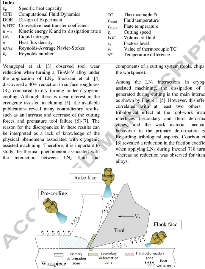
Among the LN2 interactions in cryogenic
assisted machining, the dissipation of heat generated during cutting is the main interaction as shown by Figure 1 [5]. However, this effect is correlated with at least two others: the tribological effect at the tool-work material interfaces (secondary and third deformation zones) and the work material mechanical behaviour in the primary deformation zone. Regarding tribological aspects, Courbon et al. [8] revealed a reduction in the friction coefficient when applying LN2 during Inconel 718 turning,
whereas no reduction was observed for titanium alloys.
Figure 1: Heat sources and application of the liquid nitrogen fluid
Index
Specific heat capacity
CFD Computational Fluid Dynamics DOE Design of Experiment
, HTC Convective heat transfer coefficient
Kinetic energy K and its dissipation rate ε LN2 Liquid nitrogen
Heat flux density
RANS Reynolds-Average Navier-Stokes Reynolds number
TCi Thermocouple #i Fluid temperature Plate temperature
Cutting speed
VOF Volume of fluid
Factors level
i Value of thermocouple TCi
Regarding the work material mechanical behaviour, authors consider that LN2 enables one
to reach the brittle fracture of the chip [9], which is said to facilitate chip fragmentation and increase cutting tool-life as a consequence. This paper focused on the thermal phenomenon occurring during the application of a LN2 jet
when machining Ti6Al4V titanium alloy. More precisely, it intends to model the h coefficient between a nitrogen fluid (mixture of liquid and gas) and a titanium part without any cutting process. The aim is to be aware about heat transfer phenomena occurring with LN2
projection on a workpiece. The temperature levels and convection coefficients are different to those really obtained during machining a refractory alloy. Many papers, such as Hong et al.’s study [10], have shown the importance of the nitrogen delivering strategy on cutting performances. The most efficient cooling strategies seem to be those where the nitrogen fluid is projected on the cutting and rake tool faces simultaneously, as shown in Figure 1. However, there is no quantitative explanation for the physical phenomena responsible for this evidence. Two question may arise. First, what is the applied LN2 flow rate? Second, which
liquid/gas ratio was present at the nozzle exit during such experiments (liquid/gas ratio)? It is well known that higher heat transfer is achieved by using a liquid phase when compared to a gas phase [11]. Thus, the objective is to keep the liquid/gas ratio as high as possible. Without a clear and comparable experimental set-up, it is impossible to optimize this technical solution or to transfer it to any other context.
To fix this problem, some papers have begun to identify the influence of the liquid/gas ratio on the heat transfer coefficient [5], [12], [13]. However, the identified coefficients exhibit a large deviation due to the large influence of the work material and test conditions. For instance, a value of approximately 5x10⁴ W/m².K was reported by Jawahir et al. [14] for cryogenic cooling during machining. Pusavec et al. [15] proposed a value of 2.5x10⁵ W/m².K, whereas
Hribersek [13] proposes an h coefficient of approximately 1.5x10⁴, which was determined by the inverse method based on cutting temperature measurement and numerical simulations. All of those values were determined by using several approaches. The condition of LN2 application was not considered and the ratio
between the liquid and the gas phase was not determined.
Empirical statements on the sensitivity of the nitrogen application strategy and the preliminary investigation on the h coefficient do not enable a clear scientific optimization of the LN2
application. There is a need for modelling of cutting operations under cryogenic assistance in order to optimize its thermal effects. This numerical simulation requires an accurate determination of the h coefficient in the vicinity of the cutting zones (Figure 1), i.e., in front of the tool edges (pre-cooling), on the rake face, on the flank face, etc. Numerical simulation intends to solve the balance between heat generated in various shear zones and cooling in various interfaces (work material and cutting tool). For a determined LN2 application, it can improve the
cutting conditions due to the corresponding h coefficient on each interface. However, it is necessary to know how the heat transfer coefficient will be affected when varying nitrogen pulverization conditions (ex: influence of the pressure). It requires an accurate model of the h coefficient depending on the application conditions such as nozzle diameter, pressure, distance, projection angle, etc. Based on such a model describing the influence of nitrogen projection conditions on heat transfer coefficients, it becomes possible to optimize the application strategy of the nitrogen and the corresponding cutting conditions.
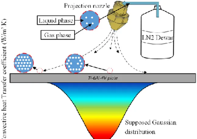
The ideal situation would be to propose a model of the entire phenomena occurring from the tank, as illustrated in Figure 2, to the work material interface. When reaching the nozzle, nitrogen is mainly, but not only, in a liquid phase. Then, the nitrogen mixture is projected into the air. A large variation of the liquid/gas ratio occurs during the
contact with air due to the rapid decrease of pressure and the rapid heating. Finally, the mixture comes in contact with the titanium plate. This area is usually very hot due to heat generated by cutting. The large difference of temperature between the nitrogen mixture and the surface induces boiling phenomena, known as the Leidenfrost effect [16], which strongly affects the heat transfer between the nitrogen mixture and the titanium alloy. It remains a scientific challenge to model such phenomena. The objective of the present work will mainly focus on the modelling of the nitrogen transfer between a nozzle and a titanium sample, as shown in Figure 2. This numerical model will be calibrated using an experimental setup in which the titanium plate is instrumented with thermocouples. This hybrid experimental-numerical approach will first enable one to determine the 3D distribution of coefficient h (W/m².K) on the surface for each nitrogen conditions, as illustrated in Figure 3. Then, by varying the nitrogen application conditions (pressure, nozzle’s diameter, distance, projection angle), it will be possible to determine the most sensitive parameter and to identify a global heat transfer coefficient density distribution model depending on nitrogen application conditions.
Figure 2: h coefficient distribution and evolution of the liquid/gas ratio
2 EXPERIMENTAL SETUP AND NUMERICAL MODEL
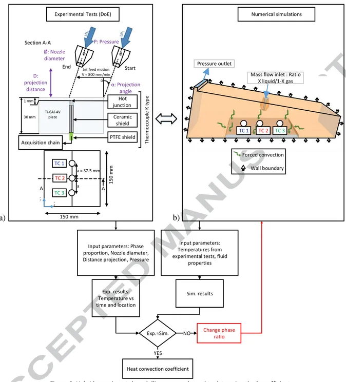
Figure 3a presents the experimental setup designed to measure the temperatures inside a Ti6Al4V plate during the projection of the nitrogen mixture. In parallel, an inverse approach based on numerical simulation in StarCCM+ has been developed to determine the h coefficient distribution, induced by a fluid nitrogen jet (Figure 3b). It also shows the experimental and numerical temperatures fit from thermocouples TC 1, TC 2 and TC 3. It is possible to estimate the parameters of the h coefficient distribution (Figure 3c). The liquid/gas ratio at the inlet nozzle is the fitting parameter to be adjusted.
Figure 3: Hybrid experimental-modelling approach used to determine the h coefficient 2.1 EXPERIMENTAL SETUP AND PARAMETERS
Figure 3a presents the experimental setup. A nozzle sprays the nitrogen flow onto a titanium workpiece (150 x 150 x 30 mm3) in which three calibrated, K type thermocouples are embedded with a 37.5 mm pitch. The hot junction is located on the flat bottom hole with a 1 mm controlled depth from the surface. The tank used for these tests is a 450 L capacity in which the pressure is manually controlled from 1.8 to 8 bars. The
nozzle is moved to the plate centre with an 800 mm/min constant speed. The levels of the four investigated factors are shown in Table 1.
Factors Level 1 Level 2
1 P: Pressure (bar) 2 6
2 α: Projection angle (°) 15 45
3 D: Distance (mm) 25 50
4 Ø: Nozzle diameter (mm) 1.5 3
Table 1: Design Of Experiments (DOE)
Mass flow inlet : Ratio X liquid/1-X gas Pressure outlet Forced convection Wall boundary α: Projection angle Ø: Nozzle diameter P: Pressure Acquisition chain Hot junction Ceramic shield PTFE shield Ti-6Al-4V plate 150 mm 150 mm
Jet feed motion V = 800 mm/min Ø Start Ø End α a a = 37.5 mm 1 mm TC 3 TC 2 TC 1 TC 3 TC 2 TC 1 x y Section A-A A A
Input parameters: Phase proportion, Nozzle diameter, Distance projection, Pressure
Exp. results: Temperature vs time and location
Heat convection coefficient
Input parameters: Temperatures from experimental tests, fluid
properties Sim. results Change phase ratio NO Exp.≈Sim. YES
Experimental Tests (DoE) Numerical simulations
30 mm a) b) Th erm o co u p le K t yp e D: projection distance
2.2 NUMERICAL MODEL AND PARAMETERS To understand the fluid mechanisms, phase proportion and the determination of the h coefficient induced by the LN2 projection on a
Ti6Al4V workpiece, a simulation has been
developed using StarCCM+ commercial
software. The main difficulty is the modelling of the correct fluid behaviour to reach the experimental temperature 1 mm beneath the sample/fluid interface considering the physical properties of LN2 (Table 2). The cooling rate is
measured by the thermocouples during the experimental test and applied at the same thermocouple positions in the numerical model. The CFD model is developed using a literature review which matches to this case [15]. Ameel et al. [17] established an analytical solution for the average h coefficient for turbulent flow. It allows one to determine coefficients of the K-ε turbulence model [18].
LN2 N2
Boiling point (°C) -196
Density (kg/m3) 807.3 1.15
Specific heat (J/kg.K) 2050 1041
Dynamic viscosity (mPa.s) 0.158 0.178 Thermal conductivity
(W/m.K)
0.1396 0.026 Table 2: Fluid properties [19]
Figure 3b shows the numerical model of the fluid projection on a plate, composed of three main domains: plate, nozzle and environment. Boundary conditions are presented. The nozzle inlet is considered as a mass flow inlet whereas the outflow is a pressure outlet. All the other boundaries of the model are assumed to be walls. The following assumptions were made:
The thermo-dependent properties of the materials are homogeneous and isotropic. The heat transfer modes are mainly
conduction and convection.
The heat flux should be a Gaussian-distributed in order to accelerate computation. It can be described as a reduced normal law. This model was meshed with two different methods. In one case, the plate was meshed with
470,000 tetrahedral elements. In the other case, the environment was meshed with 190,000 polyhedral elements. The mesh refinement was operated near critical regions where a strong temperature gradient may occur. The method of prism layer mesher was used to increase the accuracy between the fluid/wall interactions. In this case, the boundary layer was refined to capture physical phenomena, which may appear between the LN2 and the titanium plate. It is
mainly concerned with the Leidenfrost effect and fluids perturbations. The coefficient h
is
defined by Equation (1).
The resolution of the RANS (Reynolds Average Navier-Strokes) equation model [20] and Eulerian multiphase equations were used to simulate LN2 flow from the nozzle to the
workpiece [21]. It enables one to represent the wall-bounded turbulent flow. The use of Reynolds decomposition, applied to solutions of the Navier-Stokes equation, may simplify the problem by eliminating the fluctuations of short periods and amplitudes. The flow is considered to be turbulent (Re > 2500). The simulation
integrates the K-ε turbulence model in which transport equations are solved for the turbulent kinetic energy K and its dissipation rate ε. These constants are empirically derived. The transport equations are of the form suggested by Jones and Launder [22], with coefficients suggested by Launder and Sharma [23]. To comply with the liquid/gas nitrogen phase ratio, a VOF (Volume of Fluid) model is implemented in this simulation. These criteria will be optimized to correlate the experimental and numerical cooling rate. Fluid properties considered are described in Table 3 and model data input is listed in Table 4.
Fluid CMU C1e C2e Ct Σ k Σ e
LN2 0.09 1.44 1.9 1 1 1.2
Fluid
Fluid Inlet Initial temperature (°C)
-200 Turbulent dissipation rate (m²/s3) 0.2 N2 liquid/gas volume fraction 0.9
Turbulent viscosity ratio 10
Work material
Inlet Initial temperature (°C) 20
Titanium properties [24]
Table 4: Model data initial input 3 RESULTS AND DISCUSSION
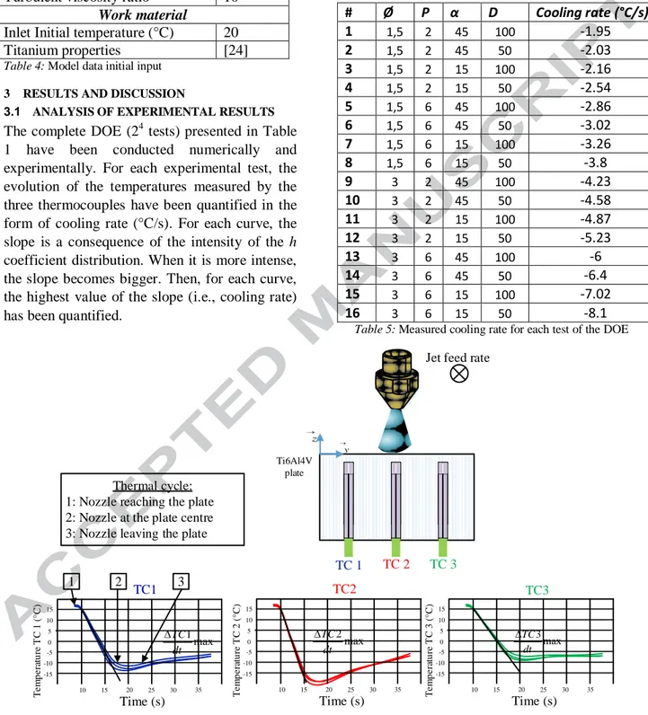
3.1 ANALYSIS OF EXPERIMENTAL RESULTS The complete DOE (24 tests) presented in Table 1 have been conducted numerically and experimentally. For each experimental test, the evolution of the temperatures measured by the three thermocouples have been quantified in the form of cooling rate (°C/s). For each curve, the slope is a consequence of the intensity of the h coefficient distribution. When it is more intense, the slope becomes bigger. Then, for each curve, the highest value of the slope (i.e., cooling rate) has been quantified.
Each experimental test, indicated in Table 5 and Figure 4, was performed three times, and the maximal cooling rate average was retained. It appears that the cooling rate varies between -1.95°C/s and -8.1°C/s. # Ø P α D Cooling rate (°C/s) 1 1,5 2 45 100 -1.95 2 1,5 2 45 50 -2.03 3 1,5 2 15 100 -2.16 4 1,5 2 15 50 -2.54 5 1,5 6 45 100 -2.86 6 1,5 6 45 50 -3.02 7 1,5 6 15 100 -3.26 8 1,5 6 15 50 -3.8 9 3 2 45 100 -4.23 10 3 2 45 50 -4.58 11 3 2 15 100 -4.87 12 3 2 15 50 -5.23 13 3 6 45 100 -6 14 3 6 45 50 -6.4 15 3 6 15 100 -7.02 16 3 6 15 50 -8.1
Table 5: Measured cooling rate for each test of the DOE
Figure 4: Evolution of the temperature measured by the three thermocouples and quantification of the average temperature
cooling rate from three tests for each experiment
Ti6Al4V plate TC 1 TC 2 TC 3 10 15 20 25 30 35 15 10 5 0 -5 -10 -15 Time (s) T e m p e ra tu re T C 1 (°C ) 10 15 20 25 30 35 15 10 5 0 -5 -10 -15 Time (s) T e m p e ra tu re T C 2 (°C ) 10 15 20 25 30 35 15 10 5 0 -5 -10 -15 Time (s) T e m p e ra tu re T C 3 (°C ) max 1 dt TC max 2 dt TC max 3 dt TC
Jet feed rate
Thermal cycle: 1: Nozzle reaching the plate 2: Nozzle at the plate centre 3: Nozzle leaving the plate
1 2 3 TC1 TC2 TC3 y z
3.2 SIMULATION RESULTS AND DETERMINATION OF THE CONVECTIVE HEAT TRANSFER COEFFICIENT The cooling rates derived from the experimental
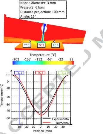
measurement were introduced into the simulation. The phase proportion was adjusted iteratively in order to obtain the predicted cooling rate and to fit with the experimental rate. It matched for a proportion of 90% liquid and 10% gas for all tests. Figure 5 presents a steady state simulation of the jet with thermal mapping. All numerical temperatures are extracted from the x longitudinal axe crossing the workpiece centre. It compares an example of the measured and predicted temperature distribution in the Ti6Al4V plate after the LN2 phase optimization.
Figure 5: Comparison between measured and predicted
temperature distribution in Ti6Al4V workpiece
When the optimization is completed, a difference between the measured and the calculated temperatures remains. This is due to the uncertainty in the thermocouple properties, and due to the numerical assumptions.
Finally, the distribution of the h coefficient in the plate is numerically deduced with StarCCM+ software. Figure 6 plots the chart for one similar test condition, as shown in Figure 5.
The Figure 6 represents the 3D plate with a maximum value on the centre and a cryogenic fluid impact that shows the maximal h coefficient. The plate dimensions are 150 mm x 150 mm. For a mind mapping, the three thermocouples experimentally used, are illustrated. It appears that the maximum heat transfer correspond to the thermocouples TC 2. At the plate’s edges, the heat transfer coefficient is greater than 0 W/m².C and not more than 200 W/m².K. This corresponds to the natural convection numerically imposed on the workpiece. This effect is trifling compared to the heat flux imposed by the cryogenic jet.
Figure 6: Surface heat transfer on Ti6Al4V workpiece A maximal value of this coefficient is observed at the plate’s centre, reaching 15,630 W/m².K. This value depends on the thermal difference between the fluid and the plate (Equation (1)). Temperature (°C) -202 -157 -112 -67 -22 22 Nozzle diameter: 3 mm Pressure: 6 bars Distance projection: 100 mm Angle: 15° TC 3 TC 2 TC 1 -30 -20 -10 0 10 20 30 10 0 -10 -20 -30 -40 -50 Experimental Numerical TC 1 TC 2 TC 3 Position (mm) Temp era tu re (°C ) Nozzle diameter: 3 mm Pressure: 6 bars Distance projection: 100 mm Angle: 15° x 104 1,5630 C onve cti ve he a t tr ans fe r coe ff icient (W /m ². K ) C onve cti ve he a t tr ans fe r coe ff icie nt (W /m ². K ) x 104 2.5 2 1.5 1 0.5 0 -0.5 50 0 -50 -50 50 0 2 1 0 Plate x dimension (mm) -20 0 20
All numerical simulations done in correlation with the design of experiments (Table 1) have been used to obtain the h coefficient.
The worst parameters in terms of convection heat transfer were obtained with: high projection angle, high projection distance, and low pressure associated with low nozzle diameter.
Coefficient h varies from 8,825 W/m².°C to 15,630 W/m².°C, depending on LN2 jet
parameters. Surface heat flux is influenced by boiling phenomena.
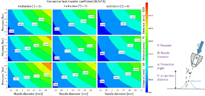
Regarding the 4D contour chart (plotted from a multi-linear regression model) presented in Figure 7, the nozzle diameter is the dominant parameter in response, which is directly correlated to the amount of LN2 reaching the
surface. The three next parameters are linked to the capacity to remain in a liquid state, which induces a much higher h coefficient [22]. The second most important parameter is the pressure. This parameter is linked to the contact time
between the LN2 and the surface, and with a high
pressure jet, the liquid phase may remain longer in the stagnation zone at the interface. In contrast, with a weak pressure jet, the stagnation zone cannot exist and the liquid is spread out and is transformed more rapidly into gas. The third important parameter is the projection angle of the cryogenic flow. As the projection angle is closer to the normal of the plate, the liquid phase interacts more rapidly with the work material. Finally, the distance is the least important parameter. As the distance decreases, the LN2
has less potential to transfer heat with its environment and as a consequence can remain in its liquid phase longer. The combination of these three parameters seems to be very dependent on each other.
In summary, it is possible to optimize the h between the nitrogen jet and the titanium plate when choosing a large nozzle diameter, a high pressure, a low distance and a jet orientation normal to the surface.
3.3 MODEL FOR PREDICTING THE
CONVECTIVE HEAT TRANSFER
COEFFICIENT
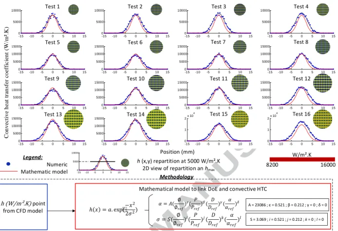
To obtain a simple equation that links the design of the experiments to the convective heat transfer coefficient, a methodology is suggested. The h coefficient deduced from the CFD model is plotted as a function of the position on the titanium plate, as shown by a blue point in Figure 8. These results are fitted with a non-normalized Gaussian curve with two parameters, which is presented by Equation (2) and a black curve on the same illustration.
The objective of this work is to identify the non-normalized Gaussian parameters ( and ) from the experimental factors ( . Two equations are established to determine each one with all experimental factors. Equations (3) and (4) show the type of chosen mathematical model.
The reference parameters of the mathematical model are named and and
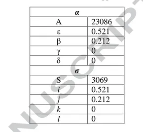
are arbitrary fixed with the respective values of 2 mm, 4 bars, 50 mm and 30 °. The Generalized Reduced Gradient method is used to solve this nonlinear constraint to obtain the value of the , β, γ, δ, i, j, k, l exponents and , coefficients. All of these coefficients are recapped in Table 6.
α A 23086 ε 0.521 β 0.212 γ 0 δ 0 σ S 3069 i 0.521 j 0.212 k 0 l 0
Table 6: Coefficient value of the mathematical model With this methodology, the maximum deviation with the experimental model is about 10% (test #16, Figure 8). A 2D section of the mathematical model was performed at 5,000 W/m².K in order to easily compare the h value and the repartition. The result is a gradient colour circle of each test.
Figure 8: Mathematical model methodology 4 CONCLUSION AND OUTLOOK
This paper presents the influence of LN2 jet
parameters on the temperature distribution of Ti6Al4V plate. It also proposes a methodology for determining the surface heat transfer coefficient between LN2 and the plate,
considering a multiphasic flow. It can be concluded that the liquid/gas phase proportion influences the depth of the cooling layer. The aim was to determine whether the cryogenic machining supply is sufficiently efficient as a cooling fluid. To understand thermal phenomena induced by this technology, an experimental and a numerical study was conducted to determine the h coefficient. The thermal response measured by the embedded thermocouples are greatly dependent on nozzle diameter, plate projection angle and LN2 pressure. To improve thermal
efficiency, high pressure and nozzle diameter may be considered. The experimental study shows that the optimization of the initial
parameters may increase the efficiency of cryogenic assistance.
In a second step, a numerical model was developed, and the predicted results were compared with those obtained experimentally. An inverse method was used to determine the convective convection heat flux using experimental temperature measurements. Using juxtaposition of the numerical and experimental curves, the phase ratio is adjusted. According to the obtained results, the following conclusions can be drawn:
The convective heat coefficient highly depends on experimental parameters. The nozzle diameter is the first parameter which influences cryogenic efficiency.
The value of the surface heat transfer between LN2 jet and Ti6Al4V plate can
reach 15,630 W/m².°C Coefficient convectif de transfert thermique :
Modele numerique et fit vs. Metamodele
H T C ( W /K .m ²) Position (mm) -15 -10 -5 0 5 10 15 0 1 2x 10 4 Essai 16 -15 -10 -5 0 5 10 15 0 1 2x 10 4 Essai 15 -15 -10 -5 0 5 10 15 0 5000 10000 15000 Essai 14 -15 -10 -5 0 5 10 15 0 5000 10000 15000 Essai 13 -15 -10 -5 0 5 10 15 0 5000 10000 15000 Essai 12 -15 -10 -5 0 5 10 15 0 5000 10000 15000 Essai 11 -15 -10 -5 0 5 10 15 0 5000 10000 15000 Essai 10 -15 -10 -5 0 5 10 15 0 5000 10000 15000 Essai 9 -15 -10 -5 0 5 10 15 0 5000 10000 15000 Essai 8 -15 -10 -5 0 5 10 15 0 5000 10000 15000 Essai 7 -15 -10 -5 0 5 10 15 0 5000 10000 15000 Essai 6 -15 -10 -5 0 5 10 15 0 5000 10000 15000 Essai 5 -15 -10 -5 0 5 10 15 0 5000 10000 Essai 4 -15 -10 -5 0 5 10 15 0 5000 10000 Essai 3 -15 -10 -5 0 5 10 15 0 5000 10000 Essai 2 -15 -10 -5 0 5 10 15 0 5000 10000 Essai 1 Legend: Numeric Mathematic model
Test 1 Test 2 Test 3 Test 4
Test 5 Test 6 Test 7 Test 8
Test 9 Test 10 Test 11 Test 12
Test 13 Test 14 Test 15 Test 16
Methodology
Position (mm)
h (x,y) repartition at 5000 W/m².K
2D view of repartition an hmax 8200 16000
W/m².K
h (W/m².K) point from CFD model
Mathematical model to link DoE and convective HTC
A = 23086 ; ε = 0.521 ; β = 0.212 ; γ = 0 ; δ = 0
S = 3.069 ; i = 0.521 ; j = 0.212 ; k = 0 ; l = 0
Coefficient convectif de transfert thermique : Modele numerique et fit vs. Metamodele
H T C ( W /K .m ²) Position (mm) -15 -10 -5 0 5 10 15 0 1 2x 10 4 Essai 16 -15 -10 -5 0 5 10 15 0 1 2x 10 4 Essai 15 -15 -10 -5 0 5 10 15 0 5000 10000 15000 Essai 14 -15 -10 -5 0 5 10 15 0 5000 10000 15000 Essai 13 -15 -10 -5 0 5 10 15 0 5000 10000 15000 Essai 12 -15 -10 -5 0 5 10 15 0 5000 10000 15000 Essai 11 -15 -10 -5 0 5 10 15 0 5000 10000 15000 Essai 10 -15 -10 -5 0 5 10 15 0 5000 10000 15000 Essai 9 -15 -10 -5 0 5 10 15 0 5000 10000 15000 Essai 8 -15 -10 -5 0 5 10 15 0 5000 10000 15000 Essai 7 -15 -10 -5 0 5 10 15 0 5000 10000 15000 Essai 6 -15 -10 -5 0 5 10 15 0 5000 10000 15000 Essai 5 -15 -10 -5 0 5 10 15 0 5000 10000 Essai 4 -15 -10 -5 0 5 10 15 0 5000 10000 Essai 3 -15 -10 -5 0 5 10 15 0 5000 10000 Essai 2 -15 -10 -5 0 5 10 15 0 5000 10000 Essai 1 C o n v ec ti v e h ea t tr an sf er c o ef fi c ie n t (W /m ². K ) = (∅∅ 𝑟 𝑓)(𝑟 𝑓) 𝛽( 𝑟 𝑓) 𝛾( 𝑟 𝑓) 𝛿 = ( ∅ ∅𝑟 𝑓) 𝑖( 𝑟 𝑓) 𝑗( 𝑟 𝑓) 𝑘( 𝑟 𝑓) 𝑙 = . exp( 2 2 2)
The numerical model highlights that the
jet reaching the plate surface is not only liquid. Phase transformation occurs and may also be modelled.
The phase ratio which most fits the experimental curves is 90% of LN2
The outlook of this work is to optimize the LN2
routing for cryogenic assisted machining to deliver the highest percentage of LN2 phase at
the cutting zone.
Acknowledgements
The authors would like to thank the Funds for Industrial Innovation (F2I), through the project reference, for financial support.
[1] C. Leyens and M. Peters, Eds., Titanium and titanium alloys: fundamentals and applications. Weinheim : [Chichester: Wiley-VCH ; John Wiley] (distributor), 2003.
[2] A. Egaña, J. Rech, and P. J. Arrazola, ‘Characterization of Friction and Heat Partition Coefficients during Machining of a TiAl6V4 Titanium Alloy and a Cemented Carbide’, Tribol. Trans., vol. 55, no. 5, pp. 665–676, Sep. 2012.
[3] K. A. Venugopal, S. Paul, and A. B. Chattopadhyay, ‘Growth of tool wear in turning of Ti-6Al-4V alloy under cryogenic cooling’, Wear, vol. 262, no. 9–10, pp. 1071–1078, Apr. 2007.
[4] Shokrani, V. Dhokia, S. T. Newman, and R. Imani-Asrai, ‘An Initial Study of the Effect of Using Liquid Nitrogen Coolant on the Surface Roughness of Inconel 718 Nickel-Based Alloy in CNC Milling’, Procedia CIRP, vol. 3, pp. 121–125, Jan. 2012.
[5] I. S. Jawahir et al., ‘Cryogenic manufacturing processes’, CIRP Ann. - Manuf. Technol., vol. 65, no. 2, pp. 713– 736, 2016.
[6] M. J. Bermingham, J. Kirsch, S. Sun, S. Palanisamy, and M. S. Dargusch, ‘New observations on tool life, cutting forces and chip morphology in cryogenic machining Ti-6Al-4V’, Int. J. Mach. Tools Manuf., vol. 51, no. 6, pp. 500–511, Jun. 2011.
[7] S. Y. Hong, I. Markus, and W. Jeong, ‘New cooling approach and tool life improvement in cryogenic machining of titanium alloy Ti-6Al-4V’, Int. J. Mach. Tools Manuf., vol. 41, no. 15, pp. 2245– 2260, 2001.
[8] C. Courbon, F. Pusavec, F. Dumont, J. Rech, and J. Kopac, ‘Tribological behaviour of Ti6Al4V and Inconel718 under dry and cryogenic conditions— Application to the context of machining with carbide tools’, Tribol. Int., vol. 66, pp. 72–82, Oct. 2013.
[9] N. R. Dhar, N. S. V. Kishore, S. Paul, and A. B. Chattopadhyay, ‘The effects of cryogenic cooling on chips and cutting forces in turning AISI 1040 and AISI 4320 steels’, Proc. Inst. Mech. Eng. Part B J. Eng. Manuf., vol. 216, no. 5, pp. 713–724, 2002.
[10] S. Y. Hong, ‘Economical and Ecological Cryogenic Machining’, J. Manuf. Sci. Eng., vol. 123, no. 2, p. 331, 2001.
[11] R. F. Barron, Cryogenic heat transfer. Philadelphia, PA: Taylor and Francis, 1999.
[12] F. Pusavec et al., ‘Analysis of the Influence of Nitrogen Phase and Surface Heat Transfer Coefficient on Cryogenic Machining Performance’, J. Mater. Process. Technol.
[13] M. Hriberšek, V. Šajn, F. Pušavec, J. Rech, and J. Kopač, ‘The Procedure of Solving the Inverse Problem for Determining Surface Heat Transfer Coefficient between Liquefied Nitrogen and Inconel 718 Workpiece in Cryogenic Machining’, Stroj. Vestn. - J. Mech. Eng., vol. 62, no. 6, pp. 331–339, Jun. 2016.
[14] I. S. Jawahir et al., ‘Cryogenic manufacturing processes’, CIRP Ann. - Manuf. Technol., vol. 65, no. 2, pp. 713– 736, 2016.
[15] F. Pusavec et al., ‘Analysis of the Influence of Nitrogen Phase and Surface Heat Transfer Coefficient on Cryogenic Machining Performance’, J. Mater. Process. Technol.
[16] J. G. Leidenfrost, De aquae communis nonnullis qualitatibus tractatus. Ovenius, 1756.
[17] T. A. Ameel, ‘Average effects of forced convection over a flat plate with an unheated starting length’, Int. Commun. Heat Mass Transf., vol. 24, no. 8, pp. 1113–1120, Dec. 1997.
[18] CD Adapco, StarCCM+ User Guide. 2014. [19] R. F. Barron, ‘Cryogenic treatment of metals to improve wear resistance’, Cryogenics, vol. 22, no. 8, pp. 409–413, Aug. 1982.
[20] W. K. George, ‘Lectures in Turbulence for the 21st Century’, Chalmers Univ. Technol., 2009.
[21] I. Demirdžić, S. Muzaferija, M. Perić, E. Schreck, and V. Seidl, ‘Computation of Flows with Free Surfaces’, in Scientific Computing in Chemical Engineering II, Springer, 1999, pp. 360–367.
[22] W. P. Jones and B. E. Launder, ‘The prediction of laminarization with a two-equation model of turbulence’, Int. J. Heat Mass Transf., vol. 15, no. 2, pp. 301–314, Feb. 1972.
[23] B. E. Launder and B. I. Sharma, ‘Application of the energy-dissipation model of turbulence to the calculation of flow near a spinning disc’, Lett. Heat Mass Transf., vol. 1, no. 2, pp. 131–137, Nov. 1974.
[24] B. Baudouy, G. Defresne, P. Duthil, and J.-P. Thermeau, ‘Propriétés des matériaux à basse température’, Tech. Ing. Froid Cryogénie Appl. Ind. Périphériques, vol. base documentaire : TIB596DUO., no. ref. article : be9811, 2014.