Model-based decoupling control method for dual-drive gantry stages : A case study with experimental validations

Science Arts & Métiers (SAM)

is an open access repository that collects the work of Arts et Métiers Institute of Technology researchers and makes it freely available over the web where possible.

This is an author-deposited version published in: https://sam.ensam.eu

Handle ID: .http://hdl.handle.net/10985/7016

To cite this version :

Iván GARCÍA-HERREROS, Xavier KESTELYN, Julien GOMAND, Ralph COLEMAN, Pierre-Jean BARRE - Model-based decoupling control method for dual-drive gantry stages : A case study with experimental validations - Control Engineering Practice - Vol. Volume 21, n°Issue 3, p.Pages 298-307 - 2013

Any correspondence concerning this service should be sent to the repository Administrator : [email protected]

Model-based decoupling control method for dual-drive gantry stages:

A case study with experimental validations

Iván García

Herreros

Laboratory of Electrical Engineering and Power Electronics (L2EP)

Arts et Métiers ParisTech

8, Boulevard Louis XIV, 59046 Lille Cedex (France)

ETEL SA

Zone Industrielle, CH2112 Môtiers (Switzerland)

Xavier Kestelyn*

Laboratory of Electrical Engineering and Power Electronics (L2EP)

Arts et Métiers ParisTech

8, Boulevard Louis XIV, 59046 Lille Cedex (France)

Fax: +33 3 20 62 27 50 ; Email:

[email protected]

Julien Gomand

Laboratory of Systems and Information Sciences (LSIS)

Arts et Métiers ParisTech

2, Cours des Arts et Métiers, 13100 Aix–en–Provence (France)

Ralph Coleman

ETEL SA

Zone Industrielle, CH–2112 Môtiers (Switzerland)

Pierre–Jean Barre

Laboratory of Systems and Information Sciences (LSIS)

Arts et Métiers ParisTech

2, Cours des Arts et Métiers, 13100 Aix–en–Provence (France)

Abstract

Industrial motion control of dual–drive gantry stages is usually performed by position controllers acting independently on each actuator. This approach neglects the unbalance and the mechanical coupling between actuators, leading to poor positioning performances. To overcome this drawback, a model–based decoupling control is proposed. Initially, a dynamic model of the gantry stage is proposed. Once identified and validated, such model is written in terms of a decoupling basis. Then, by model inversion, a feedbackfeedforward decoupling control is presented. Experimental results show that, in comparison to the independent axis control approach, the proposed solution leads to improved motion control.

Keywords

Model–based control; Dynamic modeling; Decoupled subsystems; Dynamic decoupling; Position control; Dual– drive gantry industrial robots; Independent Modal Space Control (IMSC)

1 INTRODUCTION

A dual-drive gantry stage consists of a cross–arm, which is mounted on two linear actuators (X1 – and X2 – axes)

installed in parallel. The cross–arm serves as a support for a third linear actuator (Y – axis) carrying the payload. This payload can be an additional actuator (Z – axis), as in Fig. 1; a camera; or any other device. The connections between the cross-arm and the moving parts of actuators X1 and X2 are provided by flexible joints in

order to avoid high stresses and strains at the fixation interfaces. Thanks to their particular mechanical configuration and to the advances in electrical linear drives, gantry stages have a very high precision over workspace ratio and high dynamic performances. For this reason, they are used on high-end industrial applications such as surface chip mounting, precision metrology, flat panel display manufacturing and inspection, and many others.

Despite the advantages of advanced linear actuation devices, gantry stages cannot be used at its maximum level of performance due to the coupling between the actuators constituting them. This coupling comprises the non-uniform load distribution between actuators X1 and X2 due to the variable position of the payload along the

cross-arm; the coupling between actuators X1 and X2 due to different drive and motor characteristics between them;

and the acceleration of actuator Y. The latter generates a twisting moment about the center of the cross-arm, and thus a force disturbance on actuators X1 and X2. All these factors induce desynchronization between the axes

carrying the cross-arm and, by extension, tool-point positioning errors.

In the literature, many efforts have been made towards a more advanced control of gantry stages. In general, the actuators carrying the cross-arm are modeled as two separate entities and the coupling between them is considered as an external disturbance affecting each. The objective of the proposed controllers is to reject such a disturbance and to improve the synchronization between the actuators carrying the cross-arm. Essentially, three types of control schemes can be found (Giam, Tan, & Huang, 2007): master/slave, master/master, and cross-coupled. In the master/slave scheme, the actuators carrying the cross-arm are controlled independently and the output of the master control-loop is used as the reference of the slave one. This type of scheme is used on gantry stages where the path-tracking precision is a secondary objective, e.g. a gantry crane, as the slave motor will be always delayed and therefore desynchronized from the master motor. In the master/master control scheme, the actuators carrying the cross-arm are controlled independently and share the same set-point reference. This control scheme is used in most industrial gantry stages. To compensate for the differences in the dynamics of the

motors or in their load, each independent control-loop is tuned heuristically to provide the best possible positioning performances. Based on a dynamic model of a cross-arm carrying a moving payload, (Teo, Tan, Lim, Huang, & Tay, 2007) proposes an adaptative tuning method for the PID controllers of the master/master scheme. This control algorithm is aimed to compensate for the non-uniform load distribution between the actuators carrying the cross-arm due to the moving payload. Finally, the cross-coupled control scheme is the one that has received the most attention in the literature. In this scheme, the motors carrying the cross-arm are controlled using the master/master control scheme. A third controller, placed between the independent control-loops, is used to monitor and to compensate the desynchronization between the motors carrying the cross-arm by accelerating the slowest one and by slowing down the fastest one. The structure and/or the tuning method of this third controller can be of type optimal control (Tan, Lim, Huang, Dou, & Giam, 2004) (Hu, Yao, & Wang, 2010), iterative learning control (Van Dijk, Tinsel, & Schrijver, 2001), fuzzy logic control (Lin & Shen, 2006), or sliding mode control (Giam, Tan, & Huang, 2007)(Lin, Chou, Chen, & Lin, 2011).

The cross-coupled control scheme is essentially a non-parametric scheme, or a partially parametric one, based on a simplified representation of the actuators dynamics without explicit modeling of the coupling between them. Due to its nature, this approach has the drawback of being structurally complex and hard to compute, which makes it difficult to implement in real-time applications. As a result, it is seldom used to control gantry stages industrially. In the current paper, it is shown that the coupling effect, when adequately addressed, can be included into the definition of a model-based decoupling control scheme that is structurally simple and therefore well adapted to real-time implementation.

The first step to develop such a control scheme consists in building a detailed dynamic model of the gantry stage. This model, which is presented in section 2, includes the payload (Y – axis), the cross-arm, and the actuators carrying it (X1 – and X2 – axes). This detailed modeling accounts for the coupling effects associated with the

interaction between the actuators of the gantry stage, which has not been implemented before on a single model to the best of the authors’ knowledge.

Concerning the control, the core of the proposed approach consists in expressing the proposed model, which is coupled, in terms of the decoupled motions defined by the translation of the payload, the translation of, and the rotation about, the center of mass of the gantry stage; and to use independent controllers to control each. The method to obtain such a transformation between model representations is not usual. Indeed, if one wants to

transform the coupled model of the gantry stage into a decoupled one by interpreting it as an eigenvalue problem, he will find that the gantry stage has two repeated eigenvalues (associated with the rigid motion of the payload and the synchronizing motion of actuators X1 and X2). As a result, the orthogonalization has to be forced

by using an iterative method such as the Gram-Schmidt process, the Householder transformation, or the Givens rotation. These methods, although effective, are known to be expensive to compute, and in some cases, to have numerical stability issues (Higham, 2002). To avoid such drawbacks and to obtain a simpler transition between model representations, the decoupling transformation proposed in this paper has two stages.

The first stage consists in rejecting the disturbance induced by the acceleration of the payload on actuators X1

and X2 by feedforward compensation. This is equivalent to eliminate one of the repeated eigenvalues from the

coupled model. Then, by using a modal transformation, the remaining coupled dynamics is defined as the dynamics of a unique rigid body translating and pivoting with respect to its own center of mass; two motions that are naturally decoupled. Based on the latter, a decoupling feedforward/feedback control scheme is derived by model inversion.

The remainder of the paper is organized as follows:

In section 2, a general description about the mechanical design and installation of gantry stages is presented first. Then, the development of the dynamic model of the gantry stage, along with an adapted parameter identification method, is proposed. The simplification that allows decoupling the dynamics of the payload from the rest of the system is introduced in this section as it is also exploited for parameter identification. Finally, a comparison between simulation and experiment is presented and the influence of un-modeled phenomena on the overall system behavior is discussed.

Section 3 concerns the model-based decoupling control of gantry stages. To this purpose, the simplified model is transformed into a decoupling basis by means of a modal transformation. Based on this representation, feedforward and feedback control structures are proposed. Experimental results comparing the model-based decoupling control and the current independent axis control show that including the expression of the mechanical coupling inside the control structure results on a significant improvement of the positioning performance of the gantry stage.

2 (GA

IDE

2.1 M

A gantry that is mo and X2 ar moving c mounted To keep one. Each can vary stresses a actuators Concernin the requi welded, d

ANTRY ST

ENTIFICAT

Mechanical d

stage is a 3– oved by two p re often equi cross-arm ser orthogonally this study gen h actuator is e from a few ce at the cross-a X1 and X2, fle ng the installa red level of p die-cast, and g Fig. 1 D

TAGE) DYN

TION

description

–DOF high–sp parallel linear pped with iro rves as a sup to the Y–axis neral, the ma equipped with entimeters to s arm to actuato exible joints ar ation, gantry s precision. For granite for ver

ual–drive H–t

NAMIC MO

of gantry st

peed, high–pre actuators (axe on–core Perm port for a th s. The tool–po ss of the Y-ax h a linear enco several meters or junctions a re used. stages can be m r an increasin y high-precisi

type gantry sta

ODELING A

tages

ecision Cartes es X1 and X2). manent Magne hird iron–core oint is usually xis moving ca oder to measu s depending o and to permit mounted on d ng level of pr ion application age provided

AND MOD

sian positionin To provide h et Linear Syn e PMLSM (Y y installed by arriage and th ure its positio on the applicat t a small desy different types recision, the t ns. by ETEL

EL PARAM

ng system. It igh–power de chronous Ma Y–axis). The t the customer hose of the to on. The travel

tion and requi ynchronizatio s of bases. Thi typical base ty

METER

consists of a ensity actuatio achines (PML tool–point or according to ool-point are c length of the ired work area on between th

is is done in fu types that are

cross-arm on, axes X1 LSM). The Z–axis is its needs. considered e actuators a. To limit he parallel function of used are;

2.2 Dynamic modeling

The proposed lumped parameter model in Fig. 2 can be described using fourteen physical parameters.

– Four masses mb, mh, m1 and m2 corresponding, respectively, to the mass of the cross-arm, the payload (actuator Y), and the parallel actuators X1 and X2.

– Five friction coefficients cg1, cg2, cy, cb1 and cb2 corresponding to the viscous friction of actuators X1, X2, and Y,

and to those of the flexible joints.

– Three forces cc1, cc2, and ccy corresponding to the Coulomb friction of actuators X1, X2, and Y.

– Two stiffness coefficients kb1 and kb2 of the flexible joints of the cross-arm to actuator junctions.

Fig. 2 Lumped–parameter model of the Dual–drive H–type gantry stage 

The cross-arm and the payload have lengths Lb and Lh. The position of the payload is measured from the center

of the cross-arm and it is denoted by Y and d. Two sets of coordinates can be used to completely specify the configuration of the gantry stage, see Fig. 2. One set is given by coordinates (X1, X2, Y), which are the measured

positions of the actuators constituting the system. The second set is given by the equivalent coordinates (X, Θ,

Y), which denote, respectively, the linear position of the cross-arm, its yaw angle, and the position of the

payload. The relations between sets are given by (1) and (2),





1





1 2 2; sin 1 2 b; X_ X _X _  X _X L Y Y_ (1)

 

 

1 sin b 2; 2 sin b 2; X  X L X  X L Y Y ₍₂₎

m

_b

X

Θ

X

₂

X

₁

m

₁

m

₂

k

_b2

, c

_b2

k

_b1

, c

_b1

m

_h

Y

Θ

c

_g1

X

.

₁

.

F

₂



c

_c2

sign(X

₂

)

x

y

z

d

c

_y

Y

.

c

_g2

X

₂

.

F

1



c

c1

sign(X

1

)

.

F

y



c

cy

sign(Y)

.

L

_b

L

_h

The set (X, Θ, Y) is chosen to deduce the motion equations of the gantry stage as it allows avoiding closed-kinematic chains when defining its closed-kinematics. Moreover, the coordinates (X, Θ, Y) put directly in evidence the coupling that is associated with the non-uniform load distribution between actuators X1 and X2 due to the payload

and to different motor characteristics between them.

The motion equations of the gantry stage will be derived using the Lagrange-Euler formalism. To this purpose, it is necessary to define the energy expressions associated with its dynamics. These expressions are the kinetic energy T (3); the potential elastic energy V (4); and the Rayleigh’s dissipation function D (5) accounting for the energy losses associated with friction.













 

 

 













 

2 2 2 2 2 2 1 2 1 2 2 1 2 1 cos 2 4 1

2 2 cos sin cos

2 2 b b h b h h b h L T m m m m X J J m d Y m m L m Y dY X Y Y d m m X        _    _       _ _            _      _               (3)





2 1 2 1 2 b b V k k  (4)





2





 









2

 

2 2 2 1 2 1 2 1 2 1 2 1 2 cos cos 2 2 4 b b g g g g b b g g y L L D _c c X  c c X  _c c  c c  _ c Y _            (5)

In (3), Jb and Jh stand, respectively, for the rotary inertias of the cross-arm and the payload with respect to their

own centers of mass. The forces acting on the gantry stage, in terms of coordinates (X, Θ, Y), are defined by (6).





 

 









 

 





 

 

2 1 1 2 2 2 1 1 1 2 2 1 sign sign sign sign cos 2 sign      X c c c c b Y y cy F F c X c X F F c X c X L F F c Y F F      _  _     _  _    (6)

By substituting (3), (4), (5), and (6) into (7),

, , ; , , ; j j j j j j X Y d L L D _{Q q X Y Q F F F L T V} dt q q q  _  _{ }            _  _{ }   (7)

The motion equations of the gantry stage can be obtained and written as (8),

   

q Hq Cq Kq f  

 (8)

Where M, C and K are the inertia, viscous damping and stiffness matrices, H is the Coriolis and centripetal acceleration matrix, f is the vector of forces and q is the vector of coordinates (X, Θ, Y).

2.3 Model Simplification

Simplifying hypotheses

Compared to the friction of the Y–axis, both the force and torque corresponding to the linear and angular accelerations of the cross-arm have a negligible influence over the motion of the payload. Consequently, the terms M31 and M32 of the inertia matrix M are neglected. Likewise, the force due to the acceleration of the

payload has negligible influence over the motion of the cross-arm along the X–direction. Thus, the term M13 is

also neglected. By contrast, the term M23 is not negligible. Indeed, the force generated by the moving payload

can cause the cross-arm to rotate. To avoid an asymmetric mass matrix; this coupling term, M23,between Θ and Y is considered as a disturbance and moved to the force vector f. This term is later compensated by the

feedforward control.

Mechanically, the yaw angle Θ is limited to nearly 0.1 rad. Furthermore, in normal operating conditions, the rotation Θ and angular velocity  of the cross-arm are limited, respectively, to several tens of µrad and of mrad/s. Assuming that cos(Θ) ≈ 1 and sin(Θ) ≈ 0, the terms M12 and M21 of the inertia matrix M can be reduced

to:

M12 = M21 ≈ – [mhY – (m1 – m2)Lb/2] (9)

Similarly, all the terms of the centripetal and Coriolis acceleration matrix H are also ignored assuming that,

 

q Cq Kq Hq

  

Finally, the simplified motion equations can be written as (11),

  

S S S S S S S

M q C q K q f (11)

Where MS, CS, and KS are the simplified inertia (12), damping (13) and stiffness (14) matrices; fS is the vector of

simplified forces (15), and qS is the vector of coordinates X and Θ (16).







1



2



1 2



2 2 2 1 2 1 2 2 2 4 b h b h b h b h b h h m m m m m m L m Y m m L m Y J J m m L m d m Y               _  _   S Μ (12)













g1 g2 g 2 1 1 g2 g1 g2 2 g1 g2 2 2 4 b b b b b c c L L c c c c c L c c c               S C (13) b1 b2 0 0 0 k k   _ _ S K (14)





 

 









 

 





S S S _S 2 1 1 2 2 2 1 1 1 2 2 1 sign sign sign sign 2 X c c X h _{c c b} F F c X c X F F m dY _{F F F c X c X L} F  _           _{  }          _{ } S f _     (15)





T X   S q (16)

And, for the Y – axis, the independent equation (17)

 

sign

h y y cy

m Y c Y F c Y (17)

The inertia MS (12) and the damping CS (13) matrices point out the non-uniform load distribution between

actuators X1 and X2 due to the variable position of the payload and to the difference of motor characteristics

(mass and friction) between them. The force vector fS (15) contains the coupling term associated with the

2.4 Comparison between the simplified model and the real system

This section is divided in three subsections. First, the experimental set–up is presented. Second, the model parameters are presented along with a brief description of the identification method that was used. Finally, using independent axis controllers, simulation and experimental results are compared in order to validate the proposed dynamic modeling of the gantry stage.

Experimental set–up

The gantry stage that is used as experimental set-up has a work area of 450 mm². It is installed on a die-cast base. The velocity and acceleration limits for axes X1, X2, and Y are, respectively, 2 m/s and 20 m/s²; providing the

system a minimum workload capacity of 9000 point-to-point operations per hour. At steady-state, the positioning precision is ±1µm. The mechanical limit for the desynchronization between X1 and X2 is ±60 mm. In other

words, the yaw angle of the cross-arm is mechanically limited to ±0.1 rad.

Model parameters

Since the proposed model is based on the physical parameters of the actual system, the identification of its parameters is very simple. It starts with the identification of the simplest element of the gantry stage, the Y–axis. To avoid the cross-arm to rotate, axes X1 and X2 are blocked, i.e. X1 = X2 = constant. Then, the Coulomb and

viscous frictions of the Y–axis are estimated by displacing the payload at various constant velocities. Similarly, the estimation of the mass of the Y–axis is done by moving it at constant acceleration cycles. The distance d between the center of mass of the payload and those of the cross-arm is calculated from the reaction forces F1

and F2 measured during the constant acceleration cycles.

To identify the remaining parameters, the procedure is the same. The viscous and Coulomb frictions of actuators

X1 and X2 are estimated by moving them in synchronization at various constant velocities, i.e. X1 X2. The total

mass in translation, i.e. m1 + m2 + mb + mh, can be estimated by moving actuators X1 and X2 in synchronization at

constant acceleration cycles, i.e. X1X2. The total mass is determined using (18). The difference between the





 

  







1 2 b h F1 2 c1sign 1 c2sign 2 g1 g2 m m m m  F _c X c X _ c c X X (18)





 

  





2 1 1 2 2



1 2 1 F cc sign X cc sign X g1 g2 X m m  F  _    _ c c  X (19)

Expressions (18) and (19) represent a system with more unknowns, i.e. m1, m2, and mb, than equations. To

estimate each of these values, it is first necessary to calculate the parameters associated with the rotation Θ. To estimate the rotary stiffness of the cross-arm to actuator junctions, the cross-arm is rotated to different fixed angles, i.e. –0.1 rad, –0.09 rad… +0.1 rad. Then, by measuring the forces F1 and F2, it is possible to calculate its

value. The viscous friction of the junctions is estimated by rotating the cross-arm at various constant speeds, i.e.

1 2

X  X , and the total rotary inertia by rotating the cross-arm at various constant accelerations. The rotary inertia is estimated using (20).









2



1

 

1 2

 

2



1









2 2 2 1 2 1 2 g1 g2 b1 b2 1 4 sign sign 2 4 b c c b b b b b h h L F c X L L J J  m m m d   F _ c X _ c  c c c k k           _{ } (20)

Finally, to estimate the masses of the cross-arm and actuators X1 and X2, it is assumed that the rotary inertias of

the cross-arm and payload are defined by (21), which is the definition of the rotary inertia of a bar about its centroid.

2 _12; 2 ₁₂

b b b h h h

J m L J m L (21)

The identified parameters of the simplified model (11) are given in Table I. TABLE I

PHYSICAL PARAMETERS OF THE GANTRY STAGE

Name Value Description

mb 22.8 kg Mass of the moving cross-arm

mh 10.1 kg Mass of the payload (Y–axis)

m1 10.2 kg Mass of actuator X1

m2 10.7 kg Mass of actuator X2

Jb 1.0 kg m² Rotary inertia of the cross-arm

Jh 0.05 kg m² Rotary inertia of the payload (Y–axis)

cg1 14.5 N/(m/s) Viscous friction of actuator X1

cg2 20.3 N/(m/s) Viscous friction of actuator X2

cy 10 N/(m/s) Viscous friction of the payload (Y–axis)

cb1 = cb2 9 Nm/(rad/s) Viscous Friction of elastic joints 1 and 2

cc1 16.8 N Coulomb friction of actuator X1

cc2 18.35 N Coulomb friction of actuator X2

ccy 11.6 N Coulomb friction of the payload (Y–axis)

kb1 = kb2 1987.5 Nm/rad Stiffness of elastic joints 1 and 2

Lb 0.725 m Length of the moving cross-arm

Lh 0.25 m Length of the payload

Comparison between experimental and simulation results

The industrial independent axis control is reproduced by simulation. Experimental and simulation results are compared in order to validate the simplified model. The results presented in Fig. 3 are obtained with a

simultaneous 0.4 m long displacement of axes X1, X2 and Y (the payload moves on a diagonal over the

workspace).

Fig. 3 Experimental and simulation responses of a) Motion references X1 and X2; b) Synchronization Error;

Position Error of c) X1 axis, d) X2 axis; e) Motion references Y; and f) position error of Y axis. Test realized using

independent axis control for a displacement of – 0.2 m to 0.2 m for all axes, at a maximum speed of 2 m/s, and a maximum acceleration of 20 m/s². 0 0.1 0.2 0.3 0.4 0.5 -2 -1 0 1 2

a) Motion references X₁ and X₂

10X Pos. ref (m) Vel. ref (m/s) 0.1X Acc. ref (m/s²) 0 0.1 0.2 0.3 0.4 0.5 -100-75 -50 -250 25 50 75 100 X 1 re f – X 1 me s [µ m ] c) Position Error X₁ 0 0.1 0.2 0.3 0.4 0.5 -100-75 -50 -250 25 50 75 100 X 2 re f – X 2 me s [µm] d) Position Error X₂ 0 0.1 0.2 0.3 0.4 0.5 -2 -1 0 1 2 e) Motion References Y 10X Pos. ref (m) Vel. ref (m/s) 0.1X Acc. ref (m/s²) 0 0.1 0.2 0.3 0.4 0.5 -40 -30 -20 -100 10 20 30 40 X 1 – X 2 [µ m ] b) Synchronization Error Simplified model Experimental 0 0.1 0.2 0.3 0.4 0.5 -30 -20 -10 0 10 20 30 time[s] Y re f – Y me s [µ m ] f) Position Error Y

In comparison to the model, the experimental position errors X1, X2, and Y have an oscillating behavior that can

be related to the combination of the following phenomena,

For actuators X1 and X2:

o The gantry stage used for experimentation, see Fig. 1, is mounted on a die cast base. This supporting structure has a first resonance frequency along the X - direction (37.7 Hz) that is excited by the motion of the gantry stage along this direction. The effects of this oscillation on the positioning performance appear all along the motion of actuators X1 and X2; nevertheless, they can be particularly noticed at the

end of the motion, see Figs. 3 (c) and (d). The gantry stage has attained its target position and yet, it continues to oscillate. This effect is not included into the modeling of the gantry stage; since, as commented on (§ 2.1), gantry stages can be mounted on different types of bases depending on the required level of precision. Moreover, this phenomenon can be easily compensated by adding jerk time (Chang, Nguyen, & Wang, 2010) to the motion references. That is, the position controllers are equipped with third-order set-point generators. This means that the motion references are defined within an allowed maximum value for velocity, acceleration and jerk. The jerk being the rate of change of acceleration; the jerk time is the time it takes the acceleration reference to go from one constant value to the other. When defined as the inverse of a given resonance frequency, the jerk time allows to generate a counter vibration (due to the change in acceleration) that cancels the vibration associated with such frequency. In the present case, the jerk time is equal to 26.5 ms (1/37.7 Hz). The effects of adding jerk time to the motion references can be appreciated on the validation of the proposed control scheme on Fig. 5.

o The detent forces of the PMLSM; they can be principally detected during the motion as they are

caused by the interaction between the permanent magnets and the iron core of the mover. They are not considered within the model since the proposed approach is principally focused in compensating the mechanical coupling between the actuators constituting the gantry stage, and not in phenomena associated with the actuator itself. Several papers on this subject can be found in the literature, see for example (Yousefi, Hirnoven, Handroos, & Soleymani, 2008).

o The identified values of the Coulomb and viscous friction are assumed to be constant. In reality, they present non-linear small variations all along the actuator’s stroke. The effects of these variations are considered negligible with respect to the effects induced by the detent forces of the PMLSM, which are also neglected.

o The cross-arm vibrates on the elastic support that is provided by the flexible plates attaching it to actuators X1 and X2. This phenomenon is not considered into the modeling since its influence on the

overall positioning performance of the system is negligible in comparison to the coupling between actuators.

3 DECOUPLING BASIS CONTROL OF GANTRY STAGES

3.1 Transformation into a decoupling basis

Many authors have addressed the motion control of gantry stages from the perspective of independent axis control. That is, the actuators carrying the cross-arm are controlled as two separate entities and the coupling effect is considered as an external disturbance affecting each. Cross-coupled controllers are added to minimize both the settling time of the tool–point along the X-direction and the synchronization error ( X1 – X2 ). However,

the principal drawback of control schemes based on an independent axis control approach is not the coupling effect itself, but the fact that the actuators carrying the cross-arm are confronted with two antagonistic objectives. Indeed, they have to displace the cross-arm in minimum time; and they have to do so while moving in synchronization (i.e. by minimizing the cross-arm’s yaw rotation). Physically, the translation and yaw rotation of the cross-arm have very different dynamics behavior. For this reason, it is very difficult to tune the independent pairs “controller-actuator” to satisfy both objectives. In industry, each independent control-loop is tuned heuristically to provide the best possible positioning performances.

A solution to bypass this inherent drawback of independent axis control and to harness the full potential of gantry stages is to use Independent Modal Space Control (IMSC) (Meirovitch, 1990) (Bagordo, Cazzulani, Resta, & Ripamonti, 2011). The principle of this approach consists in transforming the mechanically coupled system into a set of decoupled subsystems, and to control each independently.

The decoupling of the payload dynamics is done by anticipating the torque perturbation it induces on Θ. From (15), the torques acting on the rotation are defined by





 

 



1 2 1sign 1 2sign 2



2

rotation c c b h

F  FF _c X c X _ L m dY (22)

Ignoring the torque associated with friction; to decouple the dynamics of the payload, the total torque acting on the rotation must be zero (23)



F1F L2



b 2m dh Y0 (23)

Then, solving for F1 and F2 and using the acceleration reference of the payload, one obtains (24)

1 ref 2 1 1 anticipation h anticipation _b F m d Y F _L        _{ }  = (24)

This anticipation allows decoupling the dynamics of the payload from those of actuators X1 and X2. Also, it

allows eliminating one of the repeated eigenvalues from the dynamic model of the gantry stage. This way, the simplified dynamic model (11) can be easily decoupled by interpreting it as an eigenvalue problem. To do so, the simplified model (11) is assumed to be the conservative system (25) with the differential equation solution set-up (26)    S S S S M q K q ₀ (25) Re_{B e}i t _  _{ } S q  (26)

In (26), B is a scalar and is a vector of same dimension as qS. By substituting (26) into (25) and developing,

one obtains (27), which is an eigenvalue problem.



_{ }2



_{ }

S S

From (27), it is possible to determine the eigenvalues (or resonance frequencies) ωk (28) of the gantry stage,

defined by det (KS – ω2MS) = 0, and the eigenvectors k (29) associated with them,





_{2 2 2}





2 1 2 1 2 1 1 2 1 2 2 0 4 2 ; b h b b b h h b h b h J J m m L m d m Y m m L m Y m m m k k m                 _ _ (28)









12 1 2 12 1 2 1 2 1 , , ( ) 2 0 1 m Yh m m Lb m m mb mh       _{ }_{   }                  (29)

In (28), ω1 describes the rigid mode associated with the synchronous motion of actuators X1 and X2, ω2 defines

the resonance frequency of the rotation of the gantry stage with respect to its own center of mass. Then, qS can

be defined as, 1 2 1 1 2 2 Re_{B e}i t _ Re_{B e}it_  _{ } _{ } S q   1 2 1 1 2 2 Re , Re i t i t B e B e    _ _      _{   }       (30)

Finally, by replacing the complex exponentials by a new set of time dependent position variables ηj, one obtains

the modal transformation (31),

 

s

q _{Φ η} (31)

Applying (31) and multiplying by ΦT_{, Eq. (11) becomes,}

T T T T

s s s s

Φ M Φ η + Φ C Φ η + Φ K Φ η = Φ f  (32)

Where ΦT _M

s Φ is the modal inertia matrix (33); its diagonal terms correspond to the total mass and rotary

inertia of the gantry stage. ΦT _C

s Φ is the modal damping matrix (34); its diagonal terms correspond to the

friction opposing to the translation η1 and the rotation η2. ΦT Ks Φ is the modal stiffness matrix (35). Finally, ΦT





2



2







1 2 2 1 2 2 2 1 2 1 0 4 0 b h J_b J_h m m L_b m_{h b h} m m m m m Y m m d m          _{       } T s Φ M Φ (33)



 





g1 2

 



g1 g2



12 g1





g2 2



g1 g2 12 g1 g2 1 2 g1 g2 2 12 12 2 2 4 g b b b b b b c c c c c c L c c c c L c c c c L L                         T s Φ C Φ (34) 1 2 0 0 0 kb kb   _  _ T s Φ K Φ (35) 12 X h X F F_ m d Y F    _{   } _ T s Φ f _ (36)

To have a full decoupling basis, the off–diagonal terms in (34) are neglected considering that,

cg1+cg2 >> (cg1+cg2) φ12 + (cg1–cg2) Lb/2 (37)

cb1+cb2+ (cg1+cg2) (Lb²/4+Lbφ12+φ12²) >> (cg1+cg2) φ12 + (cg1–cg2) Lb/2 (38)

3.2 Control on a decoupling basis

The decoupling basis control structure is divided in two parts:

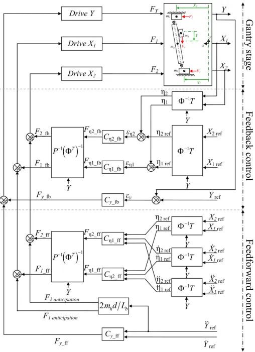
1) A feedforward control structure (bottom of Fig.4), which is obtained by inversion of the decoupling basis model (32). This model inversion is performed using the Energetic Macroscopic Representation (EMR) formalism (Barre, et al., 2006). The feedforward control starts from the reference positions, velocities, and accelerations X1 ref, X2 ref, and Yref. These references are transformed into the equivalent decoupling basis

references η1 ref, η2 ref and Yref, using (39). Each decoupled reference is then fed into its respective controller Cη1_ff, Cη2_ff, and Cy_ff. Finally, the calculated feedforward forces Fη1_ff (40), Fη2_ff (41), and Fy_ff (42) are

transformed into the reference forces F1_ff, F2_ff, and Fy_ff using (43). The compensation of the dynamics of the

payload (24) is added to the reference forces F1_ff and F2_ff.

1 1 12 1 2 2 1 0 1 2 1 2 0 0 1 0 ; 1 1 0 0 0 1 0b 0 b 1 X T X T L L Y Y                               _ _       = (39)

1ref 1_ff 1_ff 1ref 1_ff g1 2 1ref 1 2 0 g b T h m m m F C C c c m       _{ }               _      (40)







 











2 2 2 2 1 2 12 2 ref 2 2_ff 2_ff 2 ref 2_ff g1 g2 12 12 2 re 1 2 1 2 1 2 f 2 4 4 b h b b b b T b h b h b b J J m m L m d Y m m m m F C C c c c L L k c k                              _    _ _          (41) ref _ff _ff ref _ff ref 0 y T h y y y c Y _m F C Y C Y   _{ }   _{ }  _{ }            (42)

 

1 1 ₁ 1 2 2 1 1 0 2 2 0 0 0 1 T b b Y Y F F F P F P L L F F                          _ _     = (43)

2) A feedback control structure (middle of Fig.4). The decoupling basis feedforward control provides most of the dynamic response of the gantry stage (i.e. coarse positioning). In the same way, it compensates for the unbalance and mechanical coupling between actuators. Nevertheless, it does not compensate for non–modeled disturbances, uncertainties on the model parameters and neglected phenomena. Thus, to improve the fine positioning of the gantry stage, a decoupling basis feedback control is proposed. Its structure is similar to those of the feedforward control. It starts from the reference positions X1 ref, X2 ref and Yref, which are transformed into the decoupled

references η1 ref, η2 ref and Yref using (39). These references are then fed into classical industrial PID controllers.

They generate the feedback decoupling basis force references Fη1_fb, Fη2_fb and Fy_fb, which are the transformed

into the reference forces F1_fb, F2_fb and Fy_fb using (43).

3) Implemented control. The reference forces from the feedback and feedforward controls are added and fed into the drives controlling actuators X1, X2 and Y (top of Fig. 4). Finally, to cancel residual vibrations of the support

structure, a jerk time of 26.5 ms is added to the references X1ref and X2ref. This reduces the solicitation of the first

vibration mode (37.7 Hz) of the supporting structure along the X–direction. Along the Y–direction no jerk time is added. This is because, on this direction, the vibrations are of small amplitude and they disappear rapidly.

Fig. 4 Feedback–feedforward decoupled control structure.

To sum up, using the proposed model-based decoupling control scheme, the factors associated with the coupling effect are compensated as follows: the disturbance associated with the acceleration of the payload is compensated by anticipation. The non-uniform load distribution associated with the variable position of the payload, and the coupling due to different motor characteristics is implicitly taken into account by the modal transformation. In the decoupled frame, the translation controller handles the synchronizing motion of actuators

X1 and X2 while the rotation controller rejects un-modeled disturbances affecting their synchronization.

Fη1_ff Fη2_ff m1 m2 mb mh Y x y F2 F1 Fy X2 X1 X1 X2 F1 F2 1_T   Y η2 η1 Y FY Y X2 ref X1 ref X2 ref X1 ref X2 ref X2 ref X1 ref X1 ref Y Y 1_T   Y . . .. .. η2 ref η1 ref Cη2_fb Cη1_fb

 

1 1 T P _  Y Fη2_fb Fη1_fb εη2 εη1 F2_fb F1_fb η2 ref η1 ref η2 ref η1 ref η2 ref η1 ref . . .. .. Cη2_ff Cη1_ff

 

1 1 T P     Y Cy_fb εy Y ref Fy_fb F2_ff F1_ff Cy_ff Fy_ff Y ref .. Y ref .

2

m d L

_{h b} F2 anticipation F1 anticipation Drive Y Drive X1 Drive X2

Gantr

y sta

ge

Feedback control

Feed

for

w

ar

d co

ntr

ol

1_T   1_T   1_T  

4 EXPERIMENTAL VALIDATION

In this section, independent axis control and the proposed decoupling basis control are compared. First, two point–to–point motion examples are presented, then a Ballbar test (path–tracking motion) is proposed.

4.1 Point–to–point motion tests

The first test consists in synchronously displacing X1 and X2 from –0.2 m to +0.2 m at a maximum velocity of

2 m/s and acceleration of 20 m/s². For the first motion example (Fig.5), position references are generated with a 26.5 ms jerk time, the payload is kept immobile at 0.2 m. In this configuration of the Y–axis, the unbalance between X1 and X2 actuators is at its maximum value.

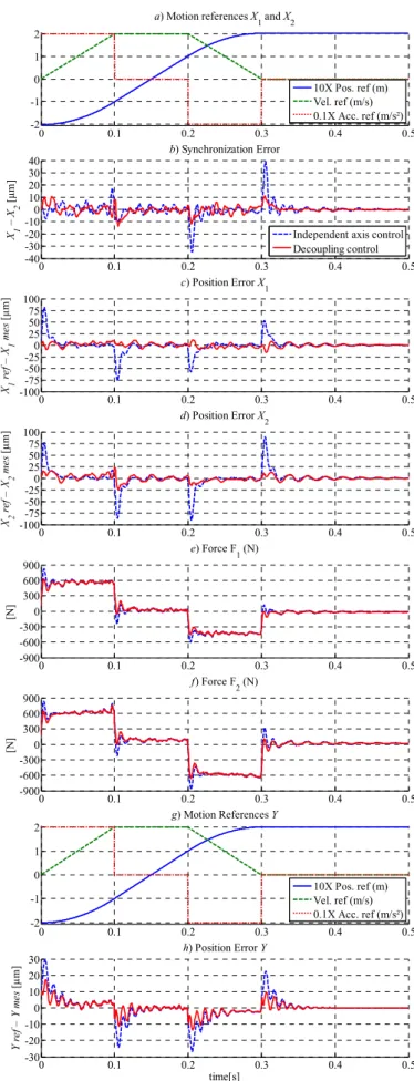
The second test consists in displacing the payload along a diagonal over the machine workspace. Trajectories for axes X1, X2, and Y are identical. They move from –0.2 m to +0.2 m at a maximum velocity of 2 m/s and a

maximum acceleration of 20 m/s². During this motion, the gantry stage goes from an extreme unbalance condition to the other. Due to the acceleration of the payload, the coupling between the Y–axis and actuators X1

and X2 is important. To exacerbate this phenomenon, the jerk time has been set to zero for all axes (Fig.6).

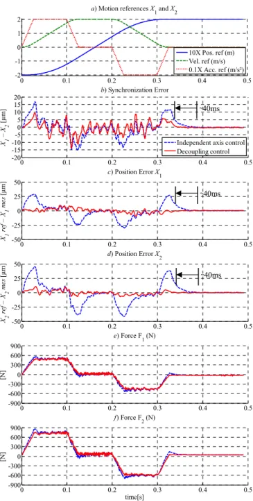
Figs. 5 and 6, allow verifying that controlling the gantry stage on a decoupling basis results in an improvement of the synchronization of actuators X1 and X2 and in a reduction of more than 50% of the position error during

acceleration shifts. Moreover, when jerk time is well tuned (Fig.5), the settling time is significantly reduced, i.e. a reduction of about 10%, compared to the independent axis control. The remaining oscillations on the synchronization and on position tracking errors are mostly due to the detent forces of the PMLSMs.

Another advantage of the decoupling basis approach is a reduction of about 12% of the peak force of actuators

X1 and X2, as shown on force plots in Figs.5 and 6. So, future versions of the gantry stage using the model-based

decoupling control proposed in this paper could be designed with less powerful actuators for X1 and X2. This is

an economical advantage for manufacturers insofar as gantry stages will be more efficient at reduced production costs.

Fig. 5: Independent axis control vs. decoupling basis control, point–to–point X1 and X2 synchronized motions

(from –0.2 to +0.2 m) at a maximum velocity of 2 m/s and a maximum acceleration of 20 m/s²; the position of the payload is kept at 0.2 m (i.e. maximum unbalance).

0 0.1 0.2 0.3 0.4 0.5 -2 -1 0 1 2

a) Motion references X₁ and X₂

10X Pos. ref (m) Vel. ref (m/s) 0.1X Acc. ref (m/s²) 0 0.1 0.2 0.3 0.4 0.5 -20 -15 -10-5 0 5 10 15 20 X1 – X 2 [µ m ] b) Synchronization Error

Independent axis control Decoupling control 0 0.1 0.2 0.3 0.4 0.5 -50 -25 0 25 50 X1 re f – X1 me s [µm ] c) Position Error X₁ 0 0.1 0.2 0.3 0.4 0.5 -50 -25 0 25 50 X2 re f – X2 me s [µm ] d) Position Error X₂ 0 0.1 0.2 0.3 0.4 0.5 -900 -600 -300 0 300 600 900 [N ] e) Force F₁ (N) 0 0.1 0.2 0.3 0.4 0.5 -900 -600 -300 0 300 600 900 time[s] [N ] f) Force F₂(N) ~40ms ~40ms ~40ms 

Fig. 6: Independent axis control vs. decoupling basis control, point–to–point diagonal movement (X1, X2, and Y

from –0.2 to +0.2 m) at a maximum velocity of 2 m/s and a maximum acceleration of 20 m/s².

0 0.1 0.2 0.3 0.4 0.5 -2 -1 0 1 2

a) Motion references X₁ and X₂

10X Pos. ref (m) Vel. ref (m/s) 0.1X Acc. ref (m/s²) 0 0.1 0.2 0.3 0.4 0.5 -40 -30 -20 -100 10 20 30 40 X1 – X 2 [µm ] b) Synchronization Error

Independent axis control Decoupling control 0 0.1 0.2 0.3 0.4 0.5 -100-75 -50 -250 25 50 75 100 X1 re f – X1 me s [µm] c) Position Error X₁ 0 0.1 0.2 0.3 0.4 0.5 -100-75 -50 -250 25 50 75 100 X2 re f – X2 me s [µ m ] d) Position Error X 2 0 0.1 0.2 0.3 0.4 0.5 -900 -600 -300 0 300 600 900 [N ] e) Force F₁(N) 0 0.1 0.2 0.3 0.4 0.5 -900 -600 -300 0 300 600 900 [N ] f) Force F₂ (N) 0 0.1 0.2 0.3 0.4 0.5 -2 -1 0 1 2 g) Motion References Y 10X Pos. ref (m) Vel. ref (m/s) 0.1X Acc. ref (m/s²) 0 0.1 0.2 0.3 0.4 0.5 -30 -20 -10 0 10 20 30 time[s] Y re f – Y me s [µ m ] h) Position Error Y

4.2 Ballbar tests

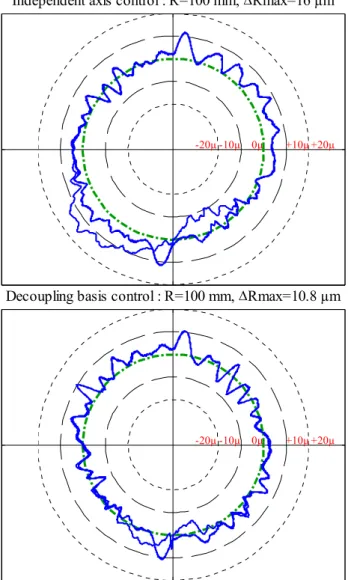
This test consists in tracing clockwise three concentric circles of 100 mm radius. The test results are presented thanks to ballbars, see Fig.7. The dash dot circle represents the reference. The plotted radius error is amplified a million times. The measurement precision is 1µm.

The first circle is traced during the tangential acceleration cycle of the payload; the peak acceleration of actuators

X1, X2, and Y is 16 m/s². At the end of this cycle, the payload has reached a constant tangential velocity of 1.3

m/s. The second circle is traced at this velocity. The third and final circle is traced during the deceleration cycle.

The effect of the mechanical coupling on the tracking precision is easy to identify thanks to a comparison between the two ballbars of Fig. 7. This is specially highlighted during the tangential acceleration and deceleration phases. To take into account the unbalance and the mechanical coupling between actuators within the control structure results in a minimization of 33% of the maximum radius error and in a global minimization of the mean error. This represents a significant improvement in tracking precision performances. The remaining error has a cyclic shape function of the actuators' positions and is mostly due to the detent forces of the PMLSMs. This error can be compensated for example by considering the coordinated motion control of the decoupled motions X and Y, as in (Yang & Li, 2011) and (Hu, Yao, & Wang, 2011), so that the path-tracking performance can be further improved.

Fig. 7: Independent axis control vs. decoupling basis control. Ballbar tests realized with three 100 mm radius circles at a maximum tangential velocity of 1.3 m/s and acceleration of 16 m/s².

5 CONCLUSION

In this paper, a model-based decoupling control method for dual-drive gantry stages is presented. First, a dynamical model of the gantry stage is presented in terms of coordinates (X, Θ, Y). Where, X and Θ define, respectively, the translation and the rotation of the transverse member of the gantry stage, Y defines the translation of the payload. This model accounts for the coupling effects associated with the interaction between the actuators constituting the gantry stage. To make this model adaptable to various types of gantry stages, an identification method (that can be easily implemented using independent axis control) is also presented. The second part of the paper is devoted to the model-based decoupling control of gantry stages. As described, via feedforward compensation, it is possible to fully decouple the dynamics of the payload from the rest of the

0µ

-10µ +10µ

-20µ +20µ

Independent axis control : R=100 mm, Rmax=16 µm

0µ

-10µ +10µ

-20µ +20µ

system. Thanks to this pre-decoupling, the remaining system dynamics (defined now in terms of coordinates X and Θ) can be easily decoupled by interpreting it as an eigenvalue problem. Without this pre-decoupling, the orthogonalization of the motion equations of the gantry stage would have been more laborious and computationally more expensive due to the repeated eigenvalues associated with the rigid motions X and Y. The decoupled model that is obtained using the pre-decoupling approach is also a physical model. It describes the dynamics of the gantry stage in terms of the total mass in translation and in rotation; two motions that are naturally decoupled. Based on this description, a decoupling feedforward/feedback control scheme was derived by model inversion. Experimental results show that in comparison to the industrial independent axis control, the proposed model-based decoupling control lead to a significant improvement of the positioning performance of the gantry stage.

The contribution of this paper is by no means limited to the model-based decoupling control method that is presented here. Indeed, the proposed modeling of the gantry stage, along with the proposed identification method, can be used as a base to develop other control architectures. This will be the subject of future papers.

6 ACKNOLEDGMENT

This research project is funded and supported by ETEL SA. http://www.etel.ch and the CIFRE research grant No. 448/2008 of the French National Association of Research and Technology.

7 REFERENCES

Bagordo, G., Cazzulani, G., Resta, F., & Ripamonti, F. (2011). A modal disturbance estimator for vibration suppresion in nonlinear flexible structures. Journal of Sound and Vibration , 330, 6061-6069.

Barre, P., Bouscayrol, A., Delarue, P., Dumetz, E., Giraud, F., Hautier, J., et al. (2006). Inversion-based control of electromechanical systems using causal graphical descriptions. IEEE-IECON'06 - 32nd Annual Conference on

Industrial Electronics, (pp. 5276-5281).

Chang, Y., Nguyen, T., & Wang, C. (2010). Design and Implementation of look-ahead linear jerk filter for a computerized numerical controller machine. Control Engineering Practice , 18 (12), 1399-1405.

Giam, T., Tan, K., & Huang, S. (2007). Precision coordinated motion of multi-axis gantry stages. ISA

Transactions , 46 (3), 399-409.

Higham, N. (2002). Accuracy and Stability of Numerical Algorithms (2nd ed. ed.). Society for Industrial and Applied Mathematics.

Hu, C., Yao, B., & Wang, Q. (2011). Global Task Coordinate Frame-Based Contouring Control of Linear-Motor-Driven Biaxial Systems With Accurate Parameter Estimations. IEEE Transactions on Industrial

Electronics , 58 (11), 5195-5205.

Hu, C., Yao, B., & Wang, Q. (2010). Integrated direct/indirect adaptative robust contouring control of a biaxial gantry with accurate parameters estimation. Automatica , 46, 701-707.

Lin, F., & Shen, P. (2006). Robust fuzzy neural network sliding-mode control for two axis motion control system. IEEE Transactions on Industrial Electronics , 53 (4), 1209-1225.

Lin, F.-J., Chou, P.-H., Chen, C.-S., & Lin, Y.-S. (2011). DSP-Based Cross-Coupled Synchronous Control for Dual Linear Motors via Intelligent. IEEE Transactions on Industrial Electronics .

Meirovitch, L. (1990). Dynamics and Control of Structures. Wiley Interscience.

Tan, K., Lim, S., Huang, S., Dou, H., & Giam, T. (2004). Coordinated motion control of moving gantry stages for precision applications based on an observer-augmented composite controller. IEEE Transactions on Control

Systems Technology , 12 (6), 984-991.

Teo, C., Tan, K., Lim, S., Huang, S., & Tay, E. (2007). Dynamic modeling and adaptative control of a H-type gantry stage. Mechatronics , 17 (7), 361-367.

Van Dijk, J., Tinsel, R., & Schrijver, E. (2001). Comparison of two iterative learning concepts applied on a manipulator with cogging force disturbances. IFAC Workshop on Adaptation and Learning in Control and

Signal Processing, (pp. 71-76).

Yang, J., & Li, Z. (2011). A Novel Contour Error Estimation for Position Loop-Based Cross-Coupled Control.

IEEE/ASME Transactions on Mechatronics , 16 (4), 643-655.

Yousefi, H., Hirnoven, M., Handroos, H., & Soleymani, A. (2008). Application of neural network in suppressing mechanical vibration of a permanent magnet linear motor. Control Engineering Practice , 16 (7), 787-797.

Figure Legends

Fig. 1 Dual–drive H–type gantry stage provided by ETEL

Fig. 2 Lumped–parameter model of the Dual–drive H–type gantry stage

Fig. 3 Experimental and simulation responses of a) Motion references X1 and X2; b) Synchronization Error;

Position Error of c) X1 axis, d) X2 axis; e) Motion references Y; and f) position error of Y axis. Test realized using

independent axis control for a displacement of – 0.2 m to 0.2 m for all axes, at a maximum speed of 2 m/s, and a maximum acceleration of 20 m/s².

Fig. 4 Feedback–feedforward decoupled control structure.

Fig. 5: Independent axis control vs. decoupling basis control, point–to–point X1 and X2 synchronized motions

(from –0.2 to +0.2 m) at a maximum velocity of 2 m/s and a maximum acceleration of 20 m/s²; the position of the payload is kept at 0.2 m (i.e. maximum unbalance).

Fig. 6: Independent axis control vs. decoupling basis control, point–to–point diagonal movement (X1, X2, and Y

from –0.2 to +0.2 m) at a maximum velocity of 2 m/s and a maximum acceleration of 20 m/s².

Fig. 7: Independent axis control vs. decoupling basis control. Ballbar tests realized with three 100 mm radius circles at a maximum tangential velocity of 1.3 m/s and acceleration of 16 m/s².