ÉCOLE DE TECHNOLOGIE SUPÉRIEURE UNIVERSITÉ DU QUÉBEC
THESIS PRESENTED TO
ÉCOLE DE TECHNOLOGIE SUPÉRIEURE
IN PARTIAL FULFILLMENT OF THE REQUIREMENTS FOR A MASTER’S DEGREE IN ELECTRICAL ENGINEERING
M. Eng.
BY
Thomas DELAPORTE
REAL-TIME KINEMATIC SOFTWARE USING ROBUST KALMAN FILTER AND DUAL-FREQUENCY GPS SIGNALS FOR HIGH PRECISION POSITIONING
MONTRÉAL, SEPTEMBER 4th 2009 © Thomas Delaporte, 2009
BOARD OF EXAMINERS
THIS THESIS HAS BEEN EVALUATED BY THE FOLLOWING BOARD OF EXAMINERS
Dr René Jr. Landry, thesis supervisor
Department of electrical engineering at the École de technologie supérieure
Dr Nicolas Constantin, president of the board of examiners
Department of electrical engineering at the École de technologie supérieure
Dr Mohamed Sahmoudi, examiner
Department of electrical engineering at the École de technologie supérieure
Dr Rock Santerre, examiner
Departement of geomatics sciences at Université Laval, Québec
Dr Peter Nuytkens, examiner Q Developments LLC, Boston
THIS THESIS HAS BEEN PRESENTED AND DEFENDED BEFORE A BOARD OF EXAMINERS AND PUBLIC
AUGUST 27th 2009
ACKNOWLEDGEMENTS
I would like to thank my professor Dr. René Jr. Landry for the opportunity he gave me to study the field of Global Navigation Satellite System (GNSS) technology.
I would like also to thank my friends and colleagues Jean-Christophe Guay and Guillaume Lamontagne for being around during my master thesis in Quebec. Also, I would like to thank Marc-Antoine Fortin, Dr. Di Li, Philipe Lavoie, Bruno Sauriol and Nick Lui for their supports and companionship.
Special thank to Fauve for supporting me during those two years, and my parents, brothers and little sister.
To conclude, I would like also to thank our partner Gedex and the NSERC, without whom this project would not have been possible.
REAL-TIME KINEMATIC SOFTWARE USING ROBUST KALMAN FILTER AND DUAL-FREQUENCY GPS SIGNALS FOR HIGH PRECISION POSITIONING
Thomas DELAPORTE ABSTRACT
The Global positioning System (GPS) started in the 1970’s with an ambitious project of U.S positioning service using satellites. It has now become one of the major technologies for positioning people and objects around the planet, with diverse application in mapping and localization. GPS has overcome all its expectation, providing signal continuously around the entire planet, providing positioning service more and more precise. Future constellation will now arise, like GALILEO for Europe or COMPASS for China, bringing more attractive, precise and powerful applications. The modernization programs of GPS and Russian GLONASS will brings even more capabilities for worldwide users.
One of the most interesting applications of GPS is the Real-Time Kinematic system. This technique emerged in the beginning of the 1990’s offers centimeter to millimeter precision to the GPS users, using carrier phase measurements and a reference GPS station. It uses differential corrections, and techniques of carrier phase ambiguity resolution ‘on the fly’. It has been successfully applied in geophysics and survey. Unfortunately, such RTK system is only precise in short range from the base station, that is to say less than about 20 km. When the distance from the base station increases, systematic errors are decorrelated. These errors reduce the ambiguity resolution success rate and decrease position precision and reliability. The purpose of this thesis is to overcome these limitations to bring full RTK precision and reliability for long baseline scenarios, up to 80 km.
To fulfill this purpose, a new concept of RTK system for real-time has been developed. This means the development of complete real-time GPS positioning software providing centimeter precision in a robust way for short and long baseline scenario. Different issues have been developed, such as real-time satellite management, robust Kalman filter implementation, and reliable ambiguity resolution technique. The long baseline problem has been developed and overcome using real-time atmospheric modeling and control of the geometric errors. This work presents the different new concepts used in the algorithm and the innovative technique for future system and developments using RTK positioning
To demonstrate the reliability and the performance of the developed algorithm, data from Novatel and NRG-GNSS receiver have been intensively analyzed and processed. With static and dynamic short baseline real-time data, this new developed RTK software presents robust real-time centimeter to millimeter solution precision and fast and reliable ambiguity resolution. Results from the solution are analyzed and the parameters of the real-time
solution are discussed. After validating these scenarios, long baseline dynamic data, coming from our industrial partner Gedex, have been processed in real-time mode. The solution uses the innovative concepts of ionospheric modeling in real-time, and the results present millimeter difference to the post-process Waypoint software. Impact of real-time management and ambiguity resolution technique are presented. The efficiency and precision of the solution opens the RTK solution to new purposes for research and development.
Keyword: GPS, GNSS, RTK, real-time, ambiguity, carrier-phase, robustness, long baseline, Kalman filter.
LOGICIEL TEMPS RÉEL UTILISANT UN FILTRE DE KALMAN ROBUSTE ET DES SIGNAUX GPS DOUBLE FREQUENCES POUR UN POSITIONNEMENT
DE HAUTE PRÉCISION
Thomas DELAPORTE RÉSUMÉ
Le système GPS est une technologie qui a transformée la notion de positionnement pour l’homme par rapport à la terre. Depuis sa mise en route dans les années 1970s, il s’est imposé dans toutes les applications de localisation, avec des systèmes de plus en plus précis, pour le commercial et la recherche, de la cartographie au militaire, en passant par l’aide à la navigation. Le système a dépassé toutes les attentes pour les utilisateurs. L’arrivée de nouvelles constellations, à l’instar de GALILEO pour l’Europe ou de COMPASS pour la Chine, et même la modernisation du GPS et du système Russe GLONASS, créera de nouveaux besoins innovants, en augmentant la précision, la couverture et la disponibilité.
Une des applications les plus intéressantes du GPS est le Real Time Kinematic (RTK). Cette technique apparue dans les années 1990 permet un positionnement d’une précision centimétrique pour les utilisateurs civils. Cette incroyable précision vient tout d’abord de l’utilisation d’une station de base, qui transmet des corrections différentielles pour les signaux GPS. Ensuite, l’utilisation de la phase des signaux et les techniques de résolution d’ambiguïtés en temps réel ont permis d’atteindre une telle précision. Cette technique est aujourd’hui beaucoup utilisée pour la géodésie et par les arpenteurs pour déterminer de façon très précise les courbures de la terre et les nivellements. Mais cette technique possède des limitations, notamment lorsque la distance entre la base et l’utilisateur dépasse 20 km. Dans ces cas de long distance, les erreurs liées à la base et à l’utilisateur ne sont plus identiques. Ces erreurs dégradent les performances de résolutions d’ambiguïtés et la précision de la solution. Le but de ce mémoire est de présenter des solutions innovantes pour apporter toute la précision du RTK dans les cas de longues distances.
Pour parvenir à ce but, une nouvelle approche d’un système RTK fonctionnant en temps réel a été développée. C'est-à-dire un système de positionnement de niveau centimétrique complet utilisable en temps réel par des récepteurs GPS sur de longues distances. L’implémentation d’un tel système prend tout d’abord en compte la gestion temps réel des données et des satellites, une estimation robuste de la position à travers un filtre de Kalman et une technologie améliorée de résolution des ambigüités de phase. Ensuite, le problème de longues distances est abordé et de nouvelles solutions ont été apportées pour résoudre les problèmes liés à cette configuration. Une approche innovante en temps réel a été développée pour les corrections atmosphériques, notamment l’ionosphère, ainsi qu’un contrôle des erreurs géométriques. Cette thèse présente des concepts et des solutions innovantes qui
pourront également servir à de nouvelles applications lors de l’apparition des nouvelles fréquences et constellations.
Pour valider le système et démontrer les capacités innovantes de l’algorithme développé, des données temps réel provenant de récepteurs Novatel, ainsi que du nouveau récepteur universel du LACIME-GRN ont été utilisées. Avec des scenarios en courte distance, statiques et dynamiques, le nouveau système RTK présente une solution robuste de précision centimétrique, avec une résolution d’ambigüités rapide et fiable. Des données longue distance provenant de notre partenaire industriel Gedex sont également analysées. La solution utilisant l’algorithme robuste RTK ainsi qu’une modélisation des erreurs ionosphériques en temps réel présente des résultats identiques au millimètre près comparé au logiciel de traitement Waypoint. Cette validation des performances emmène la technologie RTK présentée vers de nouvelles perspectives pour la recherche et l’industrie.
Mots clés: GPS, GNSS, RTK, temps réel, ambiguïtés, phase, robustesse, filtre de Kalman, longue distance.
TABLE OF CONTENTS
Page
INTRODUCTION ... 22
CHAPTER 1 HISTORY AND PERSPECTIVE OF GNSS FOR PRECISE POSITIONING ...25
1.1 Overview of GNSS history ... 25
1.2 Evolution of the GNSS and the satellite constellations ... 26
1.2.1 GPS Space Segment: from Block II to Block IIF ...26
1.2.2 Other satellite constellations ...27
1.2.3 SBAS system, a novel constellation ...28
1.3 Signals for high precision positioning ... 30
1.3.1 Actual GNSS signals...30
1.3.2 New GNSS Signals ...31
1.4 From DGPS to network RTK ... 32
1.4.1 Differential Global Positioning System ...32
1.4.2 Development of RTK technology ...33
1.4.3 Future evolution of RTK ...34
CHAPTER 2 OBSERVATIONS FROM THE GPS SIGNALS AND THEIR ASSOCIATED ERRORS FOR PRECISE POSITIONING ...37
2.1 Backgrounds ... 37
2.2 Pseudo-range and carrier phase observations overview ... 38
2.2.1 Pseudo-range measurement ...38
2.2.2 Carrier phase measurements ...40
2.2.3 Doppler measurements...43
2.2.4 Summary of the GPS observations ...44
2.3 Details of common errors for all the observations ... 46
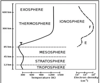
2.3.1 Troposphere delays ...46
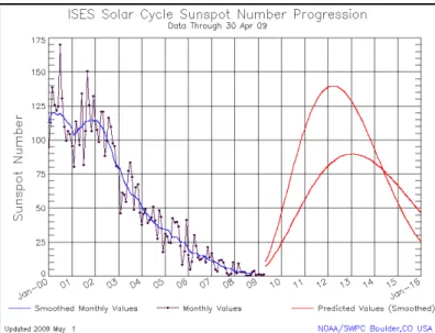
2.3.2 Ionosphere delays...48
2.3.3 Satellite ephemerides errors and its impact on positioning ...52
2.3.4 Other common-mode error ...53
2.4 Details of non-common errors for all observations ... 53
2.4.1 Multipath error ...53
2.4.2 Receiver noise ...54
2.5 Expression of double difference measurements ... 55
CHAPTER 3 ROBUST KALMAN FILTER FOR REAL-TIME HIGH PRECISION POSITION ESTIMATION ...59
3.1 Satellite management in the Kalman filter ... 60
3.1.1 Satellite selection criterions ...60
3.1.2 Stochastic model assignment of the satellite receiver measurements ...61
3.2.1 State vector, the functional model and associated variance ...65
3.2.2 Observation model ...68
3.2.3 Recursive equations of the Kalman filter ...71
3.2.4 Robust management of the observations ...73
3.3 Ambiguity resolution of the carrier phase ... 75
3.3.1 Using the dual-frequency ADR to combine ambiguities ...75
3.3.2 Overview of the resolution of the double difference ambiguity ...76
3.3.3 Overview of the LAMBDA method ...77
3.3.4 Validation method for the fixed ambiguities ...82
3.4 Global summary of the complete RTK technique ... 84
CHAPTER 4 ALGORITHM VALIDATION FOR SHORT BASELINE RTK USING LACIME-NRG GNSS AND NOVATEL RECEIVERS ...86
4.1 Introduction ... 86
4.2 Static analysis and performance of the GNSS receiver ... 87
4.2.1 Static double difference measurements precision ...87
4.2.2 Float Solution results for GNSS and Novatel configuration ...91
4.2.3 Ambiguity resolution results and fixed solution analysis ...95
4.3 Analysis of the kinematic mode with both Novatel receivers (short baseline) ... 100
4.3.1 Experimental procedure ...100
4.3.2 Float and fixed solution results ...101
4.3.3 Velocity error of the dynamic solution ...105
4.3.4 Ambiguity resolution ...107
CHAPTER 5 CORRECTIONS FOR MEDIUM AND LONG BASELINE RTK AND RESULTS ...109
5.1 Presentation of the ionosphere modeling estimation for medium and long baseline scenario ... 110
5.1.1 Ionosphere error state in the weighted ionosphere estimation. ...111
5.1.2 Ionosphere pseudo-observations in the weighted ionosphere model ...114
5.1.3 Other non-common errors corrections ...116
5.2 Static validation of the ionosphere weighting scheme for medium baseline ... 118
5.2.1 Experimental procedure and methodology ...118
5.2.2 Ionosphere estimation of the medium baseline solution ...119
5.2.3 Solution precision using two different ionospheric corrections ...121
5.2.4 Ambiguity resolution performance ...123
5.3 Analysis of long baseline high dynamic test ... 125
5.3.1 Experimental procedure ...125
5.3.2 Atmospheric errors estimation using the ionosphere weighted model ...127
5.3.3 Ambiguity resolution performance of the solution ...130
5.3.4 Analysis of the long baseline fixed solution ...131
CHAPTER 6 CONCLUSION AND RECOMMENDATIONS ...135
6.1 General Conclusion ... 135
ANNEXE I ORBIT/CLOCK SATELLITE DETERMINATION USING
BROADCAST EPHEMERIS ... 139 ANNEXE II RESULTS OF ANOTHER GEDEX FLIGHT, FOR MEDIUM
BASELINE HIGH DYNAMIC SCENARIOS ... 144 ANNEXE III OVERVIEW OF THE RTK SOFTWARE AND THE C FUNCTIONS
FOR RTK POSITIONING USING NOVATEL AND GNSS
RECEIVER. ... 148 REFERENCES ... 151
LIST OF TABLES
Page
Table 1.1 Evolution and characteristics of the GPS Blocks ...27
Table 2.1 Summary of the main GPS observations with associated errors ...44
Table 2.2 Summary of GNSS signal measurement errors ...45
Table 2.3 Errors related to atmospheric delays in absolute mode ...51
Table 2.4 Approximate relation between ephemerides errors dr and baseline error db from (Leick 2003) ...52
Table 2.5 Receiver noise for code and phase measurements...55
Table 4.1 Standard deviation of Pseudo-range and carrier phase measurement for GNSS and Novatel Double difference, and related medium elevation angle ...90
Table 4.2 General User Range Error analysis of GPS measurements in short baseline ...91
Table 4.3 Standard deviation (std) of the FLOAT solution for the two configurations: the Novatel configuration and the GNSS configuration using known position. ...95
Table 4.4 Standard deviation of the fixed solution errors for the Novatel and the GNSS configurations, and the difference between the two configurations solution. ...98
Table 4.5 Ambiguity success rate and Time to First Fix ...99
Table 4.6 Standard deviation of the solution for the LLH axes ...104
Table 4.7 Standard deviation of the velocity solution for the two modes ...107
Table 4.8 Ambiguity success rate and Time to First Fix for dynamic short baseline test ...108
Table 5.1 Ionosphere standard deviation (1σ) for the iono-weighted and iono-free solution for each DD satellite and the associated satellite elevation angle ...120
Table 5.2 Standard deviation of the iono-free and iono-weighted solution for the geographic axes compared to the mean Waypoint solution ...122
Table 5.3 Ambiguity success rate and Time to First Fix using iono-free
modeling ...124 Table 5.4 Standard deviation of the DD ionospheric errors during process ...128 Table 5.5 Ambiguity success rate and Time to First Fix (TFF) using Ionospheric
modeling ...130 Table 5.6 Standard deviation of the RTK solution for the long baseline test
(maximum of 140 km), compared to the post-process Waypoint
LIST OF FIGURES
Page
Figure 1.1 Principle of DGPS for marine coast guard. ...32
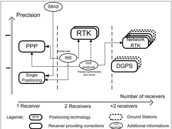
Figure 1.2 Summary of the different positioning technology in terms of precision and number of receivers. ...35
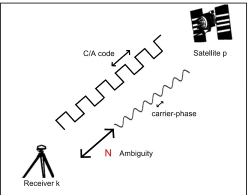
Figure 2.1 Representation of the carrier-phase measurement’s ambiguity. ...40
Figure 2.2 Atmospheric layers of the earth. ...46
Figure 2.3 Predicted solar activities. from (noaanews.noaa.gov) ...49
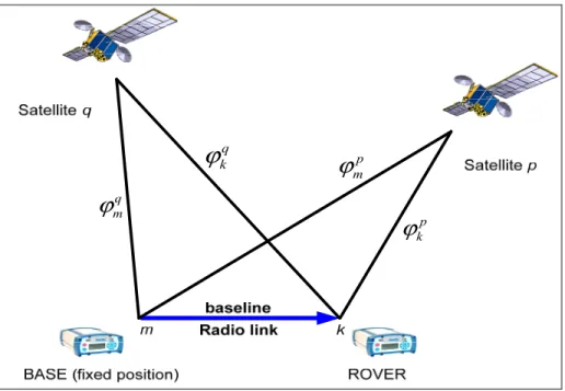
Figure 2.4 Method of double difference between two receivers k and m and two satellites p and q for the ADR measurements. ...55
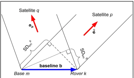
Figure 3.1 Geometrical view of the double difference measurement in the observation model. ...69
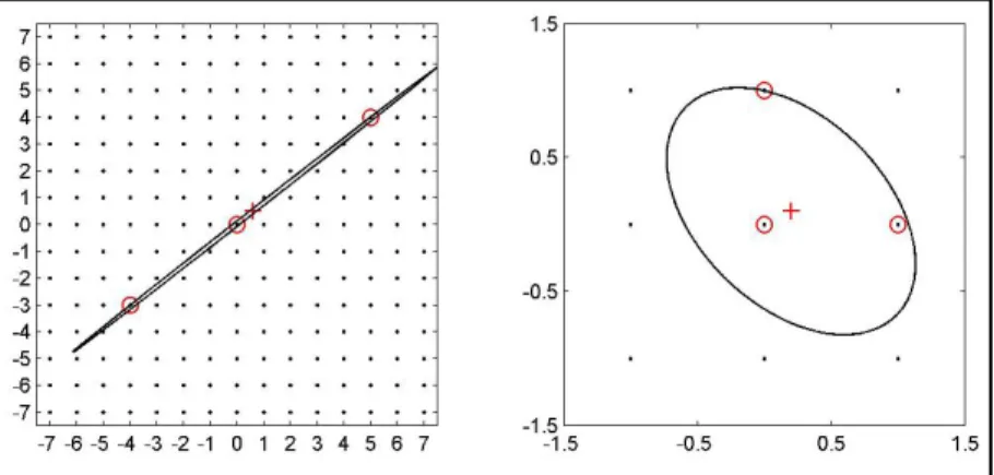
Figure 3.2 Transformation of the ellipsoid search space using Z-transformation. ...80
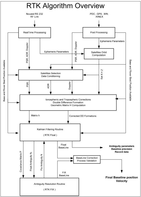
Figure 3.3 Overview of the global Kalman filter procedure for the RTK algorithm. ...85
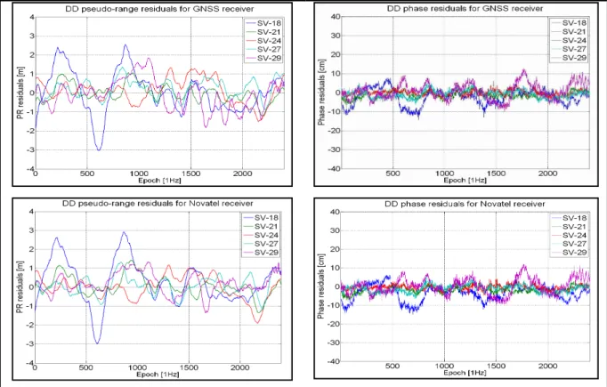
Figure 4.1 Analysis of measurements double difference residuals for the GNSS-Novatel and GNSS-Novatel-GNSS-Novatel pair of rover-base in static mode, using known baseline position. ...89
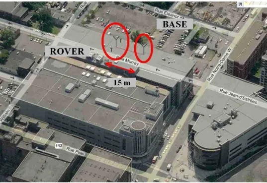
Figure 4.2 Static configuration of the antennas on the ETS rooftop. ...92
Figure 4.3 Geographic error of the position using the RTK software in float mode with the Novatel configuration for short baseline static test at ETS. ...93
Figure 4.4 Geographic error of the position using the RTK software in float mode with the GNSS configuration for short baseline static test at ETS. ...93
Figure 4.5 Number of GPS satellites used in the RTK solution and the associated PDOP for the Novatel and GNSS configuration. ...94
Figure 4.6 Geographic error of the position using the RTK software in fixed mode with the Novatel configuration for short baseline static test at ETS. ...96
Figure 4.7 Geographic error of the position using the RTK software in fixed mode with the GNSS configuration for short baseline static test at ETS. ...96
Figure 4.8 Zoom of the geographic error of the position in fixed mode with
Novatel configuration for short baseline test at ETS. ...97
Figure 4.9 Zoom of the geographic error of the position in fixed mode with GNSS configuration for short baseline test at ETS. ...97
Figure 4.10 Solution difference between the Novatel and the GNSS configuration using the same RTK algorithm for the static test at ETS. ...99
Figure 4.11 Installation set-up for the kinematic test recording (cars and receivers). ..100
Figure 4.12 Trajectory of the dynamic test. ...101
Figure 4.13 Number of satellites used in the RTK solution for the kinematic test. ...101
Figure 4.14 Evolution of Position DOP in the RTK solution for the kinematic test. ..101
Figure 4.15 Position error for the float solution in the dynamic test, using Novatel configuration, compared to the Waypoint solution. ...103
Figure 4.16 Position error for the fixed solution error in dynamic test, using Novatel configuration compared to the Waypoint solution...103
Figure 4.17 Evolution of the standard deviation of the position errors for the float solution in dynamic test. ...104
Figure 4.18 Evolution of the standard deviation of the position errors for the fixed solution in dynamic test. ...104
Figure 4.19 Waypoint estimated standard deviation of the position error for the dynamic test. ...105
Figure 4.20 Velocity of the Novatel receiver mounted on the car during the dynamic test. ...106
Figure 4.21 Errors of the rover velocity using the float solution in dynamic compared to Waypoint. ...106
Figure 4.22 Errors of the rover velocity using the fixed solution in dynamic compared to Waypoint. ...106
Figure 4.23 Ambiguity resolution success rate during dynamic test. ...107
Figure 4.24 Evolution of the ratio test during dynamic test...107
Figure 5.1 Static rover antenna installation for the medium baseline test. ...118
Figure 5.3 Number of satellites in use during medium baseline test. ...119
Figure 5.4 Evolution of Position DOP during medium baseline test. ...119
Figure 5.5 DD ionospheric error estimation using iono-free solution. ...120
Figure 5.6 DD ionospheric error estimation using iono-weighted solution. ...120
Figure 5.7 Position precision using iono-free method in the medium baseline test compared to Waypoint ...122
Figure 5.8 Position precision using iono-weighted method in the medium baseline test compared to Waypoint. ...122
Figure 5.9 LAMBDA ratio test using the iono-free method in the medium baseline test. ...124
Figure 5.10 LAMBDA ratio test using the weighted ionosphere method in the medium baseline test. ...124
Figure 5.11 Initial position and starting point of the airplane. ...125
Figure 5.12 Trajectory of the airplane during long baseline test. ...125
Figure 5.13 Trajectory of the airplane in geographic axes. ...126
Figure 5.14 Altitude profil of the airplane during flight. ...126
Figure 5.15 Evolution of the baseline distance during the long baseline test. ...126
Figure 5.16 3D velocity of the airplane during long baseline test. ...126
Figure 5.17 Number of satellites used during long baseline test. ...127
Figure 5.18 Evolution of the Position DOP during long baseline test. ...127
Figure 5.19 Double difference troposheric errors modeling for the long baseline test using Saastamoinen model. ...127
Figure 5.20 Double difference ionospheric errors using the ionosphere-free model for different SV combination. ...129
Figure 5.21 Double difference ionospheric errors using the ionosphere-weighted model for different SV combination. ...129
Figure 5.22 Ambiguity resolution success during the long baseline test. ...130
Figure 5.24 Difference between the geographic RTK solution compared to the
Waypoint solution for the long baseline dynamic test. ...132 Figure 5.25 Zoom on the latitude and longitude axes of the difference between the
RTK solution and the Waypoint solution for the long baseline dynamic test. ...132 Figure 5.26 Evolution of the standard deviation 3D error for the long baseline
solution, compared to Waypoint. ...134 Figure 5.27 Waypoint estimated standard deviation of the 3D position errors. ...134
LIST OF SYMBOLS p
Refers to satellite p k
Refers to receiver k 1 L
Refers to L1 frequency 2 L
Refers to L2 frequency IF
Refers to the iono-free measurementˆ
Refers as fixed values in the LAMBDA method
Refers as ‘true’ values in the LAMBDA methodϕ
Carrier phase observation [radians]P Pseudo-range measurement [m] P• Doppler-range measurement [m/s] dt Clock error bias [m].
dt• Clock error drift [m/s]
ρ
‘True’ range between satellite and receiver [m]ρ
• ‘True’ Doppler range between satellite and receiver [m/s]I Ionospheric delay [m]
T Tropospheric delay [m]
I• Tropospheric delay drift [m/s] T• Ionospheric delay drift [m/s]
c
Speed of light in vacuum [m/s]τ
Time of transmission through spacea Ambiguity parameters in the LAMBDA method b Position vector in the LAMBDA method
x Receiver acceleration
uk Receiver acceleration associated noise f Process function in the system
F Process matrix in the Kalman filter
Q Process covariance matrix in the Kalman filter R Measurements covariance matrix in the Kalman filter X State space vector in the Kalman filter
LIST OF ACRONYMS
ADR Accumulated Doppler Range
BIE Best Integer Equivariant
BOC Binary Offset Code
C/A Coarse Acquisition
DD Double Difference
DGPS Differential GPS
DLL Delay Lock Loop
DOT Department Of Transport
EGNOS European Geostationary Navigation Overlay Service ESA European Space Agency
EU European Union
FAA Federal Aviation Administration FLL Frequency Lock Loop
GAGAN Global And Geo Augmentation System GBAS Ground Based Augmentation System GLONASS GLObal NAvigation System
GNSS Global Navigation Satellite System GPS Global Positioning System
GUI Graphic User Interface
IA Integer Aperture
IB Integer Bootstrapping
IGS International GNSS Service
ILS Instrument Landing System
ILS Integer Least Squares INS Inertial Navigation System
ITRF International Terrestrial Reference Frame LAAS Local Area Augmentation System
LAMBDA Least-squares AMBiguity Decorrelation Adjustments
LT Lock Time
MBOC Multiple Binary Offset Code
MSAS Mult-functional Satellite Augmentation System PCF Probability of Correct Fix
PDOP Position Dilution of Precision
PLL Phase Lock Loop
PPP Precise Point Positioning
PRN Pseudo-Random Noise
PVT Position Velocity Time QZSS Quasi-Zenith satellite System
RTK Real Time Kinematics
SA Selective Availability
SBAS Satellite Based Augmentation System
SD Single Difference
SV Space Vehicle
TEC Total Electron Content
LISTE OF MEASURE UNITS GEOMETRIC UNITS Length km m dm cm mm kilometer meter decimeter centimeter millimeter Angle rad º ’ ” radians degree minute arc second arc MECHANIC UNITS Speed m/s km/h rad/s
meter per second kilometer per hour radian per second Acceleration
m/s2 rad/s2
meter per second square radian per second square Jerk
m/s3
rad/s3 meter per second cube radian per second cube
TIME UNITS h min s ms µs ns ps hour minute second millisecond microsecond nanosecond picosecond FREQUENCY UNITS Hz GHz MHz hertz gigahertz megahertz THERMAL UNITS °C K Celsius degree Kelvin degree ATMOSPHERIC UNITS Pa Pascal pressure
INTRODUCTION
The Global Positioning System (GPS) has transformed the world around us. Today, everyone is able to locate himself precisely on Earth. It has changed the human relation toward space and travels. But this system is also used for the planet itself. With GPS, surveyors and geophysics analyze data to determine the exact geodesy of the planet. It can also monitor small changes in sea level or tectonic movement. How is it possible to achieve such precision and interesting capabilities with this satellite system?
The precision of the GPS improved constantly. When the GPS was launched, the SA (Selective Availability) system intentionally induced noise in the GPS satellite clock, to degrade the position solution. The position solution for civilian was precise at around 100 meters. In May 2000, SA was turned off and the system suddenly becomes more precise, around 5 to 10 meters for civilian users. SA could be overcome because differential positioning technique appeared and this technique is able to remove SA by using differential corrections from a base station. This major technique brings new solution in high precision positioning, such as Real Time Kinematic (RTK).
The basis of RTK technique is to use differential correction from a base station to improve the solution precision. It also uses at the same time the carrier-phase of the signal instead of the common code-phase, for satellite to receiver range determination. In fact, the phase is up to one hundred times more precise than the code itself, allowing a corresponding precision in the solution. The main drawback of using the carrier-phase in RTK is the necessity of an ambiguity resolution technique. Indeed, the carrier phase keeps track of the satellite receiver distance changes at the beginning of each satellite locking, but does not know the initial ambiguity distance. This unknown is called the ambiguity and is an integer cycle in differential technique. The development of RTK has been possible using new integer ambiguity resolution ‘on the fly’. It started with the work of Hwang (Hwang 1991) and has been since then intensively developed for commercial receiver (Neumann, Manz et al. 1996) or real-time industrial system (Kim and Langley 2003).
But the technique still has problems to overcome in order to become a widespread used technique. First, ambiguity resolution and validation is still a major issue, both for solution precision, and also for solution integrity (Teunissen and Verhagen 2007). But the main problem facing the industry is the development of long baseline, when the distance between the base and the rover (i.e. the mobile using the GPS receiver) increased to 100 km and more (Kim and Langley 2000). At this point, the main errors decorrelate and are not completely removed in differential technique, as it is in short baseline (less than 20 km) and in medium baseline (from 20 to 80 km). Atmospheric delays, ephemeris error, degrade the ambiguity resolution success and the solution precision.
The purpose of this work is to overcome these limitations and bring the full RTK precision to real-time long baseline positioning. Our industrial partner, Gedex inc, based in Toronto, need real-time high precision positioning for an aircraft doing mineral survey across Canada with INS material. To achieve this goal, different works have been done in the GRN (Navigation Research Group) at LACIME. First, a state-of-the art real-time RTK algorithm has been developed, mainly working in static and dynamic short baseline scenario, using real-time data from Novatel receiver and the developed LACIME-NRG universal GNSS receiver. Then, the goal was to analyze the specific errors in long baseline, and to find innovative solutions for the new RTK software.
This thesis will start with the history of GPS satellite constellations and signals. It will bring an interesting perspective of the GPS development and the benefit of new coming constellations and new signal frequencies. History of precise positioning is presented as well as the actual and upcoming related technologies. In the second chapter, the observations from the GPS system, namely the pseudo-range, the carrier phase and the Doppler, which are needed to perform a position, are detailed intensively. The errors and parameters related to these signal measurements are analyzed and studies will be presented to correctly define them. The differential technique used in RTK which remove these errors in short baseline is presented with special care.
The chapters three presents the real-time Kalman filter theory developed for the RTK algorithm, from the basics to the state-of-the-art details of such applications. The Kalman filter is presented such a way that other new GNSS signals can be easily inserted in the developed solution to improved global future performance. Functional and stochastic model of the Kalman filter, an important point for reliable and robust estimation are presented in detail. The real-time aspect of this section is highlighted, presenting the different challenge for a robust solution in real-time, as satellite selection and robust ambiguity resolution.
The last two chapters are dedicated to data analysis and performance results. First, the chapter four presents short baseline scenario in static and dynamic mode. Short baseline static tests are used to validate the basics of the developed real-time RTK algorithm. The LACIME-NRG universal GNSS receiver is used and its performances are compared to the Novatel receiver using the algorithm, showing promising results for further research on new signals tracking and positioning technique. Other short baseline test are analyzed, both in static and dynamic mode. The solution precision is at the centimeter level.
In the chapter five, the long baseline problem is finally presented and developed. A real-time ionosphere errors modeling is presented in details, as well as geometric error corrections. Medium static baseline test are analyzed. These tests show faster ambiguity results than classic technique and centimeter precisions. Finally, the long baseline data coming from Gedex are processed with the developed RTK algorithm. The solution shows centimeter precision and has millimeter similarity to the commercial post process Novatel software called Waypoint. This is very promising for further applications and research in the field of high precision RTK positioning.
The conclusion will end this thesis and will summarize the works done during this master degree, the obtained results and the contributions of the Author. Finally, a list of recommendations for further works will be presented in details to orient future research on that field in the NRG laboratory.
CHAPITRE 1
HISTORY AND PERSPECTIVE OF GNSS FOR PRECISE POSITIONING
1.1 Overview of GNSS history
In this section, a brief overview of the Global Navigation Satellite Systems (GNSS) is presented and how it is related to the high precision positioning capabilities offered to the users, both actually and in the future. The GNSS are mainly composed nowadays of the U.S Global Positioning System (GPS) and the Russian GLObal NAvigation Satellite System (GLONASS), but the European Union (EU) has already 2 satellites in orbit with his GALILEO system and China has satellites in orbit with his COMPASS system (also known as Beidou-2) The number of signals available for the users is also increasing, allowing more and more possibilities with new signal processing techniques.
All these systems will provide worldwide positioning capabilities to users. Many others systems (commercial or not) can improve the overall accuracy. One of the most known systems is WAAS (Wide Area Augmentation System), which is a Satellite Base Augmented System (SBAS). But there exist others SBAS like EGNOS (European Geostationary Navigation Overlay Service) or StarFire (Sahmoudi, Landry et al. 2007), and many Ground Based Augmentation System (GBAS) such as Differential GPS (DGPS), which provide corrections and drastically improve the precision for all users, from military to Safety-of-Life operations. Finally, the Real Time Kinematics (RTK) is one of the most precise systems, allowing performance accuracy at the centimeter level.
New techniques have been developed in the past few years to achieve the precision of such systems using only one receiver. The PPP (Precise Point Positioning) system is one of them. It uses undifferenced measurements and, as for RTK, an ambiguity resolution technique. In the same way, network RTK allows users to only one GPS receiver using multiple base corrections.
1.2 Evolution of the GNSS and the satellite constellations
1.2.1 GPS Space Segment: from Block II to Block IIF
The GPS has started with NAVSTAR and the first satellite was launched in 1978 by the U.S Air Force. The GPS constellation is now composed from different generation of satellites: the II/IIA block, the IIR/IIR-M block and the IIF block which is actually in deployment.
The 9 satellites of Block II Satellite Vehicle (SV) were launched from February 1989 through October 1990. None of them is actually in use. The 19 Block IIAs satellites were launched from November 1990 through November 1997. Actually 6 of them are out of use. Despite a design life of 7.5 years, the first constellation of GPS satellite shows an incredible robustness. The satellite Pseudo-Random Noise (PRN) 01 launched on November 1992 was only decommissioned on March 2008, after 16 years of active service! The Block II was implemented with SA capabilities (GlobalSecurity 2007).
The next generation of satellite, the IIR and IIR-M Block, manufactured by Lockheed Martin, were designed to have 33% lower cost and more autonomous capacities. The IIR-M capabilities include developmental military-use-only M-code on the L1 and L2 signals and a civil code on the L2 signal (namely L2C). For block IIR, 12 satellites were successfully launched from July 1997 to November 2004. The first IIR-M Block satellite was launched on September 2005 and 6 are actually in orbit. This makes a total of 32 active GPS satellites in use for general users nowadays.
The GPS IIF satellites will have all of the capabilities of the previous blocks, but will feature an extended design life of 12 years, faster processors with more memory, and a third civil signal, L5. The first launch is planned for 2010. A total of 12 block IIF GPS satellites constellation is planned.
Table 1.1
Evolution and characteristics of the GPS Blocks
Block II Block IIA Block IIR Block IIR-M Block IIF Block III First
launch 1989 1990 1997 2005 2010 ~2014
# of SV 9 19 13 6 12 /
# in Use 0 13 12 6 0 /
Planned completed completed completed 9 12 8
Signals L1 (C/A), L1/L2-P L1 (C/A), L1/L2-P L1 (C/A), L1/L2-P +L1M/L2M, +L2C +L5 +L5
1.2.2 Other satellite constellations
The Russian system named GLONASS, began service in 1983 and was already an operating system like GPS in 1995. The GLONASS constellation consisted of 24 satellites. The lifetime of the satellite constellation was short and the economical and political situation in Russia made the system declined and lost credibility. Today, this system is pursuing successfully and GLONASS commercial receivers, like Javad receivers, can propose higher precision than GPS-only. Twenty-one GLONASS satellites are operating nowadays. The system is intended to be further developed for worldwide users. In a same time, the Russian government allowed more and more resources to the Federal Space Agency for maintenance and development of the system (RussianSpaceAgency 2007).
The Galileo system is a project under development and is proposed to be a 30 satellites navigation system operating by 2013. It is conducted by the EU and the European Space Agency (ESA), to produce a completely autonomous satellite constellation. But the public-private partnership and political situation delayed and drastically changed the program. Today, the Galileo program is financed by the European Community and ESA acts as its procurement and design agent. The 2 Galileo satellites in orbit for now, namely GIOVE-A in December 2005 and GIOVE-B in April 2008, allows the EU to keep the allocated frequencies (Gibbons 2008).
China also has a navigation satellite system under development. The Beidu-2 or COMPASS system will be a constellation of 35 satellites, with 5 geostationary orbit satellites and 30 medium earth orbit satellites which will offer complete coverage of the globe (Gibbons 2008). Compass-M1 is the first experimental satellite launched by China for signal testing, validation and for the frequency filing on April 13th 2007.
One another new coming satellite system to be mentioned is the one by Japan, the Quasi-Zenith Satellite System (QZSS) that will supplement and be interoperable with GPS.
All these system developments show the economic and strategic importance of satellite navigation in nowadays commercial applications and economy. Taking GPS as a model and trying to improve it, the new satellite constellations will be a great benefit for users. There will be more satellite coverage, more interoperate signals, more robustness and this will improve accessibility and precision for the user’s applications. On the other hand, nations who develop new constellations will become more independent towards GPS.
1.2.3 SBAS system, a novel constellation
SBAS is a general term referring to any satellite-based augmentation system that supports wide-area or regional augmentation through the use of additional satellite-broadcast messages. The purpose of the SBAS system is to provide corrections of various errors corrupting the GPS code and carrier measurements, such as the atmospheric delay, the satellite clock error, and to provide satellite ephemeris corrections. As a consequence of its importance, SBAS system can be considered as a new proper satellite constellation, improving the precision and accuracy of the already existing ones.
WAAS was the first SBAS to be developed for the North American continent by the FAA (Federal Aviation Administration) and the U.S DOT (Department of Transportation) in 1994. It currently consists of 2 geostationary satellites covering the US and 38 reference stations
located in the US, Alaska, Canada and Mexico. These reference stations monitor the GPS signals and provide corrections to the user. It computes the estimated ionosphere errors for every 5x5 degrees grid spaces. These corrections are then transmitted to the WAAS satellite which broadcast the correction to the users.
The main function of WAAS, besides increasing overall accuracy, is to bring better integrity performance. Integrity refers to the availability and the confidence of the computed position. For example, the FAA has defined the CAT (category) 1 standards for Instrument Landing System (ILS) (FAA 1990). It provides standards for en-route phase of flight to approach and landing with minimum visibility. WAAS associated with GPS meet this requirements since 2007 and allow 1.6m positioning accuracy 95% of the time (FAA 2008).
The European Geostationary Navigation Overlay Service (EGNOS) is also a SBAS on development by the European Space Agency. It consists of 3 geostationary satellite and different reference stations. The system started its initial operations in July 2005, and proposes a 3 meter positioning accuracy 95% of the time and enhanced integrity (Gauthier, P.Michel et al. 2001). The Multi-functional Satellite Augmentation System (MSAS) and the GPS and Geo Augmented Navigation system (GAGAN) are also SBAS system from Japan and India.
Two commercial SBAS systems have been developed in recent years: the Starfire and the Omnistar networks. These systems have worldwide satellite coverage to provide corrections to GPS receiver who bought the subscription. The accuracy proposed is sensibly the same for both networks and it is the best precision accuracy possible with a single receiver (Sahmoudi, Landry et al. 2007). The Starfire network have been developed by John Deere Navcom and proposes since 2004 a SF2 service with standard deviation precision below 10 cm (Starfire 2008). Omnistar developed by Fugro has 3 different services, VBS, HP, and XP, where XP offers also a 10 cm precision (Omnistar 2008).
1.3 Signals for high precision positioning
1.3.1 Actual GNSS signals
There are mainly 3 frequencies in use for GPS: L1 (1575.42 MHz), L2 (1227.64 MHz) and L5 (1176.45 MHz). These frequencies are used with different types of code, for different users and type of application (civil or military).
The Block II of satellites broadcast on the L1 and L2 band. A Coarse/Acquisition (C/A) code is broadcast on L1 and is accessible to all users. A precise code or P(Y) is broadcast on L1 and L2 and the navigation message was only accessible for military purpose. The precision of the position with the C/A code can reach 5 meters easily, but when the Selective Availability (SA) was on in the beginning of GPS, the user could only achieve a 100 meters precision on the position. With the removal of SA, the improvement in the ground segment and the benefits of SBAS, the precision is now at the meter level.
The new L2C code is available since January 2006 with the IIR-M satellite block. L2C was designed for civil use. It is transmitted with a higher effective power to improve the performance of GPS receivers in urban areas and indoors, as well as providing a dual-frequency measurement for improved atmospheric correction (Leveson 2006).
The Block IIR-M satellites will broadcast new message and code. The M (for ‘Modernized’) code is military code and will be broadcast on L1 and L2 band. It was designed to further improve the anti-jamming and secure access of the military GPS signals. Unlike the P(Y) code, the M-code is designed to be autonomous, meaning that a user can calculate their position by directly using the M-code signal.
GLONASS satellites transmit two types of signal: a standard precision (SP) signal and an high precision (HP) military signal. Both signals are centered on L1 (1602 MHz) and L2 (1246 MHz) but using Frequency Division Multiple Access (FDMA) techniques, so each satellite transmits on its own frequency. The HP signal is broadcast in quadrature with the SP
signal, and it shares the same carrier wave as the SP signal, but with a higher bandwidth. The precision of the SP GLONASS signals is about 50 meters, which makes it interesting only combine with GPS (Glonass 2008).
1.3.2 New GNSS Signals
With the rise of new constellations like GALILEO and the modernization of GLONASS, it was necessary to have international agreement to interoperate the different signals between them. Interoperating means to be easy to use by the user and to prevent common jamming. As a consequence, the GPS Block III will broadcast a L1C signal; compatible with the E1 signal of Galileo (1575.42 MHz). It will be broadcast at a higher power level, and include advanced design for enhanced performance.
GALILEO will mainly broadcast 6 signals in the E1 (1575.42 MHz), E5 (1191.795 MHz) and E6 (1278.75 MHz) frequency bands. It is a compromise for all the different kinds of application needed. The open service uses the signals at L1, E5a and E5b for high precision service. The safety-of-life services are based on the measurements obtained from the open signal and use the integrity data carried in special messages designated for this purposed within the open signals. The commercial service is realized with E6. The Public Regulated
Service is realized by E1 and E6. These signals are encrypted, allowing the implementation
of an access control scheme. The Galileo signals uses in general the Binary Offset Carrier (BOC) and the Multiplexed Binary Offset Carrier (MBOC) modulation (Avila-Rodriguez, Hein et al. 2008).
GPS broadcasts a L5 signal with the Block IIF and IIR satellites. It has a spreading code rate 10 times that the C/A code and also a code length ten times longer. These properties make it a more robust and reliable signal, which will also be used as a safety-of-life signal. All these new signals are based on the previous development of GPS and will be more robust and reliable, allowing more service and more precision for a wider variety of users. For more information on the promising L5 civil signal, one can refer to (ARINC 2005).
1.4 From DGPS to network RTK
Differential GPS could take its origin from astronomy interferometers and the use of multiple telescopes to compute a single image. Indeed, using two close-by receivers and differentiating the signals can remove important common errors. The U.S Coast Guard first used differential code pseudo-range GPS to remove the effect of Selective Availability (SA), which was the same for two close-by receivers. These system leads to radical improvement in accuracy and the development of DGPS.
The RTK system takes ideas from DGPS and uses differential corrections to have a solution free from common errors. The improvement with RTK technique is the specific use of the precise carrier phase and the computation of a relative position (i.e. relative to a reference station).
1.4.1 Differential Global Positioning System
DGPS is more refer here as local DGPS compared to wide area DGPS, like WAAS, MSAS or EGNOS. The DGPS principle is based on a reference station, whose position is known, that collects the GPS measurements and computes measurements corrections. These corrections come mainly from the satellites’ ephemerides and clocks errors, and the atmospheric delays. They are then transmitted through radio frequency to users able to receive them (usually from 100 kHz to 1.5 GHz).
Figure 1.1 Principle of DGPS for marine coast guard. from http://www.magellangps.com
The success of maritime DGPS service has led to development of the Nationwide Differential GPS (NDGPS) in the United States. With one hundred of reference stations across the country, the accuracy of a single receiver receiving corrections can reach sub-meter accuracy near the base station (Allen 1999). Many countries developed their own network to enhance the accuracy for users. The applications and the requirements for such system are increasing, from farmers to train transportation, or maritime safety. The Local Augmentation Area System (LAAS), an aircraft landing system, is also under development by the FAA to provide category III landing (zero-visibility and precision < 1m).
To provide DGPS radio corrections, the RTCM-104 standard can be used, and has been developed by the Radio Technical Commission for Maritime. It standardized corrections transmissions for observations (message RTCM1819), atmospheric delays (message RTCM15), position (message RTCM3), and others errors sources. For more details on RTCM standards, please refer to (RTCM 2001).
1.4.2 Development of RTK technology
The RTK technology appears in the early 1990’s with the use of the carrier phase measurements instead of the C/A code. In fact, the carrier phase measurements is a ‘gift’ from the US army to the civil users since it was not originally intended to be of any use in the original project. It is impressive, because the carrier-phase is a much more precise observation. But in the same time, it has some inherent ambiguity which needs to be resolved. Long static observations sessions were necessary to obtain accurate precision and kinematic use was not possible in the beginning. An important step has been made by the development of the ambiguity resolution ‘on-the-Fly’ (i.e. on the move) and proper algorithms to resolve the ambiguities in a short term (Hwang 1991) or (Talbot 1991). This technique estimates at the same time the ambiguities and the baseline position in the Kalman filter state space vector.
The principle of RTK is to combine the carrier-phase measurements from the reference station and the user’s receiver to obtain double difference observations where the sought position is the baseline between the two receivers. Only the carrier phase is used in the process due to its precision. Indeed, the precision of the carrier-phase when the ambiguities are resolved is phenomenal compared to the C/A code: 1-2 mm precision compared to 1 meter. This system has been very attractive for survey and geophysical purposes and is still widely used.
1.4.3 Future evolution of RTK
RTK is a relatively mature technology nowadays, although it is still very costly. The guaranteed precision is not always achievable in short terms and the kinematic precision in real-time requires static observations and validation steps. In addition, the long baseline issue, especially for ambiguity resolution, and the radio link are also crucial. The distance between the reference receiver and the user receiver cannot exceed a certain amount without degrading the accuracy. And the radio link between the base and the rover has to be robust enough to guarantee continuous and reliable data transfer to ensure high precision positioning.
Network RTK has also been an important development in the survey and geodetic community recently. Some countries developed their existing reference station network to broadcast nationwide RTK correction across country using different communication networks. If this RTK system can provide accurate positioning for baseline length of less than 40 km in ‘small’ countries like in Europe, the challenge is more important for vast countries like Australia, USA or Canada, where the cost of a reference station compared to the number of user is prohibitive (Zhang, Wu et al. 2007). Commercial RTK networks are also provided by industrials like Trimble, for example. The complexity of setting up such network system for real-time applications studies could be prohibitive for universities research.
Network RTK may be a solution for long baseline distance problems, but it is very expensive and has to be deployed efficiently. It is also more difficult to achieve the equivalent one baseline precision of RTK. The ambiguity resolution and their integrity is also still a current matter of research (Teunissen and Verhagen 2007) and new techniques are needed to improve reliability, execution time, and cost.
Figure 1.2 Summary of the different positioning technology in terms of precision and number of receivers.
On the other hand, Precise Point Positioning (PPP) technique is also promising for the future. It can provide centimeter precision to the users, since it also uses the carrier-phase measurement with ambiguity resolution. It uses IGS products for precise satellite orbits, as well as pseudo-range and carrier phase combination for ambiguity resolution. The main advantage is that the receiver is in stand-alone mode and does not need any additional base station or differential link. The main drawback is a long convergence time (~ hours) and a
lack of robustness. Many research are made in this domain, for undifferenced ambiguity resolution (Banville, Santerre et al. 2008), (Laurichesse and Berthias 2008) and low cost PPP receiver (Beran, Langley et al. 2007).
The RTK technology remains a dominant high precision positioning system in the industry and research. Its efficiency and precision brought new perspective for precise positioning and applications. Its main drawback, the non-common mode errors and the long baseline problem, can be overcome in many ways, as it will be developed in this thesis. With improved atmospheric errors modeling, robustness, fast ambiguity resolution, and a cheap baseline link, the RTK is a technology on the way for further innovative high precision applications. It is expected in the future that the use of new signals and constellations will improve the overall performance of ambiguity resolution, as well as integrity and stability.
CHAPITRE 2
OBSERVATIONS FROM THE GPS SIGNALS AND THEIR ASSOCIATED ERRORS FOR PRECISE POSITIONING
2.1 Backgrounds
Theoretically, to determine its 3D position, a GPS receiver use the ‘true’ distances to 3 satellites with known position and resolve the navigation equation. This is the ultimate goal to find the user’s position. Unfortunately, these scenarios will never happen, because of the signal errors that induce incertitude in the receiver-satellite distance (e.g. clock bias), and because of the uncertainty in the satellite positions. The goal of this section is to describe all the errors that can corrupt the GPS signals and the position determination.
To obtain the distance between the satellites and the receiver, the user can use two main observations: pseudo-range and carrier-phase measurements.
The pseudo-range measurement uses the C/A code or P(Y) code to obtain the transit time of the GPS signal through the vacuum and atmosphere. By doing so, it provides the noisy distance between the satellites and the receiver. This observation is the easiest way to find the user’s position and has been widely used in the beginning of GPS and also nowadays for low-cost single receiver, although its accuracy is very limited.
On the other hand, the carrier-phase measurement is much more precise and can provide position accuracy to the centimeter level in relative mode. This measurement comes from the discriminator of the PLL and the tracking of the phase of the GPS signal. Its main drawback is that an unknown number of integers are present in the measurement and need to be estimated to determine the true distance between the satellite and the receiver. This is known as phase ambiguity and will be the discussion of section 3.3.
2.2 Pseudo-range and carrier phase observations overview
2.2.1 Pseudo-range measurement
The pseudo-range represents the true distance ρ between the receiver k and the satellite p, and its associated errors Δρ. It is obtained using C/A code of the GPS signal.
To obtain the pseudo-range, the time of emission of the GPS signal is needed. To do so, the receiver counts the amount of chips and fraction of chips of the C/A code to align the code replica, generated at the receiver, with the signal emitted by the satellite. With the Z-count included in the current navigation message at the beginning of the subframe, the receiver can have the time of emission of the satellite. The chip’s length of the C/A code is 1ms and is measured with the DLL.
Comparing the time of emission versus the time of reception, the receiver can calculate the transit time of the GPS signal (between 60 ms and 80 ms) and thus obtaining the pseudo-distance or pseudo-range.
[ ( )
(
)]
p p k kP
=
c t t
−
t t
−
τ
(2.1) p p k kP
=
ρ
+ Δ
ρ
(2.2) and p kc
ρ
=
τ
(2.3) Where:t
is the reference GPS time,τ is the transit time,
( )
k
t t
is the time of reception for receiver k,(
)
p
t t
−
τ
is the time of emission of satellite p, pk
p k
ρ
is the true geometric distance [m].Unfortunately, the clock receiver has some inherent bias, as the satellite clock. This introduces large errors in the pseudo-range. The time of emission and reception can be related to the true GPS time as (Misra and Enge 2006):
( )
( )
k ut t
= +
t
δ
t t
(2.4)(
) (
)
(
)
p pt t
− = − +
τ
t
τ δ
t t
−
τ
(2.5)There are also the errors due to the atmospheric delay (troposphere and ionosphere), the multipath, the hardware delay and the random error. All of these lead to the final expression of the pseudo-range (Leick 2003):
, , , ( ) ( ) [ ( ) ( )] ( ) ( ) ( ) ( ) ( ) p p p p p k k k k P k p p k P k P P P P t t c dt t dt t I t T t d t d t dM t
ρ
τ
ε
= − − − + + + + + + (2.6) Where: ( ) p kP t is the pseudo-range of satellite p measured by the receiver k at time t,
( )
p k t
ρ is the true-distance receiver-satellite, k
d t ,
dt
p are the receiver and the satellite clock bias respectively,,
( )
p k PI
t
,T
kp( )
t
are the ionospheric and the tropospheric delays respectively,, ( )
k P
d t , p( )
P
d t are the receiver and satellite hardware code delays respectively,
, ( )
p k P
dM t is the multipath error, P
ε is the pseudo-range random noise.
Usually, the receiver clock error can be estimated using 4 satellites and an estimation process (least-square estimator or Kalman filter). The satellite clock error is computed using the parameters included in the navigation message (see Appendix A).
2.2.2 Carrier phase measurements
The carrier phase observable is the difference between the received satellite carrier phase and the phase of the internal receiver oscillator. The measurements are recorded at equally spaced time. As the distance between the satellite and the receiver changes in time, the carrier phase difference changes with the same proportions. The carrier phase observable represents the distance variations between the satellite and the receiver. If integrated over time, it can reflect the distance between the receiver and the satellite from the beginning of tracking.
The carrier phase measurements can be expressed in units of cycles and is sometimes referred as Accumulated Doppler Range (ADR). It is a much more precise measurement than the pseudo-range measurement. But it is obvious that there exists a certain amount of cycles, representing the initial distance, which is unknown at the beginning of the tracking. This unknown number of cycle is referred as phase ambiguity and needs to be estimated to obtain the full receiver-satellite range (Figure 2.1).
Figure 2.1 Representation of the carrier-phase measurement’s ambiguity.
The ADR for receiver k and satellite p can be expressed as:
( )
( )
( )
p P P kt
kt
t
N
kϕ
=
ϕ
−
ϕ
+
(2.7) Where:( )
p kt
ϕ
is the ADR of receiver k from satellite p [cycles],( )
P
t
ϕ
is the received satellite phase,( )
k
t
ϕ
is the phase of the receiver internal oscillator, Pk
N
is the initial carrier phase ambiguity.The initial ambiguity term
N
kP is added in equation (2.7) because there is no way that the receiver phase lock loop knows at which cycle its starts locking. The ADR will add measurements until it loses the lock which is the case where the ADR has to be reset.The idea in the development of the carrier phase equation is the equivalence of the received phase and the emitted phase at the satellite, exactly τ second earlier (Leick 2003) :
( )
(
)
p p
T
t
t
ϕ
=
ϕ
−
τ
(2.8)And using the satellite frequency model, (2.8) is expanded as:
(
)
( ) (
)
p p p Tt
Tt
f a
ϕ
− =
τ ϕ
− +
τ
(2.9) Where:( )
Pt
ϕ
is the received satellite phase [cycles],( )
p T t
ϕ −τ is the phase emitted by the satellite [cycles],
( )
p T t
ϕ is the satellite phase at the time of reception [cycles], p
a
is the frequency offset of the satellite clock [Hz],τ is the time of transmission through space [s].
Using the equation (2.7), the clock error terms is added to the carrier measurements and the term ϕk(t)−ϕTp(t) is incorporated in the clock error terms of the satellite and the receiver. The final equation is:
( )
(
)
p p p p P
k
t
fdt
kfdt
f
a
kN
kϕ
= −
+
+
+
τ
+
(2.10)Using (2.3) and the different terms expressed in (2.6), the final equation of the received phase, or ADR are obtained:
, , ,
( )
[
( )
( )
( )]
( )
( )
( )
( )
p p P P p P k k k k k k p p P P k k kf
t
t
I
t
T t
fdt
fdt
N
c
a
t
d
t
d t
dM
t
c
ϕ ϕ ϕ ϕ ϕϕ
ρ
ρ
ε
=
−
+
−
+
+
+
+
+
+
+
(2.11) Where: ( ) p k tρ is the true geometric range between the receiver and the satellite [m],
, p
k
d t d t is the receiver and satellites clock errors respectively [s], P
k
N is the initial carrier phase ambiguity [cycles], ,
( )
p k
I
ϕt
, is the ADR ionospheric delays [m],( )
p k
T
t
is the tropospheric delay [m], pa
is the frequency offset of the satellite clock [Hz],,
( )
k
d
ϕt
,d t
ϕp( )
are the receiver and satellite hardware phase delays respectively ,( )
p k
dM
ϕt
is the multipath errors [cycles],ϕ
ε
is the phase random noise [cycles], f is the signal frequency [Hz]. c is the speed of light [m/s]As for the pseudo-range, the main errors of the ADR will be coming from the satellite and receiver clock bias and the atmospheric delays. The ambiguity is of main importance in this equation.
2.2.3 Doppler measurements
The motion of the satellite and/or the receiver induces changes in the observed frequency of the signal. It is referred as the Doppler shift and indicates the relative motion between the satellite and the receiver. This Doppler measurement is measured routinely in the phase lock loop (PLL) of the receiver during acquisition and tracking. This PLL provides frequency variations for the Doppler measurements as well as phase variations by the ADR measurements.
The Doppler measurement is equivalent to the carrier-phase rates over the time interval. As a consequence, it can simply be considered as the derivation in time of the carrier-phase measurement between the satellite and the receiver. It is usually use to compute the velocity of the rover, using satellite velocity (Misra and Enge 2006).
, ,
( )
( )
( )
( )
( )
( )
( )
p p p p k k k k P P k kt
t
c d t
c d t
I t
T t
d
t
d t
dM
t
ϕ ϕ ϕ ϕϕ
ρ
ε
• • • • • • • • • •=
−
+
−
+
+
+
+
+
(2.12) Where: p kϕ• is the Doppler measurement [m/s], p
k
ρ• is the relative velocity between receiver k and satellite p [m/s],
, p
k
d t d t• • is the receiver and satellites clock drift respectively [s/s],
, ( ) p k
I•ϕ t , is the ionospheric drift [m/s], ( )
p k
The Doppler frequency does not offer more information in the system compared to the carrier phase. It can be used as additional observations to have an estimation of the velocity of the rover.
2.2.4 Summary of the GPS observations
This section is a summary of the three main observations a GPS receiver can provide to users in order to compute their position. The proposed RTK algorithm will use these three measures at the same time in the estimation process.
Table 2.1
Summary of the main GPS observations with associated errors
Pseudo-range measurement [m]: , , , ( ) ( ) [ ( ) ( )] ( ) ( ) ( ) ( ) ( ) p p p p p k k k k P k p p k P P k P P P t t c dt t dt t I t T t d t d t dM t
ρ
τ
ε
= − − − + + + + + + (2.13)Carrier-phase measurement [cycle]:
, , ,
( )
[
( )
( )
( )]
( )
( )
( )
( )
p p P P p P k k k k k k p p P P k k kf
t
t
I
t
T t
fdt
fdt
N
c
a
t
d
t
d t
dM
t
c
ϕ ϕ ϕ ϕ ϕϕ
ρ
ρ
ε
=
−
+
−
+
+
+
+
+
+
+
(2.14) Doppler measurement [m/s]: , ,( )
( )
( )
( )
( )
( )
p p p p k k k k P P k kt
t
d t
d t
I t
T
d
t
d t
dM
t
ϕ ϕ ϕ ϕϕ
ρ
ε
• • • • • • • • • •=
−
+
−
+
+
+
+
+
(2.15)The table 2.2 summarizes the measurement errors presented in these observations and a brief analysis of the common-mode errors characteristic.
![[PDF] Introduction à PowerPoint enjeux et pratique | Cours inforatique](data:image/gif;base64,R0lGODlhAQABAIAAAP///wAAACH5BAEAAAAALAAAAAABAAEAAAICRAEAOw==)