HAL Id: hal-00643944
https://hal.archives-ouvertes.fr/hal-00643944
Submitted on 23 Nov 2011
HAL is a multi-disciplinary open access
archive for the deposit and dissemination of
sci-entific research documents, whether they are
pub-lished or not. The documents may come from
teaching and research institutions in France or
abroad, or from public or private research centers.
L’archive ouverte pluridisciplinaire HAL, est
destinée au dépôt et à la diffusion de documents
scientifiques de niveau recherche, publiés ou non,
émanant des établissements d’enseignement et de
recherche français ou étrangers, des laboratoires
publics ou privés.
Multidimensional Signal Separation with Gaussian
Processes
Antoine Liutkus, Roland Badeau, Gael Richard
To cite this version:
Antoine Liutkus, Roland Badeau, Gael Richard. Multidimensional Signal Separation with
Gaus-sian Processes.
Statistical Signal Processing Workshop, Jun 2011, Nice, France.
pp.401-404,
MULTI-DIMENSIONAL SIGNAL SEPARATION WITH GAUSSIAN PROCESSES
Antoine Liutkus, Roland Badeau, Gaël Richard
Institut Telecom, Telecom ParisTech, CNRS LTCI, France.
ABSTRACT
Gaussian process (GP) models are widely used in machine learning to account for spatial or temporal relationships between multivari-ate random variables. In this paper, we propose a formulation of underdetermined source separation in multidimensional spaces as a problem involving GP regression. The advantage of the proposed approach is firstly to provide a flexible means to include a variety of prior information concerning the sources and secondly to lead to minimum mean squared error estimates. We show that if the additive GPs are supposed to be locally-stationary, computations can be done very efficiently in the frequency domain. These findings establish a deep connection between GP and nonnegative tensor factorizations with the Itakura-Saito distance and we show that when the signals are monodimensional, the resulting framework coincides with many popular methods that are based on nonnegative matrix factorization and time-frequency masking.
Index Terms— Gaussian Processes, Nonnegative Tensor Fac-torization, Source Separation, Probability Theory, Regression
1. INTRODUCTION
Gaussian processes (GPs) [10, 11] are commonly used to model functions whose mean and covariances are known. Given some learning points, they permit to estimate the values taken by the func-tion at any other points of interest. Their advantages are to provide a simple and effective probabilistic framework for regression and classification as well as an effective means to optimize models’ pa-rameters. They are thus widely used in many areas and their use can be traced back at least to works by Wiener in 1941 [12].
Source separation is another very intense field of research (see [6] for a review) where the objective is to recover several unknown signals called sources that were mixed together in observable
mix-tures. Source separation problems arise in many fields such as sound processing, telecommunications and image processing. When there are fewer mixtures than sources, the problem is said to be
underde-terminedand is notably known to be very difficult. Indeed, in this case there are less observable signals than necessary to solve the un-derlying mixing equations. Among the most popular approaches, we can mention Independent Component Analysis [2] that relies both on the probabilistic independence between the source signals and on higher order statistics. We can also cite Non-negative Matrix Factorization (NMF) source separation that models the sources as locally stationary with constant normalized power spectra and time-varying energy [8, 7]. Most of the methods devised so far focus on 1-dimensional signals.
This work is partly funded by the French National Research Agency (ANR) as a part of the DReaM project (ANR-09-CORD-006-03) and partly supported by the Quaero Program, funded by OSEO, French State agency for innovation.
In this study, we consider the case of additive signals defined on multidimensional input spaces and revisit underdetermined source separation as a problem involving GP regression. Due to its heavy computational burden, the GP framework has to come along with ef-fective methods to simplify the computations in order to be of prac-tical use. For the special case of locally stationary and regularly sampled signals, we show that computations can be performed ex-tremely efficiently in the frequency domain and we establish a novel connection between GP models and the emerging techniques of Non-negative Tensor Factorization (NTF) [5] using the Itakura-Saito di-vergence.
The article is organized as follows: first, we present the use of GP regression for source separation in section 2. Then, we show in section 3 that when the GPs are assumed separable and
locally-stationary, computations can be done very efficiently in the fre-quency domain. We finally illustrate the framework through a simple toy example in section 4 and give some conclusions in section 5.
2. GAUSSIAN PROCESSES FOR SOURCE SEPARATION 2.1. Introduction to Gaussian processes
A Gaussian process [10, 11] is a possibly infinite set of scalar ran-dom variables{f (x)}x∈X indexed by an input spaceX , typically X = RD
, and taking values in R, such that for any finite set of inputs X= {x1· · · xn} ∈ Xn, f ,[f (x1) · · · f (xn)]
⊤
is distributed ac-cording to a multivariate Gaussian distribution1. A GP is thus com-pletely determined by a mean function m(x) = E [f (x)] and a co-variance function kf(x, x′) = E [(f (x) − m (x)) (f (x′) − m (x′))].
In this study, we will consider centered signals, i.e∀x ∈ X , m (x) = 0.
Let X be a finite set of elements fromX . The covariance matrix Kf,XXis defined as[Kf,XX]i,j = kf(xi, xj) and the probability
of f given X is then given by:
p(f | X) = 1 (2π)n2|Kf,XX| 1 2 exp „ −1 2f ⊤ Kf,XX−1 f « (1) which is usually written f ∼ GP (0, kf(x, x′)). |Kf,XX| is the
determinant of Kf,XX.
The covariance function kf of a GP f must be such that for any
X, the covariance matrix Kf,XXis positive definite2. Such a
func-tion is called a positive definite funcfunc-tion [1]. When it is stafunc-tionary, i.e. when it can be expressed as a function of τ = x − x′
, then the covariance function can be parameterized by its Fourier transform. More generally, covariance functions are parameterized by a set of scalar values that are often called hyperparameters and are usually gathered in a hyperparameter setΘ.
1The symbol, denotes a definition.
2Positive semi-definite covariance matrices are possible. In the case of
singular Kf,XX, a characterization involving the characteristic function
2.2. Source separation with Gaussian processes
Suppose we observe the sum y(x) of M signals fm(x): y (x) =
PM
m=1fm(x) for a finite set X of n input points from X : X =
{x1· · · xn}. We assume that the {fm(x)}m=1···Mare independent
and we want to estimate the values taken by one of the signals fm0
for m0 ∈ (1 · · · M ) on a finite and possibly different set X∗ =
{x∗
1· · · x∗n∗} of n∗input points fromX .3Let us furthermore assume
that∀m, fm∼ GP (0, km(x, x′)) where the covariance functions
kmare known. As{fm(x)}m=1···Mare supposed independent, we
have: M X m=1 fm∼ GP 0, M X m=1 km`x, x ′´ ! . (2)
Let Km,XX∗be the covariance matrix defined by[Km,XX∗]ij=
km`xi, x∗j´. We define Km,X∗X, Km,X∗X∗in the same way. Let
fm , [fm(x1) · · · fm(xn)] ⊤ , f∗ m , [fm(x∗1) · · · fm(x∗n)] ⊤ and similarly for y. We have:
» y f∗ m0 – ∼ N „ 0, » PM m=1Km,XX Km0,XX∗ Km0,X∗X Km0,X∗X∗ –« . Classical probability results then assert that the conditional dis-tribution of fm∗0given y is (see [10]) f
∗ m0 | y ∼ N`f ∗ m0, covf ∗ m0 ´ with4: f∗ m0= Km0,X∗X " M X m=1 Km,XX #−1 y (3) and covfm∗0= Km0,X∗X∗− Km0,X∗X " M X m=1 Km,XX #−1 Km0,XX∗. (4) The minimum mean squared error (MMSE) estimate ˆf∗
m0 of
fm∗0 | y is thus found by setting ˆf
∗ m0 = f
∗
m0. A problematic issue
with this method is the requirement to invert an n× n covariance matrix. ThisO`n3´ computational cost is often prohibitive.
3. EFFICIENT COMPUTATIONS FOR LARGE SIGNALS In this section, we assume that the signals are defined onX = RD
for D > 1 and that xi∈ X can be written xi= (xi,1,· · · , xi,D).
We will moreover assume that all the covariance functions k that we consider are separable, i.e. there are D covariance functions k(d) such that ∀ (xi, xj) ∈ X2, k(xi, xj) = Q
D
d=1k(d)(xi,d, xj,d).
This assumption implies that all the covariance matrices K consid-ered can be expressed as a Kronecker product (see [5]) of D covari-ance matrices K(d)of lower dimensions:
K= K(1)⊗ K(2)· · · ⊗ K(D),
D
O
d=1
K(d). (5)
From now on, we suppose that the points are regularly sampled. This is equivalent to assuming that any signal y, fmor k considered
is the vectorization of a corresponding underlying D-dimensional tensor y, fmor k.5
3In source separation, X and X∗
are usually equal and correspond to regularly spaced points.
4In the case of singular covariance matrixPM
m=1Km,XX, numerical
methods such as Moore-Penrose pseudo-inversion may be used.
5Vectorization is done recursively. For example, with D = 2 where
tensors are matrices, it is done one row after the other.
3.1. Stationarity assumption
Let us assume that a mixture{y (x)}x∈X is the sum of several GPs {fm(x)}m=1...M,x∈X whose covariance functions km(x, x′) are
all stationary, and let us furthermore suppose that we are interested in separating the different sources for all points in X, thus having X∗
= X. The covariance matrix Ky of y is given by : Ky =
PM
m=1Kmwhere Kmis the covariance matrix of source m.
Con-sidering (5), it is given by: Km=NDd=1Km(d)where
h K(d)m
i
i,j=
k(d)m (xi,d− xj,d) can approximately be considered as circulant6. It
is readily shown that any circulant matrix M can be expressed as
M = W∗
FΛWF where WF is the discrete Fourier transform
ma-trix7 and whereΛ is diagonal. Thus, for all m and d, there is a diagonal positive semidefinite matrix diagSm(d) such that Km(d) ≈
WF∗diagSm(d)WFwhere the vector Sm(d)is the discrete Fourier
trans-form of τ7→ k(d)m (x + τ, x). We can thus write Kyas:
Ky= M X m=1 D O d=1 WF∗diagSm(d)WF. (6)
Using classical results from tensor algebra, We can show that (3) can be written using (6) as8:
f∗ m0= D O d=1 WF∗ ! ND d=1diagS (d) m0 PM m=1 ND d=1diagS (d) m ! D O d=1 WF ! y. (7) Introducing the D-dimensional tensor9
Sm= Sm(1)◦ S(2)m · · · Sm(D), D
d=1Sm(d) (8)
as the model for source m and FD˘y¯ as the D-dimensional
Fourier transform of y, we can simply write (7) in tensor form as:
FD n f∗ m0 o = Sm0 PM m=1Sm ! · FD˘y¯ (9)
which is similar to the classical Wiener filter for stationary pro-cesses. The differences between this expression and the classical one is firstly that it is valid for any dimension D of the input space and secondly that it is not restricted to the case of only two station-ary sources. The sources themselves can be recovered through an inverse D-dimensional Fourier transform. The nonnegative tensor Smcan be understood as the D-dimensional Fourier transform of the stationary covariance function τ7→ km(x + τ, x). The complexity
of this approximate GP inference method relying on stationarity of the covariance functions and on regular sampling isO (n log n). If FD˘y¯ is known beforehand, the complexity of (9) decreases to
O (n), which is remarkable compared to the O`n3´ operations
re-quired by the basic GP setup presented in section 2.2.
6If the signal is regularly sampled, this approximation holds when the
number ndof points along dimension d tends to infinity or when k(d)(τ ) is
periodic of periodnd
p with p∈ N ∗. 7W∗
Fdenotes the complex conjugate of WF. 8 A
B and A.B are respectively the element-wise division and
multiplica-tion of A and B.
3.2. Frame-wise correlations
3.2.1. Frames and locally dependent signals
In many areas of interest, we cannot handle matrices of size n× n where n is the number of observations. In audio signal processing, it is common to split the signal into overlapping frames and to process the frames independently. The original signal can then be recov-ered through a deterministic overlap-add procedure. This idea can very well be generalized in any dimension D. Instead of consider-ing the original signal y, we can split it into nIoverlapping frames
{yi(x)}i=1···n
Iof dimension L1 × L2× · · · × LD. A common
assumption is to consider that the different frames are independent, and thus that the signals are only locally-correlated.
3.2.2. Separation of locally stationary Gaussian Processes
Let{y (x)}x∈Xbe a particular signal, observed on a finite input set X ∈ Xn
and let{yi}i=1···n
Ibe a set of nIcorresponding frames.
We assume that the frames are independent and further suppose that the covariance function kimof source m within frame i is stationary.
Each source is thus composed of several small stationary frames, each of which has its own covariance function.
Let us denote Y the(D + 1)-dimensional tensor whose last di-mension goes over the frames index and whose first D didi-mensions for a fixed frame contain the D-dimensional Fourier transform of the signal tensor for this frame as in section 3.1. As this tensor Y is called the Short Term Fourier Transform (STFT) of the signal when D= 1, it will be called the STFT tensor of the mixture. We define the STFT tensors Fmof the sources and the model tensor Smof
source m in the same way. We can use (9) for each frame and for source m0: the MMSE estimate F
∗
m0of Fm0is then given by:
F∗m0=
Sm0
PM m=1Sm
· Y. (10)
The sources can then be recovered by first applying an in-verse D-dimensional Fourier transform to the estimate (10) for each frame, and then using the overlap-add scheme mentioned in section 3.2 to obtain the estimated sources in the original input spaceX .
Similarly, the marginal likelihood log p (y | X) of the ob-servations can be shown to be equal (up to an additive constant independent of the models Θ = {S1,· · · SM} of the sources) to
−1 2DIS “ Y|PM m=1Sm ”
where DIS`x|y´ is the Itakura-Saito (IS)
divergence [7] between tensors x and y.10 This expression can be
computed inO (n) operations when Y is known. 3.3. Putting structures over the covariances
As highlighted by CEMGILet al. in [3, 4] for the case of audio processing (D= 1), the important issue raised by this probabilistic framework becomes devising realistic but effective models for the nonnegative sources parameters Sm. A solution is to suppose de-terministic structures into the covariance functions of the GPs. A simple assumption to this end is to consider that for a given source m, the covariance functions of the different frames are locally scaled and thus identical up to an amplification gain depending on the frame. This can be written Sim = HimS0,mwhere i∈ {1 · · · nI}
and S0,m , D
d=1S0,m(d) is the D-dimensional Fourier transform
10D IS “ x|y” , Pi 1···iD+1 " [x]i1···iD+1 [y] i1···iD+1 − log[x]i1···iD+1 [y] i1···iD+1 − 1 #
of some template covariance function k0,m for source m that is
independent of the frame index i. We get: Sm=“ D
d=1S0,m(d)
”
◦ Hm (11)
where Hm = (H1m· · · HnIm) denotes the amplification gains
of the covariance function for source m on the different frames. Considering (11) we readily see that it is equivalent to a classical Nonnegative Tensor Factorization (NTF) model called Canonical Polyadic (CP) decomposition11. The different parameters become Θ = nnHm, S0,m(1) · · · S(D)0,m
o
m=1···M
o
and can be estimated by standard CP algorithms using the IS-divergence function [5, 7].
4. TOY EXAMPLE
In this section, we set D = 2 and M = 2, which means that we aim at separating two additive functions f1(x1, x2) and f2(x1, x2)
defined on the plane and summed in an observable mixture signal12 y(x1, x2). Following the notation introduced in section 3.1, we will
thus suppose that the mixture tensor y is the sum of two source ten-sors f
1and f2. The corresponding vectors y, f1and f2will denote
the vectorization of these tensors one row after the other.
In this experimental setup, the dimensions of the sources and mixture tensors are500 × 500 each, leading to n = 250000. In the following, we will assume that the covariance function k(d)m (xd, x′d)
of each source m along each dimension d is stationary and given by:
km(d)`xd, x′d´ = exp 0 @−2 sin 2 π(xd−x′d) Tm,d l2 m,d −(xd− x ′ d)2 2λ2 m,d 1 A (12)
where{Tm,d, lm,d, λm,d}m,d are scalar parameters. This model
implements a particular prior knowledge where each source m is known to be pseudo-periodic of period(Tm,1, Tm,2) and (lm,1, lm,2)
controls its smoothness within one period. A further lengthscale (λm,1, λm,2) controls the global covariance between two input
points. In the particular example illustrated in Figure 1, the parame-ters were:
m λm,1 λm,2 Tm,1 Tm,2 lm,1 lm,2
1 100 100 50 20 0.5 0.7
2 40 4 25 +∞ 0.7 N/A
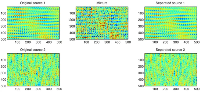
In this very simple experimental setup and for each experiment, we first synthesize the sources using those hyperparameters. During the separation step, we consider that only the synthesized mixture and the hyperparameters are known and we can perform separation through the method presented in section 3.2.2. To this purpose, we can build the spectral covariance tensor Smof each source and then perform separation in the frequency domain as in (10). The sources are recovered through an inverse2-dimensional Fourier transform. It is worth noticing here that the computations only involve element-wise multiplications of500 × 500 images, instead of the inversion of the250000 × 250000 covariance matrix required by the basic GP setup. Results for one example are shown in Figure 1. The average Signal to Error Ratio (SER) obtained on 50 experiments was8dB and the average computing time was less than2s13
.
11CP is also called PARAFAC or CANDECOMP [5].
12This usecase is common in geostatistics: the observed signal is often
modeled as the sum of the signal of interest with a contaminating white Gaus-sian noise. Estimating the value of the target signal through Kriging is hence a special case of GPSS.
Original source 1 100 200 300 400 500 100 200 300 400 500 Original source 2 100 200 300 400 500 100 200 300 400 500 Mixture 100 200 300 400 500 100 200 300 400 500 Separated source 1 100 200 300 400 500 100 200 300 400 500 Separated source 2 100 200 300 400 500 100 200 300 400 500
Fig. 1. GP for the separation of two stationary random fields (D= 2) using GPs. On the left are the original sources. On the center is the mixture and on the right are the estimated sources. A temperature colormap is used : blue indicates large negative values, red indicates large positive values.
5. CONCLUSION
In this study, we have stated the linear underdetermined source sep-aration problem in terms of GP regression and we have shown that it leads to simple formulas to optimally proceed to signals separa-tion with respect to the MMSE criterion. We have furthermore noted connections between GP models and Nonnegative Tensor Factoriza-tions when the mixtures are regularly sampled and the sources are locally stationary. It is noticeable that the proposed framework be-comes equivalent to popular NMF methods when the signals are 1-dimensional.
Setting the source separation problem in such a unified frame-work permits to consider it from a larger perspective where its objec-tive is to separate addiobjec-tive independent functions on arbitrary input spaces that are mathematically characterized by their first and sec-ond moments only. More information on this topic can be found in [9].
6. REFERENCES
[1] P. Abrahamsen. A review of Gaussian random fields and cor-relation functions. Technical Report 878, Norsk Regnesentral, Oslo, Norway, April 1997.
[2] J.-F. Cardoso. Blind signal separation: statistical principles.
Proceedings of the IEEE, 90:2009–2026, October 1998. [3] A. T. Cemgil, S. J. Godsill, P. H. Peeling, and N. Whiteley.
The Oxford Handbook of Applied Bayesian Analysis, chapter Bayesian Statistical Methods for Audio and Music Process-ing. Number ISBN13: 978-0-19-954890-3. Oxford University Press, 2010.
the experiment for50 × 50 signals and obtained an average 4.2dB SER for 0.5s average computing time, compared to 5.7dB for exact inference in ap-proximately45s.
[4] A.T. Cemgil, P. Peeling, O. Dikmen, and S. Godsill. Prior structures for Time-Frequency energy distributions. In Proc.
of the 2007 IEEE Workshop on. App. of Signal Proc. to Audio and Acoust. (WASPAA’07), pages 151–154, NY, USA, October 2007.
[5] A. Cichocki, R. Zdunek, A. H. Phan, and S. Amari.
Nonneg-ative Matrix and Tensor Factorizations: Applications to Ex-ploratory Multi-way Data Analysis and Blind Source Separa-tion. Wiley Publishing, September 2009.
[6] P. Comon and C. Jutten, editors. Handbook of Blind Source
Separation: Independent Component Analysis and Blind De-convolution. Academic Press, 2010.
[7] C. Févotte, N. Bertin, and J.-L. Durrieu. Nonnegative matrix factorization with the Itakura-Saito divergence. With applica-tion to music analysis. Neural Computaapplica-tion, 21(3):793–830, March 2009.
[8] D. D. Lee and H. S. Seung. Algorithms for non-negative matrix factorization. In Advances in Neural Information Processing
Systems (NIPS), volume 13, pages 556–562. MIT Press, April 2001.
[9] A. Liutkus, R. Badeau, and G. Richard. Gaussian processes for underdetermined source separation (to be published). Signal
Processing, IEEE Transactions on, PP(99):1, 2011.
[10] C. E. Rasmussen and C. K. I. Williams. Gaussian Processes
for Machine Learning (Adaptive Computation and Machine Learning). The MIT Press, 2005.
[11] M. Seeger. Gaussian processes for machine learning. Int. J.
Neural Syst., 14(2):69–106, April 2004.
[12] N. Wiener. Extrapolation, interpolation, and smoothing of
sta-tionary time series with engineering applications. MIT Press, 1949.