Plane
mPlane
an Intelligent Measurement Plane for Future Network and Applica on Management
ICT FP7-318627
Cross-Check of Analysis Modules
and Reasoner Interac ons
Author(s): Author names
POLITO U. Manferdini, S. Traverso, M. Mellia FUB E. Tego, F. Matera
ALBLF Z. Ben Houidi
EURECOM M. Milanesio, P. Michiardi
ENST D. Rossi, D. Cicalese, D. Joumbla , J. Auge NEC M. Dusi, S. Nikitaki, M. Ahmed
TID I. Leon adis, L. Baltrunas, M. Varvello FTW P. Casas, A. D’Alconzo
ULG (editor) B. Donnet, W. Du, G. Leduc, Y. Liao TI A. Capello, F. Invernizzi
A-LBELL D. Papadimitriou Document Number: D4.3
Revision: 1.1
Revision Date: 21 Apr 2015 Deliverable Type: RTD
Due Date of Delivery: 21 Apr 2015 Actual Date of Delivery: 21 Apr 2015 Nature of the Deliverable: (R)eport Dissemina on Level: Public
Abstract:
This deliverable presents an extended set of Analysis Modules, including both the improvements done to those presented in deliverable D4.1 as well as the new analysis algorithms designed and developed to address use-cases. The deliverable also describes a complete workflow descrip on for the different use-cases, including both stream processing for real- me monitoring applica ons as well as batch processing for “off-line” analysis. This workflow descrip on specifies the itera ve interac on loop between WP2, WP3, T4.1, and T4.2, thereby allowing for a cross-checking of the analysis modules and the reasoner interac ons.
Disclaimer
The information, documentation and igures available in this deliverable are written by the mPlane Consortium partners under EC co- inancing (project FP7-ICT-318627) and does not necessarily re lect the view of the European Commission.
The information in this document is provided “as is”, and no guarantee or warranty is given that the information is it for any particular purpose. The user uses the information at its sole risk and liability.
Contents
Disclaimer. . . 3
1 Introduction. . . 7
2 Analysis Module. . . 8
2.1 Supporting DaaS Troubleshooting . . . 9
2.1.1 Use Case Reminder . . . 9
2.1.2 Statistical Classi ication Module. . . 9
2.1.3 Results and Lessons Learned . . . 9
2.2 Estimating Content and Service Popularity for Network Optimization . . . 12
2.2.1 Use Case Reminder . . . 12
2.2.2 An Almost Reasoner-less Approach . . . 12
2.2.3 Preliminary Evaluation Results . . . 13
2.2.4 Other Approaches . . . 14
2.3 Passive Content Curation . . . 14
2.3.1 Use Case Reminder . . . 14
2.3.2 Content versus Portal Analysis Module . . . 14
2.3.3 Content Promotion Analysis Module . . . 17
2.3.4 Preliminary Prototype and Online Deployment . . . 17
2.3.5 Evaluation . . . 18
2.4 Service Provider Decision Tree for Troubleshooting Use Cases. . . 20
2.4.1 Use Case Overview . . . 20
2.4.2 Diagnosis Algorithm . . . 21
2.5 Quality of Experience for Web browsing . . . 22
2.5.1 Use Case Overview . . . 22
2.5.2 The Diagnosis Algorithm . . . 25
2.5.3 Cumulative Sum . . . 28
2.5.4 Exploiting Analysis Modules at the Repository Level . . . 29
2.6 Mobile Network Performance Issue Cause Analysis . . . 30
2.6.1 Use Case Reminder . . . 30
2.6.2 System Model Overview . . . 30
2.6.3 Description of the Probes . . . 31
2.6.4 Detection System . . . 32
2.6.6 Evaluation . . . 37
2.6.7 Detecting the Location . . . 39
2.6.8 Detecting the Exact Problem . . . 40
2.6.9 Real World Deployment . . . 43
2.6.10 Practical Implications . . . 44
2.6.11 Limitations . . . 45
2.7 Anomaly Detection and Root Cause Analysis in Large-Scale Networks . . . 45
2.7.1 On-line HTTP Traf ic Classi ication through HTTPTag . . . 46
2.7.2 YouTube QoE-based Monitoring from Traf ic Measurements . . . 49
2.7.3 Statistical Anomaly Detection . . . 54
2.7.4 Entropy-based Diagnosis of Device-Speci ic Anomalies . . . 61
2.7.5 Best and Worst Comparison . . . 64
2.8 Veri ication and Certi ication of Service Level Agreements . . . 69
2.8.1 Bandwidth Overbooking . . . 71
2.9 Network Proximity Service Based On Neighborhood Models . . . 72
2.9.1 Network Proximity Service . . . 74
2.9.2 Simulations on Existing Datasets . . . 77
2.9.3 Deployment on PlanetLab . . . 80
2.9.4 Conclusion . . . 82
2.10 Topology . . . 82
2.10.1 MPLS Tunnel Diversity . . . 82
2.10.2 Middleboxes Taxonomy . . . 92
2.10.3 IGP Weight Inference . . . 96
2.11 Accurate and Lightweight Anycast Enumeration and Geolocation . . . 100
2.11.1 Problem Statement . . . 101 2.11.2 Methodology. . . 102 2.11.3 Validation . . . 107 2.11.4 Measurement campaign . . . 109 2.12 Distributed Monitoring . . . 114 2.12.1 Optimization Models . . . 116 2.12.2 Numerical Experiments . . . 119 2.12.3 Conclusion . . . 120
3 Use-Case Work low. . . .123
3.1 Supporting DaaS Troubleshooting . . . 123
3.3 Passive Content Curation . . . 127
3.4 Service Provider Decision Tree for troubleshooting Use Cases . . . 128
3.4.1 Cooperation between different mPlane instancies . . . 129
3.5 Quality of Experience for Web browsing . . . 129
3.6 Mobile network performance issue cause analysis. . . 131
3.7 Anomaly Detection and Root Cause Analysis in Large-Scale Networks . . . 133
3.7.1 Anomaly Diagnosis. . . 138
3.8 Veri ication and Certi ication of Service Level Agreements . . . 141
3.8.1 Probe Location . . . 143
3.9 Locating probes for troubleshooting the path from the server to the user . . . 144
3.9.1 Ranking probes with respect to their distances to some point of interest . . . 146
3.10 Topology . . . 146
3.10.1 MPLS Tunnel Diversity . . . 146
3.10.2 Middleboxes Discovery . . . 148
3.10.3 IGP Weight Inference . . . 149
3.11 Internet-Scale Anycast Scanner . . . 149
3.11.1 mPlane Work low . . . 150
3.11.2 Challenges . . . 152
1 Introduc on
mPlane consists of a Distributed Measurement Infrastructure to perform active, passive and hybrid measurements. It operates at a wide variety of scales and dynamically supports new functionality. The mPlane infrastructure is made of several components: The Measurement component provides a geographically distributed network monitoring infrastructure through active and passive mea-surements. The Repository and data analysis component is in charge of storing the large amount of data collected and processing it prior to later analysis. The Analysis component provided by the supervision layer allows mPlane to extract more elaborated and useful information from the gath-ered and pre-processed measurements. Finally, the Reasoner component is the mPlane intelligence. It allows for structured, iterative, and automated analysis of the measurements and intermediate analysis results. It orchestrates the measurements and the analysis performed by the probes, the large-scale analysis repositories and the analysis algorithms, actuating through the Supervisor to interconnect with the other mPlane components.
In this deliverable, we update analysis algorithms provided in Deliverable D4.1 [73] (Chapter 2). In particular, we inspect each use cases and discuss improvements and validation results obtained since the early stages of the mPlane project. In addition, we provide an insight into more generic analysis algorithms that are related to network topology and routing.
We next show how each algorithm behaves in the whole mPlane work low (Chapter 3), i.e., how var-ious mPlane modules are used by each algorithm, thereby allowing for a cross-check of the analysis modules discussed in Chap. 2 and the reasoner interactions.
2 Analysis Module
In this chapter, we provide improvements to algorithms irst provided in mPlane deliverable D4.1 [73]. We also provide new analysis algorithms designed and developed to address use-cases, and addi-tional generic algorithms.
The irst series of proposed analysis algorithms are presented in the context of speci ic use-cases. They enable to:
• ind the cause of Quality of Experience (QoE) degradations,
• estimate the future popularity trends of services and contents for network optimization, • classify and promote interesting web content to end-users,
• assess and troubleshoot performance and quality of multimedia stream delivery,
• diagnose performance issues in web and identify the segment that is responsible for the qual-ity of experience degradation,
• ind root cause of problems related to connectivity and poor quality of experience on mobile devices,
• detect and diagnose anomalies in Internet-scale services (e.g., CDN-based services), • verify SLAs.
The second series of analysis algorithms have a generic nature and are therefore presented sepa-rately. They enable to :
• ind measurement probes near some point of interest in the network,
• discover network topology (presence of MPLS tunnels and of middleboxes, inference of IGP weights),
• detect anycast services, enumerate and geolocalize the replicas. These algorithms thus cover a large range of functionalities, such as:
• classi ication and iltering (e.g., of lows, applications, content),
• estimation/prediction (e.g., of Quality of Experience (QoE), popularity, path metrics, topol-ogy),
• detection (e.g., of anomalies, threshold-based changes, interfering middleboxes, hidden rela-tionships between policy rules),
• correlations (e.g. between measurements and QoE, traf ic directions and caches/servers), • diagnosis (e.g., of QoE or web degradation, lack of connectivity).
2.1
Suppor ng DaaS Troubleshoo ng
2.1.1
Use Case Reminder
The goal of this use case is to continuously monitoring the Quality of Experience (QoE) of users accessing content using Desktop-as-a-Service solutions through thin-client connections. When-ever the users experience a poor QoE, the mPlane infrastructure, particularly the Reasoner, acts for troubleshooting its cause and iteratively responds with solutions to improve the overall users’ experience.
2.1.2
Sta s cal Classifica on Module
The role of the reasoner in this use case is to combine the information about the kind of application on top of a RDP connection given by the statistical classi ication module, with the information about the delay on the end-to-end path, so to instrument the network on the troubleshooting action to take to overcome poor QoE issues. Detecting the kind of application on top of the connection is therefore key.
In D4.1 [73], we presented several analysis algorithms we considered to detect the application on top of a given thin-client connection. The main goal there was the design and tuning of an effective statistical classi ication technique which can effectively take advantage of the available features provided by the mPlane probes.
In D3.3 [73], we described the robustness of the statistical classi ication technique based on SVM to network conditions, when the training has been done without considering any network impair-ments, whereas the testing includes traces with impairments such as packet loss and packet delay. In this deliverable we collected all the previous results and carried out additional evaluations, to de-termine the algorithms and the classi ication parameters that allow us to achieve best accuracy, also considering the variety of network impairments that we introduced when collecting the dataset used for training and testing.
We provide a detailed description of the technique and its application to inferring users’ QoE in [29]. Details about the testbed are provided in D5.1 [73].
2.1.3
Results and Lessons Learned
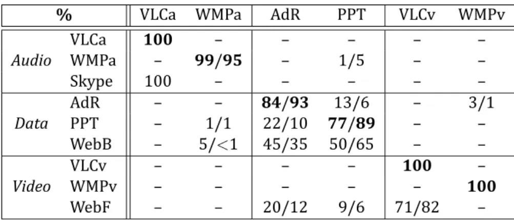
Our results support the idea that considering the SVM algorithm to classify Remote-Desktop-Protocol (RDP) connections over a ten-second time-window allows to infer with high accuracy (up to 99% in some cases) the class of applications that is running over the thin-client connection. Table 2.1 reports on the results achieved with the SVM algorithm on a ten-second time-window. Given that, we focused on the SVM algorithm only for the following experiments.
We investigated how the accuracy of the statistical classi ication techniques changes when the train-ing conditions differ from the testtrain-ing ones. Table 2.2 and Table 2.3 report on the composition of our training set and testing set, respectively.
Our experiments show that the accuracy in detecting lows carrying Video drops by 60% in terms of epochs (40% of bytes) when traces used for training are collected only under the optimal case,
% VLCa WMPa AdR PPT VLCv WMPv Audio VLCa 100 – – – – – WMPa – 99/95 – 1/5 – – Skype 100 – – – – – Data AdR – – 84/93 13/6 – 3/1 PPT – 1/1 22/10 77/89 – – WebB – 5/<1 45/35 50/65 – – Video VLCv – – – – 100 – WMPv – – – – – 100 WebF – – 20/12 9/6 71/82 –
Table 2.1: Classi ication results (percentage) for the SVM algorithm with a ten-second time window. On the left, accuracy by epoch. On the right, accuracy by byte.
Category Network conditions
Apps Duration Bytes down/uplink delay loss
[sec] [MB] [bps] [ms] [%] Audio WMPa 1400 37 6M/1M – – VLCa 1400 35 6M/1M – – Data AdR 1400 63 6M/1M – – PPT 1400 73 6M/1M – – Video VLCv 1400 703 6M/1M – – WMPv 1400 344 6M/1M – –
Table 2.2: Training set composition. AdR stands for adobe reader, while PPT for Powerpoint pre-sentations. VLC is marked as VLCa and VLCv when used for generating audio and multimedia con-tent, respectively. Same consideration holds for WMP.
Category Network conditions Apps Duration Bytes down/uplink delay loss
[sec] [MB] [bps] [ms] [%] Audio WMPa 980 13 6M/1M – – 980 13 3M/512K – – 980 13 1.5M/256K – – VLCa 980 26 6M/1M – – 980 29 3M/512K – – 980 26 1.5M/256K – – Skype 560 15 6M/1M – – Data AdR 980 77 6M/1M – – 980 45 3M/512K – – 980 26 1.5M/256K – – PPT 980 47 6M/1M – – 980 39 3M/512K – – 840 24 1.5M/256K – – WebB 560 83 6M/1M – – Video WebF 560 274 6M/1M – – VLCv 980 498 6M/1M – – 980 277 3M/512K – – 980 153 1.5M/256K – – WMPv 980 302 6M/1M – – 980 265 3M/512K – – 980 153 1.5M/256K – – 140 26 6M/1M 10 – 140 27 6M/1M 20 – 140 19 6M/1M 40 – 140 25 6M/1M 80 – 140 23 6M/1M 120 – 140 21 6M/1M 160 – 140 28 6M/1M – 1 140 20 6M/1M – 2 140 7 6M/1M – 3
Table 2.3: Testing set composition. WebF stands for web pages with embedded Flash videos, WebB for other kinds of web pages. VLC is marked as VLCa and VLCv when used for generating audio and multimedia content, respectively. Same consideration holds for WMP.
i.e., without introducing any impairment on the network, whereas traces used for testing expe-rience a bandwidth squeezing of a factor of four (from a downlink/uplink rate 6Mbps/1Mbps to 1.5Mbps/256Kbps).
We believe this result is important for two reasons. First, it practically shows the rate by which the accuracy of SVM decreases as we force the technique to classify traf ic for which it did not receive any training, both in terms of application and network conditions. Second, it points out that the misclassi ied epochs are actually the ones that carry few bytes, which means that the bandwidth squeezing we apply is so that it alters the values of the features upon which we trained our classi ier, thus altering the behavior of the application inside the thin-client connection, e.g., the multimedia streaming is bursty. As long as the conditions return similar to the optimal ones, such as in the case where the testing traces have a downlink/uplink rate of 3Mbps/512Kbps, the classi ier can keep up and is still able to detect the Video category with an accuracy of bytes around 80%.
To prove this thesis, we further analyzed whether there is room for improvement in the classi i-cation of the testing set in case also the training set includes RDP sessions collected under some forms of network impairments, such as with different bandwidth conditions. Preliminary tests show that the accuracy increases on average of 25% (15%) in terms of epochs (bytes) for multime-dia content. It is worth noting that although these results may justify a motivated service provider to collect training traces in different network conditions to achieve better accuracy, they open to the potential over-specialization (over- itting) of the training set against the testing set.
2.2
Es ma ng Content and Service Popularity for Network
Op-miza on
2.2.1
Use Case Reminder
The goal of this use case is to optimize the QoE of the user and the network load by inferring the expected-to-be popular contents and identifying optimal objects to cache in a given portion of the network. To achieve this goal, we exploit the mPlane architecture in order to collect a large number of online traf ic information requested by the users in several points in the network. The acquired information is exploited in order to predict the content popularity and suggest ef icient caching replacement strategies to the Reasoner.
2.2.2
An Almost Reasoner-less Approach
Differently from other use cases that include troubleshooting and where iterative reasoning is al-most mandatory, the role of Reasoner is basic for the content popularity estimation use case. Indeed it orchestrates the two different analysis modules that monitor and estimate the popularity evolu-tion of contents observed in certain porevolu-tions of the network. The only reasoning task which may require some iteration is the identi ication of the network portions in which contents are labelled as potentially popular.
In its current status, the Reasoner gets the list of expected popular contents from the analysis mod-ules, that run continuously on the repositories, together with information about the network por-tion (i.e., the probe) in which such content was observed. In the scenario of a hiercarchical Content
Figure 2.1: Mean percentage reconstruction error when predicting the future popularity of the video based on the history length (bins represent days). Note how the reconstruction error in-creases as we predict further in the future.
Delivery Network, it would be useful to get the additional knowledge about the location of the con-tents that are expected to be more popular. Consequently, this information could be utilized in order to identify the caching level in the hierarcical CDN at which proactively prefetching the cor-responding content.
2.2.3
Preliminary Evalua on Results
Here we describe the results in inferring the evolution of content requests over time by means of the predictor as described in D4.1 [73]. In particular, we run our prototype on a commercial ISP anonymized trace reporting the requests to YouTube videos watched by a population of 28,000 users.
We adopted a supervised approach, based on heterogeneous mixture models. First, we gathered the models of our target applications by collecting a set of requests for YouTube videos over time (grouped by day) that served as training set. Then, we tested the validity of such models on a subset of 2,000 requests to videos available in our trace.
The goal of this irst evaluation is to assess the ability of the technique to accurately predict the popularity of a given content. We believe this is the irst step into the implementation of caching strategies: it constitues the input for optimizing the cache usage given its size, and for reducing the amount of bytes that we have to transfer if required to be transfered when we know which content should be kept into the cache as it will become popular in the future.
We started investigating the accuracy of our algorithm in predicting the future popularity of the videos, given that the algorithm has seen the irst X data samples of the requests of the videos over time, where X ranges from 11 to 91, with step 5. Fig. 2.1 reports the results in terms of Mean Percentage Error (MPE), that is the ratio between the absolute estimation error (the difference
between the estimated and the real requests) and the number of requests that the video actually gets in the data sample we are trying to predict.
As shown, the algorithm shows good accuracy (MPE is below 20%) in predicting the popularity of the objects in the short-term (e.g., up to the next ten data samples in the future), whereas the accuracy degrades the more we try to predict long-term, especially when the known history is very little (e.g., over 80% of error when the algorithm tries to predict up to 80 data samples ahead in the future, based on the knowledge of the irst 11 data samples).
As future analysis, we plan to assess how the accuracy of the prediction algorithm brings bene it to the overall reduction of the amount of traf ic that has to be transfered over the network across different levels of cache.
2.2.4
Other Approaches
In our ongoing efforts we are analyzing other prediction approaches and evaluating their scalability with respect to the current implementation.
2.3
Passive Content Cura on
2.3.1
Use Case Reminder
We remind that the content curation use case aims at providing a service that helps users identify-ing, fast, relevant content in the web. This use case monitors various probes in the network, detects URL clicks (called user-URLs) out of the streams of HTTP logs observed on the probes, and performs some analysis on these clicks in order to pinpoint the set of URLs that are worth recommending to users.
In D4.1 [73], we presented two of line analysis modules that aim at detecting (1) user-URLs (URLs that were clicked intentionally by users) out of a stream of HTTP logs, and (2) interesting-URLs (user-URLs that are likely to be interesting to recommend to users).
In D3.3 [73], we enhanced our user-URLs detection heuristics and modi ied them to run online at high rates of HTTP requests (up to 5 million per hour). Since this algorithm needs to run continu-ously on HTTP logs streamed from the mPlane probe, we decided to make it a scalable data-analysis algorithm that runs on the repository instead of an analysis module on its own. The output of this algorithm will be user-URLs, together with their timestamps, referrer and a lag saying wether they contain or not a social plugin.
In D4.2 [73], we sketched how we modi ied the structure of the analysis modules to work online, and we present in this document two new analysis modules which rely on the output provided by WP3: (1) the content versus Portal module and (2) the content promotion module.
2.3.2
Content versus Portal Analysis Module
As also described in Sec. 3.3, our use case needs a Content versus Portal module which focuses on discriminating interesting-URLs corresponding to web portals from those pointing to speci ic
con-tent. We use the term web portal or portal-URL to refer to the front page of content providers, which mostly has links to different pieces of content (e.g., nytimes.com/ and wikipedia.org/); whereas a content-URL refers to the web page of, e.g., a single news or a wikipedia article. We thus engineer an analysis module that is a classi ier that distinguishes between web portals and content-URLs. 2.3.2.1 Features
We use ive features to capture both URL characteristics and the arrival process of visits users gen-erate.
URL length. This feature corresponds to the number of characters in the URL. Intuitively, portal-URLs tend to be shorter than content-portal-URLs.
Hostname. This is a binary feature. It is set to one if the resource in the URL has no path (i.e., it is equal to “/”); and to zero, otherwise. Usually, requests to portal-URLs have no path in the resource
ield.
Frequency as hostname. This feature counts the number of times a URL appears as root of other interesting-URLs. The higher the frequency, the higher the chances that the URL is a portal. Request Arrival Process (RAP) cross-correlation. The URL request arrival process is modelled as a vector in which each element counts the number of visits in ive-minute bins. We noticed that users often visit portal-URLs following some diurnal periodic pattern. Intuitively, the more the re-quest arrival process signal of a given URLs is “similar” to that of a well known portal, the higher the chances that the URL corresponds to a portal. To capture such a similarity, we compute the maximum cross-correlation between (1) the request arrival process of a tested URL and that of (2) well-known portals (e.g., www.google.com or www.facebook.com). The cross-correlation, a well known operation in signal processing theory, measures how similar the two signals are, as a function of a sliding time lag applied to one of them. The higher the value of the maximum of the cross-correlation, the larger the chance of a URL being a portal.
Periodicity. This is a binary feature that captures the fact that users visit portals with some period-icity. We use the Fast Fourier Transform (FFT) on the discretized aggregate visit arrival process for a given URL. If the visit arrival process shows one-day periodicity (principal frequency of 1/24h), then we set periodicity to one; zero, otherwise.
Note that the last two features would intuitively work only for popular-enough portals that get enough clicks to exhibit the periodic diurnal cycle. However, as we will see in Sec. 2.3.3, we only promote content that has captured a suf icient amount of attention. As such, unpopular portals are less likely to be promoted.
Finally, we opt for a supervised machine learning approach to build a classi ier based on the above features. Given the heterogeneity of the URL characteristics, we choose the Naive Bayes classi ier. This classi ier is simple and fast, which is important for online implementation. As we will see, it achieves good performance, not calling for more advanced classi iers.
2.3.2.2 Accuracy
To evaluate the accuracy, we observe a stream of interesting-URLs (extracted from http logs of a commercial ISP) and by visiting such URLs, we manually pick among them 100 content-URLs and 100 portal-URLs. We use this set for both training and testing. In particular, we randomly divide the 200 URLs into two sets: two thirds of the URLs for training and one third for testing. We use a ten-fold validation, averaging results from 10 independent runs.
Interesting URL i OFF-Thread |Observations(i)| >= W Yes No ci = OFF-CL(i), add (i, ci) to K End. Update Observations(i) ON-Thread i in K Yes No Get outcome ci End. ci = ON-CL(i)
Figure 2.2: Work low of the online content vs. portal URL classi ier
We build several combinations of features and choose the one that shows the best tradeoff be-tween precision and recall. Our results show that we achieve the best accuracy by combining the URL length and the periodicity. This combination achieves 100% precision and 93% recall for web portals, and 94% precision and 100% recall for content-URLs, which translates into an overall ac-curacy of 96%. This means that we have a very high precision whenever we tag a URL as Portal. However, around 6% of what we tag as content-URLs are in reality portals.
2.3.2.3 Online Classifier
Our analysis module needs to run online, that is to decide as soon as it is seen whether an interesting-URL is a content-interesting-URL or a portal-interesting-URL. We now describe the online version of the classi ier we use to distinguish content-URLs from portal-URLs. It takes as an input a stream of tuples <interesting-URLs, timestamps>, and it outputs binary labels as <interesting-<interesting-URLs, label (content-URL/portal-URL)>.
Despite we achieve the best accuracy when combining the features URL-length and periodicity, this latter complicates the design of the online classi ier, as it has to observe each interesting-URL for some time, e.g., a week. Therefore, we design the online classi ier based on the observation that the features can be split in two categories: those that analyze the structure of the URL (URL Length and hostname), and those that rely on the visit arrival process (RAP cross-correlation, periodicity and frequency as hostname). For the irst set we can take decisions on-the- ly, while the latter requires to collect observations for a few days before being able to correctly take a decision. Thus, we split the classi ication work low into two threads, as depicted in Fig. 2.2. The left thread, named
OFF-Thread, collects observations for the features RAP cross-correlation, periodicity and frequency
as hostname. As soon as the interesting-URL i has been observed for enough (W ) times (being each observation corresponding to a user visit to i), i is classi ied using features URL-length and periodicity (the most accurate in our experiments, method OFF-CL in Fig. 2.2), and the outcome ci
is stored in the Knowledge Database, K. The right thread, named ON-Thread, performs classi ication on-the- ly based on the per-URL “online” features (method ON-CL in Fig. 2.2). In particular, we test our classi ier on a groundtruth trace that we build by visiting the top 100 websites in Alexa ranking. We observe that combining URL length and hostname gives us a 93% accuracy on the groundtruth
trace.
Therefore, for every interesting-URL i, we irst rely on the OFF-CL result, if available, i.e., we verify the presence of i in K. Otherwise, we use the faster, but less precise, ON-CL result.
2.3.3
Content Promo on Analysis Module
This analysis module is useful to decide which content-URLs to promote and show to the users, it takes as an input content-URLs, computed by the previous analysis module. In the current status of the use case, we test four different promotion mechanisms to use for as many sections (or tabs) in the front end website that we built for a irst prototype of our use case.
Hot. This mechanism is an adaptation of Reddit’s Hot ranking algorithm [109], which promotes URLs that are both popular and recent. The algorithm behind Reddit’s Hot ranking assigns each URL a score based on users’ votes. We replace such votes with the number of visits, and modify Reddit’s formula to obtain the following:
Score = log(Nviews) +
Tf irst− Tstart
TP
Nviewsreports the number of views, Tf irstis the time corresponding to the irst time the
content-URL has been observed (i.e., visited), and Tstartis the time corresponding to an absolute reference,
i.e., the start of the system. Finally, TP represents the normalization factor that we use to de ine a
”freshness period”, and that we set to 12 hours. Intuitively, this formula inds a balance between the content popularity (the number of views) and its freshness (its age with respect to the absolute reference). When a content-URL stops getting attention, its ranking starts decreasing due to its age. Top. This mechanism produces a simple ranking of URLs depending on the number of views. In the current version, in order to keep the memory usage of the system steady, this ranking accounts only for one week of history.
Fresh news. This mechanism focuses on one category of content-URLs, namely news, and aims at promoting the freshest news seen in the network. In order to detect if a content-URL corresponds to a news, we rely on a prede ined list of traditional news media websites in Italy: if the hostname of a content-URL belongs to this list, and if the content-URL has never been seen before, we tag it as news and promote it as fresh news. We construct the list of news websites by observing Google News, a popular news aggregation and indexing system that uses an active approach based on web-crawlers to collect and promote news. More precisely, Google servers regularly query a prede ined set of popular news portals, looking for new articles to push on the front page [38]. To construct the list of news portals, we crawl the Google News front page every 20 minutes for a period of one week, looking for new websites. This allowed us to obtain more than 500 distinct news websites. Live news stream. It simply promotes the news, as de ined earlier, as soon as they get attention from users in the network, i.e., in a continuous manner.
Finally, when a content-URL receives a visit, this analysis module updates the score of the URL and its number of views. The content promotion analysis module periodically recomputes the ranking and updates, if necessary, the database used to store the contents in the Hot and Top categories.
2.3.4
Preliminary Prototype and Online Deployment
Figure 2.3: Screenshot of the website running the Content Curation prototype available at http: //tstat.polito.it/netcurator/
By feeding the online algorithms described in previous sections with a live stream of HTTP requests that has been made available from Politecnico di Torino, we deploy a complete prototype of the system running in an actual operational network.
Thanks to a Tstat probe installed at the egress vantage point of the campus network and obtain HTTP requests generated by around 15,000 users, i.e., students and personnel regularly accessing the Internet. On average, users generate 7M HTTP requests per day. Out of these the system extracts on average 55,000 user-URLs, corresponding to 5,000 interesting-URLs. The backend server of the system receives the stream of HTTP requests and processes it to detect, irst, interesting-URLs, then, content-URLs, and, inally, among those the URLs to promote on the website, that we named NetCurator: http://webrowse.polito.it/.
As depicted in Fig. 2.3, the website consists in four tabs, one for each promotion method. Each tab contains a content feed whose design is inspired by the “wall” implemented in popular social networks such as Facebook and Twitter, and URLs that make it to the feed are presented with a preview image, a title, and a description when available. In our ongoing efforts we are working to make all the system components mPlane-compliant.
2.3.5
Evalua on
This section evaluates various aspects of our prototype. First, to evaluate its ef iciency in processing HTTP logs, we apply it on the passive HTTP log trace that have been collected in a commercial European ISP. This trace reports the HTTP activity of 19,000 users regularly accessing the Internet
1M
2M
3M
4M
00:00
5:00
10:00
15:00
20:00 24:00
0
13
26
39
52
HTTP requests
Processing Time [min]
Time
HTTP requests
Processing Time
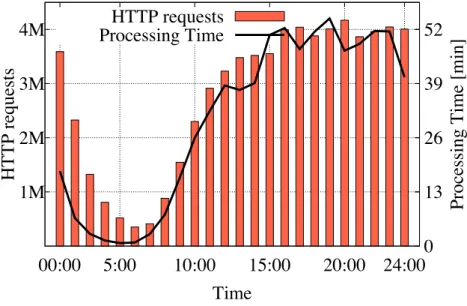
Figure 2.4: HTTP requests rate (left y axis) and processing time (right y axis) over time for one day extracted from HTTP-ISP
through ADSL/FTTH access technologies. The trace, that we name HTTP-ISP, reports in total more that 190M HTTP requests that users have generated over a period of three days of April 2014. As we described in D4.2, Sec. 2.3.5.1 evaluates the performance of the prototype when we feed it with the passive trace HTTP-ISP. Finally, Sec. 2.3.5.2 focuses on the Fresh News tab (see Sec. 2.3.4 for a detailed description) to see how ef icient it is in detecting fresh news.
2.3.5.1 Performance
In order to understand the performance of the prototype, we evaluate how it behaves when it pro-cesses HTTP-ISP, whose per-hour rates of HTTP requests are much larger with respect to the live deployment we described in Sec. 2.3.4. We show how the prototype performs against the day in
HTTP-ISP that has the largest peak hourly rate of HTTP requests. We split the one-day trace in
1-hour long sub-traces, and use them to feed our prototype. For each 1-hour, we measure the time that the prototype spends to end the processing. For this experiment, we run the prototype on a six-core Intel 2.5GHz CPU and 32GB RAM server.
Fig. 2.4 reports the amount of HTTP requests (left-hand y axis) and the corresponding processing time (right-hand y axis), for all the 1-hour long bins in the day of HTTP-ISP. The igure shows that the implementation of the prototype is able to inish all the one-hour traces in less than one hour. This demonstrates that it can sustain the processing of such large rates of HTTP requests on a rather standard server like the one we picked above. Finally, we note that its memory footprint is minimal, as less than 5% of memory was used throughout the experiment.
2.3.5.2 How fast can our Content Cura on system Detect Content?
Finally, this section assesses what we expected to be a nice property of our prototype when we designed it: fast discovery of Internet content. Indeed, if Google News has robots that actively look
for new content to index, our system can rely on an “army” of users who explore the web looking for fresh news. In this section, we set the bar high and leverage our online deployment to compare the two approaches and assess how fast is our content curation system in discovering news content. Since the content in both “Fresh news” and Google News relies on the same list of traditional news providers, the only difference between them is that ours uses the crowd of users to discover content, while Google’s uses robots.
To compare the two approaches, each time our prototype promotes a content-URL to “Fresh news”, we check if Google has already indexed it,1and if it has, we measure since when (this “age” is an information available below each link returned by Google Search). We run this experiment for a period of one day (after that, Google has banned our IP network because of the extensive probing). We observe that despite the small sample of users that our prototype has in its current live deploy-ment, it was able to ind few not-yet indexed news URLs. Fig. 2.5 shows the number of not indexed news in each hour of the day. We put this number in perspective with the total number of “Fresh news” per hour. The igure shows, not surprisingly, that the more views we have, the higher the chances that we ind not-yet-indexed content.
We conclude that with such a small number of users, our content curation system cannot compete on the speed of content discovery, especially when the space of news to discover is limited (a pre-de ined list of news portals). Inpre-deed, our analysis of the age of news shows that in 96% of the cases, our prototype is more than 1 hour later than Google News in discovering a news URL.
However, an interesting observation is the age of the news articles that are consumed by users in the network (and that are therefore promoted by the prototype). In fact, although platforms like Google News promote on their front page very fresh news (from few minutes to two hours old), our experiment shows that 44% of the consumed news were published one to several days before (according to when they were irst indexed by Google). This means that although content freshness is important for news, a big portion of news article are still “consumable” one to few days after their publication.
2.4
Service Provider Decision Tree for Troubleshoo ng Use Cases
2.4.1
Use Case Overview
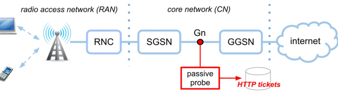
The reference scenario, as depicted in Fig. 2.6, is based on a typical SP’s infrastructure. The SP has built and runs a completely private instantiation of the mPlane infrastructure. This means that all the probes, the repository, the supervisor and the reasoner are under the exclusive control of the SP.
In order to evaluate the QoE of a speci ic service (e.g., video streaming) a continuous monitoring infrastructure built upon a set of passive probes is used. Passive probes are placed in multiple van-tage points and extract from traf ic lows data useful to estimate the QoE. For instance, the average throughput per low or the Round Trip Time can be usefully used to build performance parameters associated to the monitored service. Besides the set of passive probes, the reference scenario also considers the availability of a set of active probes. The active probes are located directly behind a subset of access nodes (e.g. DSLAMs, OLTs, etc.), within the PoP site and next to the Internet
Gate-1We use several instances of a headless browser to do a “site:” search on Google Search for each news-URL the pro-totype detects.
0
2
4
6
8
10
7:00
13:00 18:00 23:00
05:00
0
280
560
840
1120
1400
Not-indexed News-URLs
News-URLs
Time
Not-indexed News-URLs
News-URLs
Figure 2.5: Number of not-indexed news-URLs (left y axis), and number of news-URLs (right y axis) during one day (Online deployment)
ways. These probes are able to perform active measurements: for instance, Ping/traceroute or actively requesting video contents and taking measures from Over The Top services (e.g. YouTube). The active probes work on demand, following triggers coming from the Reasoner (through the Su-pervisor).
2.4.2
Diagnosis Algorithm
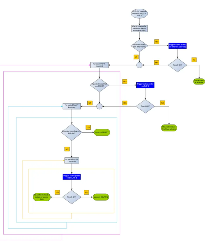
Fig. 2.7 depicts the diagnosis algorithm.
The Analysis module is the trigger of the overall troubleshooting process. When the performance measures are below the threshold, a ”NOT OK” response is sent to the Reasoner which starts the process to ind the cause of the problem, according to the actions described in the graph. The al-gorithm is described in detail in deliverable D4.2 [73]. It is based on a very basic decision tree that highlights the iterative interaction with the probes. More sophisticated algorithms or machine learning approaches could be used to speed-up the process and reduce the communication with the probes. Anyway, at this stage, we prefer to propose an algorithm that is easy to understand for people working in network operation teams because it is based on an expert-driven approach, the same they use daily to solve the issues. In this way, the purpose of each step of the algorithm is clear. At the same time, the overall process, including the communication with the probes, is completely automatic, boosting the ef iciency of the analysis.
Currently, part of the analysis module has been implemented. Speci ically, the software that ag-gregates the QoE parameters measured by the passive probes is available. The aggregation is per-formed on a per-DSLAM basis, in order to have a suf icient granularity to trigger the Reasoner pro-cess. The QoE parameters taken into account are the bandwidth and the Round Trip Time (RTT). The passive probes calculate these quantities for each session and store the values into the Reposi-tory. The analysis module takes these values, aggregates them per-DSLAM, and calculates the aver-age. The obtained result is compared to a pre-de ined threshold: if the result is below the threshold,
Figure 2.6: Reference scenario
the analysis module interprets it as a QoE degradation and triggers the Reasoner process to ind the cause of the problem. An example of the average bandwidth per-DSLAM is shown in Fig. 2.8, where the value is calculated every 10 minutes. After each calculation, the analysis module sends a feed-back to the Reasoner process: ”OK”, if all the DSLAMs are over the threshold, ”NOT OK”, if one or more DSLAMs are below the threshold. In both cases, the values are sent to the Reasoner.
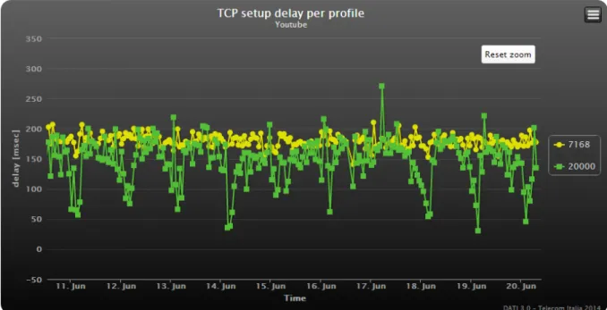
Fig. 2.9 shows an example of RTT calculated from the sessions of a speci ic DSLAM. In this case, the values are classi ied also on the basis of the pro ile of the access line. This option can be enabled also for the bandwidth calculation.
The RTT is primarily useful to detect rerouting events that move the traf ic on longer paths. These events can be within the SP’s network (e.g., a link fault on the primary path) or can be due to the Content Provider that starts serving the content from a different site. The bandwidth gives infor-mation that partially overlaps with RTT, but it additionally gives hints on packet loss events, that can be due, for example, to network congestion.
2.5
Quality of Experience for Web browsing
2.5.1
Use Case Overview
The QoE for Web browsing use case aims at identifying the root cause of a poor performance in browsing (i.e., high Web page loading time). The identi ication of the root cause exploits measure-ments taken on distributed probes, both actively and passively. The probes passively records HTTP time measurements from an instrumented headless browser (i.e., phantomJS) and couples them
Figure 2.7: Diagnosis algorithm
with the log collected at the TCP level by Tstat. The probes perform then active measurements (namely, Ping and Traceroute) over the collected IP addresses. The result of the diagnosis is an in-formation on the location of the root cause (e.g., local host / lan, home gateway, remote web server, and so on).
In D4.1 [73], we presented the preliminary algorithm and scenario aiming at identifying the seg-ment that is responsible for the high Web page loading time. In D4.2 [73], we further detailed the
Figure 2.8: Average bandwidth aggregated per-DSLAM
Symbol Metric Passive or Active
Tnhop RTT to the nthhop Active
∆n T
(n+1)hop− Tnhop Simple Computation
Tidle Client idle time Passive
Ttot Total web page downloading time Passive
TDN S DNS response time Passive
Ttcp TCP response time Passive
Thttp HTTP response time Passive
Table 2.4: Metrics used in the diagnosis algorithm for the Web QoE Use Case
work low for the iterative analysis at the Reasoner level.
Now we present the complete picture, relying both on the probe measurements and on the reposi-tory data.
2.5.2
The Diagnosis Algorithm
We remind all the collected metrics that are exploited by the diagnosis algorithm in table 2.4. We can identify different segments where the problem of a high page loading time could be located (each segment is indicated with a question mark in Fig. 2.10, taken from Deliverable D4.2 [73]): (1) at the probe side, i.e., local probe, local network, gateway; (2) at the domain side, i.e., middle boxes (if any), DNS server; (3) the backbone network; and (4) the remote web server.
The main diagnosis algorithm is described in Algorithm 1.
Lines 1-9 are executed on data coming from the single probe to infer the status of the probe (e.g., CPU usage) and browser level measurements2(lines 3-9).
If the total time of retrieving all the objects in the web page is under a certain threshold (test on line 3) then we investigate the remote web server part of the path, namely the page dimension, the time for setting up a TCP connection and the time taken to resolve the URL. On the contrary, if the total time of fetching all the items on a web page is high, there can be three distinct cases: all the other devices in the same local network are experiencing some problems, none of the other devices is experiencing any problem, and just some of the other devices are experiencing some problems (lines 11-34).
In case all the different devices are experiencing some problems (lines 12-18) the algorithm can directly exclude that the problem is due to the remote server (assuming that not all the devices are contacting the same remote server). The algorithm assumes then that most probably the problem is located close to the devices (otherwise probably not all the devices would experience problems) and thus begins this diagnosis phase by checking the gateway and the local network (Algorithm 2), if the problem is neither in the gateway nor in the local network, it checks the middle boxes (Algo-rithm 3), and inally, if the problem is neither in the middle boxes, it concludes that the problem is in the backbone network (probably in the portion of the backbone that is close to the local network, given that all the local devices are traversing it).
Let us dive into the check-gateway-lan algorithm (Algorithm 2). First of all (lines 1-5), the algo-rithm veri ies if the CUSUM [97] (see Sec.2.5.3) applied to the T1hop(where 1hop is the gateway) exceeds an appropriate threshold. If this is the case, this can justi ied by either the fact that the lo-cal network is congested or by the fact that the gateway is overloaded and the PING response time is “anomalous”. To discriminate between this two cases the probe also checks the CUSUM applied to Tp(where p is another device of the network) and if it is “anomalous” too, it concludes that the
problem resides in the local network, which is probably congested, otherwise it concludes that the problem is in the gateway, which is probably overloaded.
Else, if the T1hopis “normal”, the algorithm cannot yet exclude the overloaded gateway case (be-cause the relation between the ping response time and the machine load is not always signi icant, as usually PING messages are directly managed by the network card) and performs a check on the CUSUM applied to ∆1. Note that this metric, from a practical point of view roughly represents the sum of the time needed to traverse the gateway, the time needed to go through the irst link out-side the gateway, and the time required by the second hop to process the PING request. If this is “anomalous”, the algorithm also checks the CUSUM applied to ∆2and in case it is “anomalous” too it concludes that there is congestion on the irst link outside the gateway, which is reported as back-bone network problem (note that if there are middle boxes the algorithm instead proceeds to the next phase), otherwise it concludes that the problem is in the gateway that is overloaded.
In case ∆1results to be “normal”, the algorithm can exclude the overloaded gateway case, and pro-ceeds by checking the middle boxes, if any. The veri ication of the middle box (Algorithm 3) is based on a process that is very similar to the one used to check the gateway. The algorithm checks the CUSUM applied to Tnhop(where n is the middle box). If this is “anomalous”, it can conclude that the 2The current implementation of the probe with the headless browser does not allow the capturing of DNS times and idle times. The irst, because we can not distinguish DNS requests from the Tstat logs, the second because on a headless browser there is no rendering of the web page. This choice was driven by the need to lighten the probe on low-power hardware, and to deploy the probe as a standalone box on which take the measurements. User interaction (i.e., the explicit warning that a high page loading time is experienced) is always collected by a “full browser” plugin.
Algorithm 1 Web QoE diagnosis main algorithm
1: ifTidle
Ttot > ψ1or CP U usage > ψ2then
2: return local client ▷otherwise exclude local client
3: if Thttp< ψ3then ▷exclude any kind of network problem
4: if P ageDimension > ψ4then
5: return page too big
6: if Ttcp> ψ5then
7: web server too far
8: if TDN S> ψ6then
9: return DNS ▷otherwise exclude the DNS problems
10: else ▷the problem is somewhere in the network
11: check other probes in the local network
12: switch Do they have problems? do
13: case They are ALL experiencing problems ▷exclude the remote server
14: if CHECK GW/LAN then
15: return GW/LAN
16: if CHECK MiddleBox then
17: return Middle Box ▷exclude gateway and local network
18: return network ▷the problem can be only in the net (near portion)
19: case NONE is experiencing problems ▷exclude GW, LAN, Middle boxes
20: if CU SU M (Thttp− Ttcp) > ψ6then ▷reload page and check again
21: return remote web server
22: else
23: return network ▷the problem can be only in the net (far portion)
24: case SOME are experiencing problems ▷ exclude gateway, local network, middle box, and almost certainly
the remote server
25: return network
26: case No Other Probe Available
27: if CHECK GW/LAN then
28: return GW/LAN
29: if CHECK MiddleBox then
30: return Middle Box ▷exclude gateway and local network
31: if CU SU M (Thttp− Ttcp) > ψ6then ▷reload page and check again
32: return remote web server
33: else
34: return network ▷the problem can be only in the net (far portion)
problem is in the middle box, otherwise it checks if any anomaly is present in ∆n: if not, it excludes
the middle box and, in case, goes to the next middle box, otherwise it also check ∆n+1, concluding
that the problem is in the middle box, if the latter is “normal”, or in the congested network, if not. Note that this phase is apparently simpler than the one responsible for checking the gateway, just because it can exploit all the information already obtained from the previous phases: if the algo-rithm cannot locate the problem neither in the gateway and local network, nor in the middle boxes, it concludes that the problem resides in the near portion of the backbone network.
Back at the main algorithm, let us analyze now the case in which none of the other devices of the local network is experiencing any problem (Algorithm 1, lines 19-23). In this case, we can easily exclude the gateway, the local network, and the middle boxes, restricting the possible results to either the remote web server or the backbone network. Hence, the irst check is performed on the remote server (that is assumed to be more probable than the backbone network, given that the only device that is experiencing problems is the one navigating that remote server).
Algorithm 2 CHECK GW/LAN
1: if CU SU M (T1hop) > ψthen
2: if CU SU M (Tp) > ψthen
3: return Local
4: else
5: return GW ▷optionally I can ask another probe to verify
6: else
7: if CU SU M (∆1
) > ψthen
8: if CU SU M (∆2) > ψthen
9: return Network (backbone) congestion
10: else
11: return GW
▷exclude GW and LAN
Algorithm 3 CHECK MiddleBox
1: to apply for each middle box
2: consider middle box n ▷for the irst middle box after the gw, n = 2)
3: if CU SU M (Tnhop) > ψthen
4: return MiddleBox n ▷note that CU SU M (∆n−1) < ψ
5: else
6: if CU SU M (∆n
) > ψthen
7: if thenCU SU M (∆n+1
) > ψ
8: return network congestion
9: else
10: return Middle box n
11: else
12: check next Middle Box
▷exclude MiddleBoxes
“anomalous” or not3. If yes, the algorithm concludes that the problem is located in the remote web server, otherwise that it is located in the backbone network.
If some of the local network devices are experiencing some problems and some are not (lines 24-25), the algorithm directly concludes that the problem is in the backbone network.
Note that, despite the quite complicated description of the algorithm, the number and the type of the operations made by the probe make it suitable for being used on a background task, without sig-ni icantly affecting system performance. Indeed all the checks are performed by either simply com-paring some passive measurements to a threshold or computing the CUSUM statistics (CUSUM is well-known for being suitable for all kind of real-time applications) and comparing it with a thresh-old.
Finally (lines 26-34), if no other probe are available in the local network, then we fall back to the case in which all probes in the network are experiencing problems.
2.5.3
Cumula ve Sum
To discover anomalies, we exploit a well knows technique named Cumulative Sum (CUSUM) [97], also known as cumulative sum control chart. It is a sequential analysis technique,q typically used for monitoring change detection. Let us suppose to have a time series, given by the samples xn
from a process, the goal of the algorithm is to detect with the smallest possible delay a change in
3Note that this metric roughly represents the time needed by the remote server to process the HTTP GET request, being Ttcpalmost independent on the server load, when the server is not in the local network
the distribution of the data. The assumption of the method is that the distribution before and after the change (fθ1(x)and fθ2(x)) are known. As its name implies, CUSUM involves the calculation of
a cumulative sum, as follows:
S0= x0 Sn+1= ( Sn+ log (fθ2(x) fθ1(x) ))+ (2.1)
The rationale behind the CUSUM algorithm is that, before the change the quantity log(fθ2(x)
fθ1(x) )
is negative, whereas after the change it is positive: as a consequence, the test statistics Snremains
around 0 before the change, and it increases linearly with a positive slope after the change, until it reaches the threshold ξ when the alarm is raised.
Note that the assumption about the knowledge of the two distributions fθ1(x)and fθ2(x), implies
that CUSUM is only able to decide between two simple hypotheses. But, in case of network problems we cannot suppose that the distribution after the change is known (usually neither the distribution before the change is known). This implies the need of using the non parametric version of the algorithm [97], which leads to a different de inition of the cumulative sum Sn. In more detail in this
work we have used the non parametric CUSUM (NP-CUSUM), in which the quantity Snis de ined
as:
S0 = x0
Sn+1= (Sn+ xn− (µn+ c· σn))+
(2.2) where µnand σnare the mean value and the standard deviation until step n, while c is a tunable
parameter of the algorithm.
As far as the estimations of µ and σ are concerned, we can use the Exponential Weighted Moving Average (EWMA) algorithm de ined as:
µn= α· µn−1+ (1− α) · xn
σn= α· sigman−1+ (1− α) · (xn− µn)2
(2.3) where α is a tunable parameter of the algorithm.
2.5.4
Exploi ng Analysis Modules at the Repository Level
The analysis modules computing statistical distributions and values at the repository level are pro-vided as tools to check this (see Sec. 3.5). At the repository level, the Reasoner can check:
• historical values of the RTTs to a particular IP address, • changes in the traceroutes to the same host,
• other probes in the same network (i.e., same 1st hop in traceroute: same gateway), • other probes in the same area (i.e., geo-location tools),
• particular segments with high RTTs (e.g., traceroute from different probes intersecting two subsequent hops),
• the target web server against different probes geographically distributed,
In order to present consistent data to the Reasoner, (i) cleaning, (ii) normalization, and (iii)
trans-formation are performed at the Repository level. The irst is the process of detecting and correcting
corrupt or inaccurate records, caused, for example, by user entry errors or corruption in transmis-sion or storage; the second aims at reducing data to its canonical form, to minimize redundancy and dependency; and the third converts a set of data values from the data format of the source into the data format of the destination system (in our case we store JSON objects into HDFS).
After this preprocessing, the Repository presents the capability of computing simple statistic func-tions to be applied to the collected data (mean value, standard deviation, median, etc.) with differ-ent time granularities (e.g., hour, day, week, month), as well as the capability to cluster the collected data about users, lows, servers, ISP or geographical locations. As a result, we can dive in more de-tails in all cases in which the main algorithm returns a generic “network” problem.
As for now, all the analysis modules on the Repository must be explicitly invoked, while our goal is to automate them as soon as new data arrive from the probes (i.e., moving from batch processing to stream processing).
2.6
Mobile Network Performance Issue Cause Analysis
2.6.1
Use Case Reminder
This scenario focuses in identifying the cause of possible problems that are related to experiencing video-on-demand on mobile devices.
Video stream delivery on mobile devices is prone to a multitude of faults originating either from device hardware constrains, failures in the wireless medium or network issues occurring in differ-ent points along the data path. Although well established video streaming QoE metrics such as the frequency of stalls during playback are a good indicator of the problems perceived by the user, they do not provide any insights about the nature of the problem nor where it has occurred. Quantifying the correlation between the aforementioned faults and the users’ experience is a challenging task due the large number of variables and the numerous points of failure. To address this problem, we are developing a root-cause diagnosis framework for video QoE issues. With the aid of machine learning, our solution analyzes metrics from hardware and network probes deployed on multiple vantage points to determine the type and location of the problems.
2.6.2
System Model Overview
In a typical scenario where a user streams a video on a mobile device from a popular service like YouTube, a request to the content server is made to receive the video data. When the server re-ceives the request, it sends the data either directly from the content server or through a Content Distribution Network (CDN). Then the data stream enters the Internet Backbone until it arrives to the client’s ISP network. If the client is connected on a cellular network, then the data is delivered to the mobile from the client’s serving cellular tower. If the device is connected from a Wi-Fi home network, then the video is delivered over a broadband access link to the home gateway and inally to the mobile device.
Each hop of the data path may suffer from impairments that can affect the smooth delivery of the video and therefore the user’s experience. Congestion or bandwidth bottlenecks in the local or re-mote network segments, high load on the devices and problems in the wireless medium are some of the most signi icant issues that cumber the performance of video streaming services and contribute in the user’s QoE degradation.
To detect the types of failures that may cause issues during the video playback, we need to place measurement probes at multiple vantage points (VP) so that we can extract performance metrics from different segments and devices along the path. In an ideal con iguration, probes in all the intermediate devices of the path would provide us with measurements regarding the performance of each individual hop.
However, our approach only requires probes at the mobile device, the home router and the content server. We only use these three points as they allow us to capture issues at the boundaries of each of the three important entities in the video delivery path, the user, the ISP and the content provider. With the mobile and the server probes we are able to collect measurements from both the data receiver and sender’s point of view, which correspond to the endpoints of the connection. The home gateway acts as an intermediate VP capable of acquiring metrics from both the local (LAN) and the wide are network (WAN).
In this work, we focus on understanding the contribution of each VP when detecting problems, their type and location and with what accuracy. We also examine the bene its of combining the data from multiple VP when they cooperate and in which scenarios the combination becomes more bene icial.
2.6.3
Descrip on of the Probes
Since the majority of popular video streaming services deliver content over TCP, statistics of TCP lows are key to analyze the network metrics that could reveal problems deeper in the data path. For the purpose of collecting network metrics, we use the TCP statistics tool tstat. Tstat is capable of periodically generating logs based on statistics extracted from the TCP lows that are observed during runtime, such as delay, re-transmissions, window size and time-outs.
The mobile probe. We developed the mobile probe for the Android platform to measure TCP, network interface and hardware metrics and monitor the system’s log for events relevant to the progress of the video sessions and the performance of the playback. The probe is capable of col-lecting three types of metrics, network, hardware and system events.
In more detail, the network metrics that we obtain are the parameters and TCP low statistics col-lected by tstat. From the logs created by the tool we extract 113 metrics and statistics about a single TCP low, including RTT, number of packets, low duration, window sizes, out-of-order packets and re-transmissions.
In addition to tstat, the probe is con igured to log all incoming and outgoing packets at the NIC as well as the errors and dropped packets. The hardware metrics are required for providing informa-tion about the available resources on the device and the state of its connectivity. These metrics are directly correlated to the performance of video streaming and video decoding.
The hardware metrics on the smartphone capture the percentage of CPU utilization, the amount of free system memory in KB and the wireless connectivity status (RSSI). These three parameters give us important information about the hardware state and the amount of load of the device. Other hardware parameters were also considered but we concluded that the ones presented here are the
most signi icant for describing the device’s performance.
Finally, the mobile probe monitors the system event log for information about the start-up delay of the video and the number and duration of rebuffering events. The rebuffering events indicate the depletion of the video buffers that force the playback to pause until the buffers ill up to a certain threshold. These interruptions experienced by the user, are indicators of problematic sessions and the QoE of the user. Except from stalls due to buffer outages we also consider stalls caused by high load on the device that do not allow the proper decoding of the video stream.
The router probe represents the irst hop of the connection between the device and the server. It resides on the edge of both the LAN and WAN segments and therefore it is an important VP for measuring the performance of both sides. Although in our model we use a home router, in real scenarios it could be placed at any point that provides wireless connectivity such as a cellular base station.
The router probe con igured to capture network metrics in a similar manner to the mobile probe. There is an instance of tstat running on the device and at the same time the probe logs statistics regarding the number of packets seen arriving or leaving the wireless interface and the number of packets that were dropped. In addition, the probe is capable of monitoring the RSSI of the wireless interface of the connected clients.
The server probe. The selection of the server for the placement of the probe allows the mea-surement of lows from multiple clients connecting from a large number of devices. It additionally serves as a measuring point with a view from the endpoint of the connection that helps identify issues like bottlenecks and slow response times.
The probe on the server is as well instrumented with tstat for measuring network parameters and with a tool to monitor and log statistics about the machine’s NIC using the same approach as the router probe.
In this section we presented probes that were developed to be compatible with different platforms depending on the architecture and operating system of the host device. Hence, in our system we have versions of these probes for Android, OpenWRT and Linux.
2.6.4
Detec on System
It is dif icult to measure the correlation between QoE metrics such as playback stalls and hardware or network performance metrics, due to their non-monotonic and some times counter-intuitive relation. Established methods for identifying network or hardware faults do not return information on whether nor how these problems affect the viewer’s experience.
For that purpose, we use machine learning methods to learn the correlations between performance and QoE metrics and to create a predictive model for detecting and characterizing the root cause of playback problems. Before applying the machine learning tools, we employ two techniques, feature construction (FC) and feature selection (FS) that help improve the performance of the classi ier. Feature Construction involves the creation of new features by processing the already acquired data as a means of increasing the information related to a given problem. To accomplish this task, instead of using the raw number of bytes or packets, we generate more general statistics that re lect performance issues regardless the size of the payload or the duration of the low.
Speci ically, for the better classi ication of sessions suffering from congestion and shaping, we ini-tially constructed the average bitrate per direction from the received and transmitted bytes of each