Conception of a near-infrared spectrograph for the observation of massive stars

(1)

UNIVERSITY OF LIEGE

Conception of a near-infrared spectrograph

for the observation of massive stars

Thesis submitted in partial fulfillment of the requirements for the degree of Doctor in Applied Sciences by Kintziger Christian

FACULTY OF APPLIED SCIENCES

(2)

JURY

Prof. Jérôme LOICQ

Département d'aérospatiale et mécanique Centre Spatial de Liège (CSL)

University of Liège (ULiège) J.Loicq@uliege.be

Prof. Serge HABRAKEN

Département de physique/Optique - Hololab Centre Spatial de Liège (CSL)

University of Liège (ULiège) shabraken@uliege.be Prof. Eric GOSSET

Groupe d'astrophysique des hautes énergies (GAPHE) University of Liège (ULiège)

Eric.Gosset@uliege.be James Kent WALLACE Jet Propulsion Laboratory (JPL)

California Institute of Technology (Caltech) James.K.Wallace@jpl.nasa.gov

Prof. Jürgen SCHMITT Hamburger Sternwarte Universität Hamburg jschmitt@hs.uni-hamburg.de Prof. Pierre ROCHUS (Promoter) Département d'aérospatiale et mécanique Centre Spatial de Liège (CSL)

University of Liège (ULiège) prochus@uliege.be

Prof. Grégor Rauw (Co-promoter)

Groupe d'astrophysique des hautes énergies (GAPHE) University of Liège (ULiège)

(3)

(4)

4.6 Alignment simulation ... 104 4.6.1 Simulation goal ... 104 4.6.2 Optimization scheme ... 104 4.6.3 Figure of merit ... 106 4.6.4 Mechanical considerations ... 106 4.6.5 Compensators ... 107 4.6.6 Simulation results ... 107 4.7 Calibration ... 118 4.7.1 Spectral calibration ... 118 4.7.2 Flat-field calibration ... 119

4.7.3 Practical implementation of the calibration box ... 119

4.7.4 HCL slit illumination system ... 121

4.7.5 Calibration stability vs. scrambling gain ... 122

4.8 Crosstalk ... 124 4.9 Straylight analysis ... 125 4.10 Conclusion ... 127 5. Photometric budget... 129 5.1 Introduction ... 129 5.1.1 Instrument requirements ... 129

5.2 Stellar radiometric budget ... 129

5.3 Interstellar absorption models ... 132

5.4 Atmospheric transmission ... 132

5.5 Instrumental throughput efficiency ... 133

5.5.1 Fiber Optics ... 134

5.5.2 Coatings and filters ... 135

5.5.3 Grating ... 135 5.5.4 Detectors ... 136 5.6 Noise sources... 137 5.7 Signal-to-noise ratio ... 138 5.8 Signal saturation ... 139 5.9 Analyses ... 140

5.9.1 Required integration time ... 140

5.9.2 Reducing integration time ... 154

6. Alignment and tests of the instrument ... 161

(7)

6.2.2 Installation of the collimator and grating ... 163

6.2.3 Positioning of the focusing mirror ... 164

6.2.4 First spot verification with the toroidal lens ... 165

6.3 Going to the near-infrared ... 166

6.4 Polychromatic performances ... 168

6.4.1 hollow cathode lamp spectra ... 168

6.4.2 Experimental resolving power assessment ... 174

6.5 Calibration box assembly and tests ... 177

6.5.1 Alignment of mechanical slits and beamsplitter ... 177

6.5.2 Calibration test ... 180

6.5.3 Verification of translation stage repeatability ... 183

7. Star positioning system (SPS) ... 187

7.1 Purpose of the instrument ... 187

7.2 Optical design ... 187

7.3 Atmospheric dispersion ... 188

7.4 Photometric budget ... 190

7.4.1 Methane filter ... 190

7.4.2 NIR Anti-reflective window ... 190

7.4.3 Visible camera characteristics ... 191

7.4.4 Stellar radiometric budget over the selected filter waveband ... 191

7.5 Assembly and alignment ... 196

8. On sky observations from Liège ... 201

8.2 Adapted photometric budget ... 201

8.3 First light in Liège ... 206

8.3.1 Preparation of spectrograph for observation ... 206

8.3.2 Coupling with the telescope and first tests ... 209

8.3.3 Advanced tracking device ... 212

8.3.4 Verification of performances ... 222

(8)

9.2 Perspectives and suggested improvements ... 229

Bibliography ... 234

A. Establishment of Bingham’s equations ... 243

B. Control software overview ... 245

Introduction ... 245

Purpose of the software and devices under control ... 245

User interface presentation ... 246

Manual mode ... 246

Automatic mode ... 246

(9)

(10)

List of acronyms

ARC - Action de Recherche Concertée

ULiège - University of Liège

GAPHE - Groupe d'Astrophysique des Hautes Energies

ASTA - Astrophysique Stellaire Théorique et Astérosismologie CSL - Centre Spatial de Liège

IR - InfraRed

CCD - Charge-Coupled Device

NIR - Near-InfraRed

HRT - Hamburg Robotic Telescope

HEROS - Heidelberg Extended Range Optical Spectrograph ARIES - Aryabhatta Research Institute of Observational Sciences CFHT - Canada-France-Hawaii Telescope

FRD - Focal Ratio Degradation

NICMOS - Near Infrared Camera and Multi-Object Spectrometer

HST - Hubble Space Telescope

MONICA - MONtréal Infrared Camera ESO - European Southern Observatory

NTT - New Technology Telescope

IRSPEC - Infrared Spectrometer MCT - Mercury cadmium telluride

MOONS - Multi-Object Optical and Near-infrared Spectrograph

VLT - Very Large telescope

ESA - European Space Agency

GAIA - Global Astrometric Interferometer for Astrophysics

(11)

ATRAN - Atmospheric TRANsmission FWHM - Full Width at Half Maximum

ADC - Atmospheric Dispersion Compensator GMOS - Gemini Multi-Object Spectrograph

HARPS - High Accuracy Radial velocity Planet Searcher TIR - Total Internal Refection

KPNO - Kitt Peak National Observatory JPL - Jet Propulsion Laboratory

TI - Texas Instruments

NASA - National Aeronautics and Space Administration RCA - Radio Corporation of America

MIR - Mid-InfraRed

FIR - Far-InfraRed

IRAC - Infrared Array Camera

UCLA - University of California Los Angeles

PMT - PhotoMultiplier Tube

FPA - Focal Plane Array

SCA - Sensor Chip Assembly

ROIC - ReadOut-Integrated Circuit

EBCCD - Electron Bombarded CCD

ICCD - Intensified CCD

QWIP - Quantum Well Infrared Photodetectors

VISTA - Visible and Infrared Survey Telescope for Astronomy TES - Transition Edge Sensors

STJ - Superconducting Tunnel Junction

RMS - Root-Mean-Square

FOM - Function Of Merit

HCL - Hollow Cathode Lamp

CRIRES - Cryogenic High-Resolution IR Echelle Spectrometer KMOS - K-band Multi-Object Spectrograph

SNR - Signal-to-Noise Ratio FWC - Full Well Capacity

Nd:YAG - Neodymium-doped Yttrium Aluminum Garnet SPS - Star Positioning System

LED - Light-emitting diode

CMOS - Complementary metal-oxide-semiconductor

PSF - Point Spread Function

JATIS - Journal of Astronomical Telescopes, Instruments, and Systems DOI - Digital Object Identifier

(12)

List of figures

Figure 1.1 - Observation of the near-IR spectrum of the Wolf-Rayet star recorded with a CCD detector. The absorption features between and are due to the Earth’s atmosphere.

(Figure courtesy Jean-Marie Vreux). ... 4

Figure 1.2 - The TIGRE telescope at La Luz observatory site, Mexico [18]. ... 6

Figure 1.3 – Geometrical star image size as a function of seeing for both considered telescopes. Typical (left) and best (right) seeing conditions are also depicted. ... 7

Figure 2.1 - Atmospheric opacity as a function of wavelength [30]. ... 19

Figure 2.2 - Illustration of atmospheric windows around for the Mauna Kea site (altitude ) [30] ... 19

Figure 2.3 – Variation of near-infrared surface sky brightness in different bands as a function of the air mass for the night of the 31st January 2008 [32]. ... 21

Figure 2.4 – Illustration of chopping and nodding techniques [30] ... 21

Figure 2.5 - First multi-object spectrograph, Medusa [39]... 25

Figure 2.6 – Fiber positioners of the Steward Observatory 2.3-m telescope [39] ... 26

Figure 2.7 – Different modes propagating into a step-index fiber. Lossy modes, that do not obey to TIR, leak to the cladding and vanish [43]. ... 27

Figure 2.8 – Modal dispersion due to stress-induced micro-bending [44]. Light escapes at lower f-ratio or leaks through lossy modes which is in all cases a loss... 27

Figure 2.9 - FRD of a typical fiber vs. throughput of a circular aperture whose diameter equals the fiber core size [43]. ... 28

Figure 2.10 - Focal ratio degradation of a 320 (left) and 100 (right) core fiber [43]. ... 28

Figure 2.11 - Absolute transmission of fibers when output f-ratio is equal to input f-ratio [43] ... 29

Figure 2.12 - Intensity profile of the output beam of an unstressed (dotted line) and stressed (solid line) fiber [44]. ... 29

Figure 2.13 – FRD properties of a 320 fiber for different input f-ratios (left) and throughput at equivalent f-ratio (right) [41] ... 30

(13)

Figure 2.16 – Theoretical predictions of a fiber FRD properties compared to the experimental

measures (squares) [46]. ... 31

Figure 2.17 – Relative transmission with respect to the output ratio when injecting light at f/8 input f-ratios [46]. ... 32

Figure 2.18 - Normalized (at 800 nm) transmission of a 30 meter wet fiber [44]. Circle points are manufacturer specifications, others are measures. ... 32

Figure 2.19 - Transmission of a 25 meter long "wet" (up) and "dry" (bottom) fiber [45]. ... 33

Figure 2.20 - Azimuthal scrambling of fibers [43]. ... 34

Figure 2.21 – Fraction of light radially scrambled as a function of input f-ratio [42]. ... 35

Figure 2.22 - Fraction of unscrambled light as a function of input f-ratio [45]. ... 35

Figure 2.23 - Output light pattern of a (left) and (right) fiber illuminated by a light cone [45]. ... 35

Figure 2.24 - Fiber bundle configuration: input at telescope (left) and output to spectrograph (right) . 37 Figure 2.25 – Reflectance of aluminum, silver and gold metallic coatings [50] ... 38

Figure 2.26 - Protected silver coating reflectivity for collimating and focusing mirrors ... 39

Figure 2.27 - NIR longpass filter [51] ... 39

Figure 2.28 - Overview of several optical material properties [52] ... 40

Figure 2.29 – Quantum efficiency of several detectors including CCDs [30] ... 41

Figure 2.30 - A typical hybrid pattern of an infrared array device [30] ... 44

Figure 2.31 –Layout of a bolometer element [30] ... 47

Figure 2.32 - Quantum efficiency of Sofradir detectors [53] ... 48

Figure 2.33 - Dark noise levels of different IR detectors (Figure courtesy of AIM [54]) ... 48

Figure 2.34 - Quantum efficiencies of different CCDs [55]... 49

Figure 2.35 - Typical dark current variation as a function of temperature [56] ... 50

Figure 2.36 - Typical variation of quantum efficiency with temperature [56] ... 50

Figure 2.37 - Quantum efficiency of the Photonic Science Snake camera ... 51

Figure 3.1 - Schematic diagram of a spectrograph [39] ... 55

Figure 3.2 - Reflective grating [39] ... 58

Figure 3.3 - Diagram of a telescope followed by a spectrograph (adapted from [39]). ... 59

Figure 4.1 – Schematic view of the general procedure ... 73

Figure 4.2 - Bingham’s spectrometer-like method ... 77

Figure 4.3 - Obtained specifications from the spectrometer-method for different values of - and + . ... 79

Figure 4.4 - Variation of grating size ( ) as a function of the blaze angle ( ) for a given Littrow configuration. ... 80

Figure 4.5 – Collimator (a) and focuser (b) size as a function of Littrow angle - for a grating blaze angle... 80

Figure 4.6 - Grating first order efficiency curves ... 83

Figure 4.7 - Obtained spectrograph instrument design featuring a toroidal lens ... 86

Figure 4.8 - Resolving power assessment methodology illustration ... 87

Figure 4.9 - Plot of exit slit spots from points located at the sides (red and blue) and center (green) of the entrance slit. The slit is elongated along the horizontal direction. The situation is depicted at three different wavelengths that are (a), (b) and (c). ... 87

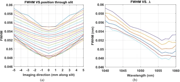
Figure 4.10 - Plot of one sampled exit slit profile (a) and resolving power across focal plane for a given grating position (b). ... 88

(14)

Figure 4.11 - Variation of FWHM as a function of position through slit (all wavelengths plotted) (a)

and wavelength (all positions through slit plotted) (b) ... 88

Figure 4.12 - Plot of one sampled exit slit profile (a) and resolution across focal plane for a given grating position (b). ... 90

Figure 4.13 - Main channel of the spectrograph with local axes of the entrance slit indicated... 91

Figure 4.14 - Alignment procedure block diagram view... 105

Figure 4.15 - Axes implementation on optical surfaces ... 106

Figure 4.16 - Toroidal lens (blue), fold mirror (grey) and detector (red) with their respective local axes ... 107

Figure 4.17 - Compensators' evolution during alignment process ... 108

Figure 4.18 – Central slit spot evolution through the different paths investigated by the algorithm .. 108

Figure 4.19 - Slit images at three different wavelengths ... 109

Figure 4.20 - Zoom onto the slit image at one detector side ... 109

Figure 4.21 - Evolution of mean spot and during alignment process ... 110

Figure 4.22 - Compensators' evolution during alignment process ... 111

Figure 4.23 - Evolution of mean spot and standard deviation during alignment process ... 111

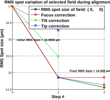
Figure 4.24 - Mean RMS spot evolution through the different paths investigated by the algorithm .. 112

Figure 4.25 - Evolution of MEAN RMS spots and standard deviation vs. focus ((a) and (b)), tilt ((c) and (d)) and tip ((e) and (f)) through focal plane at each step ... 114

Figure 4.26 – Evolution of RMS spots vs. focus ((a) and (b)), tilt ((c) and (d)) and tip ((e) and (f)) through focal plane at each step ... 115

Figure 4.27 - Induced piston at shorter and longer wavelengths after TILT movement ... 116

Figure 4.28 - Induced piston at bottom and up of the slit after TIP movement ... 117

Figure 4.29 - Resolving power through focal plane before (left) and after (right) alignment process 117 Figure 4.30 - Th-Ar spectrum [71] between 1060 and 1080 nm (a) and same part of the spectrum obtained from a U-Ne lamp [74] (b). Bottom parts of both figures are zooms from upper ones obtained when limiting the intensity y-axis. ... 119

Figure 4.31 - Calibration unit optical design. Light coming from the output end of the fiber reaches a moving fold mirror when positioned in its down position and is injected to the collimating mirror during observation (right to the fold mirror, not represented in the figure). When calibrating, the moving mirror moves upwards and light from the calibration lamps is gathered with a beamsplitter and eventually goes to the collimator. ... 120

Figure 4.32 - Detected wavelength along the slit length when taking into account the error on the repeatability of the flipping mechanism (a) and of the translation stage (b). The horizontal red line represents the mean detected wavelength and the two green ones are located at plus and minus the calibrating requirement from the exact injected wavelength... 121

Figure 4.33 - Optical design of the HCL slit illumination system ... 122

Figure 4.34 - Evolution of spectral shift with respect to scrambling gain ... 124

Figure 4.35 – Focal plane image of two central fibers (left) and profile of light intensity along imaging direction (right) with pixels ... 124

Figure 4.36 - Focal plane image of two central fibers (left) and profile of light intensity along imaging direction (right) with pixels ... 125

Figure 4.37 - Propagation of the rays from the grating zeroth diffraction order. Light is confined at the top left after hitting the walls of the calibration unit compartment and does not reach the detector. .. 126

Figure 5.1 – Star image footprint at a spectroscopic instrument’s focal plane... 131

Figure 5.2 - Bolometric correction in J-band (left: cool stars [80], right: hot stars [81] [82]) ... 132

(15)

... 134

Figure 5.5 - FRD properties and transmission of dry fibers ... 135

Figure 5.6 - Protected silver coating reflectivity ... 135

Figure 5.7 – Selected grating efficiency curve [83] ... 136

Figure 5.8 - Selected InGaAs detector quantum efficiency... 136

Figure 5.9 - Evolution of dark current (left) and quantum efficiency (right) with temperature (and wavelength) of a given cooled CCD detector ... 137

Figure 5.10 -Flux of photons received and detected for COOL stars ... 141

Figure 5.11 - Required integration time vs. for COOL stars ... 142

Figure 5.12 - Flux of photons received and detected for HOT stars ... 142

Figure 5.13 - Required integration time vs. for HOT stars ... 143

Figure 5.14 - Variation of integration time with (left: COOL stars, right: HOT stars) ... 144

Figure 5.15 - Flux of photons received and detected for COOL stars ... 145

Figure 5.16 - Required integration time vs. for COOL stars. Dashed lines in the right panel represent the saturation limit of the detector. ... 146

Figure 5.17- Optimal CCD temperature and integration time gain for COOL stars ... 146

Figure 5.18 - Evolution of integration time wrt. effective temperature for stars of magnitude 4 at different CCD temperatures (left) and integration time as a function of CCD temperature for a given cool star. ... 147

Figure 5.19 - Flux of photons received and detected for HOT stars ... 148

Figure 5.20 - Required integration time vs. for HOT stars ... 148

Figure 5.21- Optimal CCD temperature and integration time gain for HOT stars ... 149

Figure 5.22 - Evolution of integration time wrt. effective temperature for stars of magnitude 4 at different CCD temperatures (left) and integration time as a function of CCD temperature for a given HOT star. ... 149

Figure 5.23 - Variation of integration time with (left: COOL stars, right: HOT stars) ... 151

Figure 5.24 – Relationship between and (left) and evolution of required integration time as varies ... 152

Figure 5.25 – Evolution of integration time wrt. as a function of CCD temperature (left) and optimum CCD temperature as a function of . ... 153

Figure 5.26 – Relative integration time reduction by optimizing the CCD sensor temperature as a function of (left) and normalized integration time as a function of CCD temperature for low, boundary and high photon fluxes (right). ... 153

Figure 5.27 – Required integration time under better seeing conditions for cool (left) and hot stars (right). ... 154

Figure 5.28 - Required integration time with lower FRD fibers for cool (left) and hot stars (right). . 155

Figure 5.29 - Vignetting effect of fibers and instrument' collimator on integration time ... 156

Figure 5.30 – Evolution of integration time at optimal fiber core size (left) and when the collimator’s f-ration is equal to ... 156

Figure 5.31 - Required integration time when implementing micro-lenses (left: cool stars, right: hot stars) ... 157

Figure 6.1 - Fiber illuminating system ... 161

Figure 6.2 - Identification of relation between input and output fibers from the bundle ... 162

Figure 6.3 - Fiber bundle in auto-collimation with the diffraction grating. Light travels back and forth on the grating to focus at the bundle plane. ... 163

(16)

Figure 6.5 – Optical configuration that enables the alignment of the focusing mirror. The grating is positioned at the right inclination to enable the diffraction order to propagate through the system.

... 164

Figure 6.6 - Central fiber visible image through the imaging mirror ... 165

Figure 6.7 – Collimating (left) and focusing (right) mirrors ... 165

Figure 6.8 – Toroidal lens in its optical mount ... 166

Figure 6.9 – Simulated (left) and observed (right) images of the central fiber ... 166

Figure 6.10 - Full spectrograph main channel assembly ... 167

Figure 6.11 – Simulated (left) and measured (right) bundle images ... 167

Figure 6.12 - Adapted fiber illuminating system incorporating a UNe hollow cathode lamp ... 168

Figure 6.13 – Recorded spectrum of the Superlamp HCL centered at ... 169

Figure 6.14 - Recorded spectrum of a HCL by Redman et al. [74] ... 169

Figure 6.15 - Recorded spectrum of the regular HCL centered at ... 170

Figure 6.16 – Focal plane images (left) and reduced spectra (right) when observing the HCL spectrum centered at (a) , (b) and (c) ... 171

Figure 6.17 - Focal plane images (left) and reduced spectra (right) when observing the HCL spectrum centered at (a) , (b) and (c) ... 172

Figure 6.18 - Focal plane image (left) and reduced spectrum (right) when observing the HCL spectrum centered at ... 173

Figure 6.19 - Rayleigh criterion on resolving power [52] ... 173

Figure 6.20 - Reduced spectrum when observing the HCL spectrum centered at , red stars indicate spectral lines used for calibration ... 174

Figure 6.21 - Redman's atlas of a HCL centered at . Red circles indicate spectral lines used for calibration. ... 174

Figure 6.22 – Dispersion relation: the red stars are the spectral lines selected for calibration and the blue line is the order fitting. ... 175

Figure 6.23 - Calibrated spectrum when observing the HCL spectrum centered at , red stars indicate spectral lines used for calibration. ... 176

Figure 6.24 – Redman’s and calibrated recorded spectra superposed on top of each other. ... 176

Figure 6.25 - Spectral profile of the line centered at and calculation of the associated resolving power. ... 176

Figure 6.26 – Moving mirror (in home position), beamsplitter and scientific fiber (left) and mechanical slits (right). ... 177

Figure 6.27 – Superposition of both slit and bundle images. ... 178

Figure 6.28 – Profiles of bundle, spectral and flatfield slits’ images ... 179

Figure 6.29 – Hollow cathode focal plane image as seen through the bundle (a) and the mechanical slit (b). ... 179

Figure 6.30 - Spectra of the HCL as seen through the bundle (red) and the mechanical slit associated to the spectral calibration box (blue). ... 180

Figure 6.31 – Spectral profile of a given fiber (left) and detected wavelength values along with their calculated average (right). The upper and lower limits to fulfill the requirement on calibration accuracy are depicted by red dashed lines. ... 181

Figure 6.32 - Images of fibers (a), spectral calibration (b), identified lines (c), dispersion relation (d), calibrated and Redman’s spectra (e) and fiber image along with the calibrated spectrum (f). ... 182

Figure 6.33 - Horizontal component of the recorded centroids (blue circles). The mean value is indicated as a red dash-dotted line and the upper and lower limits of the tolerance interval are the red dashed lines. ... 183

(17)

Figure 7.2 – Evolution of the differential refraction as a function of wavelength at different zeniths for

two different guiding wavelengths. ... 189

Figure 7.3 - Transmission of the standard Methane filter from Custom Scientific [84]. ... 190

Figure 7.4 - Reflection of the near-infrared AR window down to the visible region [85]. ... 191

Figure 7.5 - Absolute quantum efficiency of the visible camera CCD [86]. ... 191

Figure 7.6 - Photon flux per wavelength unit for arbitrary COOL ( ) and HOT ( ) stars at - and . ... 192

Figure 7.7 – Atmospheric transmission (a), Reflectivity of the window (b), transmission of the methane filter (c) and quantum efficiency of the detector (d). ... 193

Figure 7.8 – Detected star photon flux per wavelength unit ... 194

Figure 7.9 - Integration process of the detected star photon flux per wavelength unit ... 194

Figure 7.10 - Photometric budget results ... 195

Figure 7.11 – Alignment setup of the SPS: the laser is used to illuminate the SPS optical elements ... 196

Figure 7.12 – Image of the fiber bundle onto the guiding camera. ... 196

Figure 7.13 - Complete SPS assembly with the coupling flange attached ... 197

Figure 8.1 – - , bolometric corrections and effective temperatures of identified potential targets ... 201

Figure 8.2 – Bolometric corrections of identified targets sorted according to their temperature. ... 202

Figure 8.3 - Evolution of star image size and fiber core vignetting factor as a function of seeing with the selected small telescope. Sampled values for a typical seeing of are also represented. 202 Figure 8.4 - Flux of photons received and detected at for the identified targets ... 203

Figure 8.5 - Required integration time at for the identified targets... 203

Figure 8.6 - Required integration time for the identified targets when using a CCD at the central wavelength of (left) and (right). ... 204

Figure 8.7 - Optimal CCD temperature and integration time gain for the identified targets ... 204

Figure 8.8 - Evolution of integration time as a function of different CCD temperatures for the identified targets ... 205

Figure 8.9 - Evolution of integration time wrt. as a function of CCD temperature with targets depicted on top (left) and normalized integration time as a function of CCD temperature for Betelgeuse, Spica and the boundary flux (right). ... 205

Figure 8.10 - Final configuration of the instrument with black flocked paper ... 206

Figure 8.11 - Shutters that equip the spectral calibration mechanical slit and the fiber bundle ... 207

Figure 8.12 - Fiber back-illuminating system that incorporates the LED ... 207

Figure 8.13 – Observing control room (a) and final instrument configuration with removable cover plates (b). ... 208

Figure 8.14 - Telescope initialization and remote control computer ... 208

Figure 8.15 - Flipping mirror device: the upper flange connects to the telescope, the left connecting tube intends to hold an eyepiece and the lower hidden aperture incorporates a standard thread for cameras. The small turning button activates the flipping mechanism. ... 209

Figure 8.16 - Connecting mechanical piece using the standard camera thread (a) and adapted fiber positioning system (b) ... 209

Figure 8.17 - Focal plane image when pointing at Arcturus with the initial observing setup ... 210

Figure 8.18 - Arcturus spectrum centered at from our first observation on the of June ... 211

(18)

Figure 8.19 - Advanced tracking device optical design. Light propagates from the telescope down to the bundle plane. The reflected beam onto the metallic ferrule then goes back to the beamsplitter along

with the light from the fibers and reaches the camera. ... 212

Figure 8.20 - Beamsplitter mount (a) and modified flipping mirror box (b). ... 213

Figure 8.21 – Camera holder (a) and adapted tracking device (b). ... 213

Figure 8.22 - Observation setup installed on CSL facilities roof. A second display devoted to the tracking operation was added. The laptop was dedicated to the spectrograph control. ... 214

Figure 8.23 - Internal reflections that occur within the beamsplitting glass plate. ... 214

Figure 8.24 - Simulated behavior of the ghost generation associated with the fiber bundle light (b). 215 Figure 8.25 - Multiple image formation onto the bundle ferrule due to internal reflections within the beamsplitter during the transmission process of the star light... 215

Figure 8.26 - Simulated behavior of the ghost generation issued from the star light (b). ... 216

Figure 8.27 - Focal plane image when pointing at Vega with the advanced tracking device. ... 217

Figure 8.28 - Quantum efficiency of the tracking visible camera [87]. ... 217

Figure 8.29 - Live tracking acquisition. The star image lies at the left side of the picture and the fiber bundle right above. A zoom onto the bundle enabled to tick a mark onto a fiber to lock its position after having turned off the LED. ... 218

Figure 8.30 - Focal plane image when pointing at Vega with the first update version of the advanced tracking device. ... 219

Figure 8.31 - Focal plane image when pointing at Capella with the second update version of the advanced tracking device. ... 221

Figure 8.32 - Reduced spectrum of Capella centered at after combining the different observations from the last two nights. ... 221

Figure 8.33 - NƎSIE spectrum of Capella (black solid line). The magenta spectrum corresponds to the atmospheric transmission tabulated by Hinkle et al. [93] and shifted for clarity by . The red and blue tags indicate the expected wavelengths respectively of the most prominent primary and secondary spectral features. ... 223

Figure 8.34 - Zoom on the spectral region around the triplet. The atmospheric transmission is now overplotted on the NƎSIE spectrum. The other symbols are as in Figure 8.33. . 224

(19)

(20)

List of tables

Table 1.1 - Scientific requirements on the near-infrared spectrograph ... 5

Table 1.2 - Characteristics of the TIGRE telescope ... 6

Table 1.3 - Characteristics of the ARIES telescope ... 7

Table 1.4 - Technical requirements of the MOONS instrument ... 12

Table 2.1 - Identified detectors' characteristics ... 49

Table 2.2 - Main characteristics of the Photonic Science Snake camera ... 51

Table 4.1 - The 16 parameters describing a spectrograph instrument ... 71

Table 4.2 - Spectrograph’s parameters after first and second runs ... 82

Table 4.3 - Comparison between spectrometer specifications obtained with both first resolution criterion and Bingham’s spectrometer method to obtain a resolving power of 29 000. ... 90

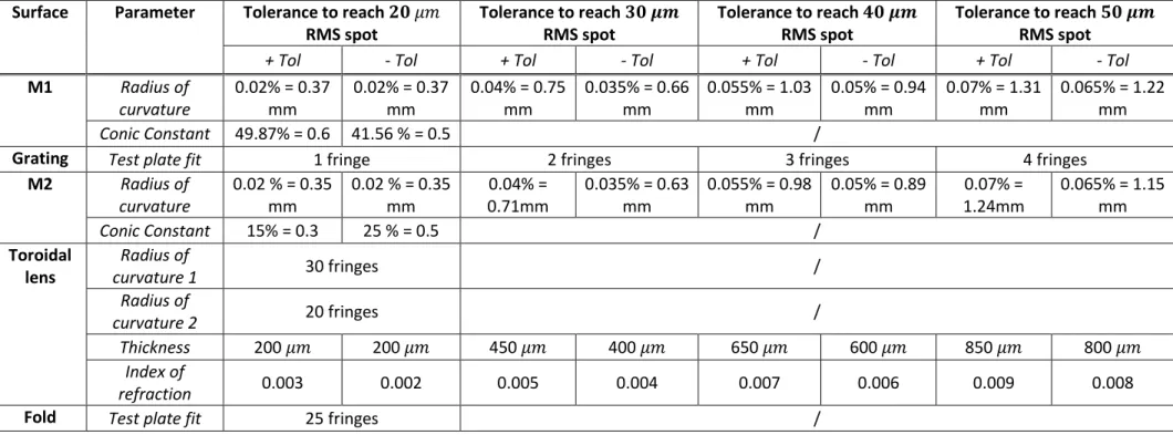
Table 4.4 – Sensitivity matrix assessing the individual effect on RMS spots of optical surfaces’ alignment ... 94

Table 4.5 - Sensitivity matrix assessing the individual effect on RMS spots of optical surfaces’ manufacturing ... 97

Table 4.6 - Typical tolerances for opto-mechanical constraints [69] ... 100

Table 4.7 - List of tolerances used when performing the overall budget of the instrument ... 102

Table 4.8 - Overall tolerancing budget results ... 103

Table 5.1 - Instrument requirements ... 129

Table 5.2 – Input parameters for the calculation of the atmospheric transmission with ATRAN ... 133

Table 5.3 - Photometric budget parameters summary ... 140

Table 5.4 - Upper wavelength limit for different - for both cool and hot stars ... 150

Table 5.5 - Transmission factors of fibers ... 155

(21)

(22)

Abstract

This research contribution intends to introduce the conception of a new fiber-fed spectrograph, called NƎSIE, that operates in the near-infrared domain. This PhD thesis was part of a research project led by Prof. Rauw which focuses on massive stars. The final location of NƎSIE will be the TIGRE telescope located in La Luz, Mexico. The observational data provided by this instrument will help several research groups from the University of Liège to study massive stars. In particularly, evolution models will be improved through the comparison of the collected spectra with theoretical models. This collaboration will therefore contribute to a better understanding of massive stars and the mechanisms that take place within these extraordinary objects.

The present manuscript will go through all the elementary steps of the design of the spectrograph: from the derivation of instrumental specifications to first light in Liège.

Key words: near-infrared spectroscopy, fiber-fed, massive stars, TIGRE telescope.

Ce travail de recherche a pour intention de présenter la conception d’un nouveau spectrographe, appelé NƎSIE, alimenté par fibres optiques qui opère dans le domaine proche-infrarouge. Cette thèse de doctorat faisait partie d’un projet de recherche mené par le Prof. Rauw centré sur les étoiles massives. La destination finale de NƎSIE sera le télescope TIGRE qui se trouve à La Luz au Mexique. Les données observationnelles fournies par cet instrument aideront plusieurs groupes de recherche de l’Université de Liège à étudier les étoiles massives. Plus particulièrement, des modèles d’évolution seront améliorés au travers de comparaisons entre les spectres collectés et les modèles théoriques. Cette collaboration contribuera dès lors à une meilleure compréhension des étoiles massives et des phénomènes qui se déroulent au sein de ces objets extraordinaires.

Le présent manuscrit parcourra l’ensemble des étapes élémentaires de la conception du spectrographe: depuis la dérivation des spécifications instrumentales jusqu’à sa première lumière à Liège.

(23)

(24)

Acknowledgement

I deeply acknowledge my co-Promoter Prof. Rauw for having offered me the opportunity to perform this PhD thesis within the frame of the ARC he supervised. The measureless amount of time he devoted me for any kind of advice, article and manuscript corrections, astrophysical and astronomical discussions was a precious help. Last but not least, I thank him for the several observations we carried out together at CSL facilities, which led to the instrument’s first light.

I gratefully thank Prof. Rochus to have trusted me and proposed me as a proper candidate for this thesis. His vast instrumental knowledge was an extensive benefit during the thesis. The guidance he ensured as a Promoter during the last four years was particularly enlightening when I faced technical issues. Continuing the spatial adventure following my Master Thesis in his company at CSL was extremely fruitful.

Thanks to my entire committee for having supervised my thesis. The association of both scientific and technical knowledge within this committee was very productive to help facing the different issues I faced during the last four years.

Thanks to my colleague, and friend, Richard Desselle for having provided some hands-on help during the last four years. Our collaboration was a mutual rewarding experience which benefited to the development of both NIR and ultraviolet innovative instrumentation for the study of massive stars.

I acknowledge the team from the University of Hamburg for their support during this project. Their practical knowledge and experience in fiber-fed spectroscopy was very helpful during this thesis. I also thank them for their technical assistance to accommodate our instrument to the TIGRE telescope.

Many thanks to all CSL people who helped during the conception and tests of this instrument. A more specific attention goes to Jérôme who involved me in the ICON project and introduced me to

(25)

Thanks to Nata for the numerous mechanical modifications he provided to the instrument enclosure. Thank you Marc to have offered me a laboratory to align and test the spectrograph. Eventually, thanks to the whole CSL staff for any involvement in my PhD thesis, from the first specifications to the first light in Liège.

Eventually, I heartily acknowledge all my family, my parents, my fiancee and my sisters without who I couldn’t have led this thesis. Their support through the entire experience, and on a broader level during all my studies, was a key factor in accomplishing this task. The hardest aspect of the thesis was probably borne by those people and I apologize for any inconvenient it may have engendered. Thanks also to my sister for the great NƎSIE logo she provided to the project. Thanks to my father for the paint work of NƎSIE’s enclosure and logo. Last but not least, thanks to my fiancee for her continuous kind presence and support particularly in the worst moments. I owe you all this successful story.

This research was funded through the ARC grant for Concerted Research Actions, financed by the Federation Wallonia-Brussels.

Ir. Christian Kintziger Faculty of Applied Sciences University of Liège (ULiège)

(26)

(27)

(28)

Introduction

Chapter 1

(29)

1. Introduction

1.1 ARC project: massive stars, key players in the evolution of the universe

he global research project that involves the present PhD thesis aims at studying massive stars. This ARC (Action de Recherche Concertée) gathers three separate research groups from the University of Liège (ULiège): the Groupe d'Astrophysique des Hautes Energies (GAPHE), the Astrophysique Stellaire Théorique et Astérosismologie (ASTA) and the Centre Spatial de Liège (CSL). The GAPHE research group is in charge of the observation of massive stars at different wavelengths. These involve the TIGRE telescope (see Chapter 1.3.1) that will host the spectrographic instrument presented throughout this manuscript. The ASTA scientific unit on the other hand focuses on theoretical simulations which aim at studying the interior of massive stars and explain their evolution process. To do so, they use among other things the asteroseismology technique. The CSL eventually covers technical aspects and within this ARC, CSL is in charge of the conception of innovative scientific instruments to study massive stars.

The main question to which the research project intends to bring some enlightening answer elements is: how do massive stars evolve? Part of the answer may reside in the mutual influences that exist between the members of binary systems. The stellar rotation must also be considered to properly assess the induced effects on the evolution processes. The existence of a magnetic field and the mass loss experienced by such stars also need to be included in the stellar evolution models. The research project therefore intends to assess all these aspects by improving the associated models and collect useful data with the developed instruments. CSL is therefore in charge of the development of new dedicated instruments to provide scientific data to the other research units. These will be used to investigate the above hypotheses and improve the numerical models. A better understanding of massive stars will therefore result from this interaction between the groups involved in the ARC.

Today’s instrumentation is largely dominated by oversubscribed telescopes which focus on a limited number of “fashionable” research topics [1]. The consequence is a lack of time for the study of massive stars, especially for long campaigns. The general actual opinion usually considers that large telescopes are better suited for spectroscopic astronomical purposes. This idea is correct when considering deep-sky observations that induce low-contrast imaging. For example, the observation of Quasars and Galaxies with small telescopes usually leads to low signal-to-noise ratio spectra and these small apertures do not actively participate to this research field [1].

The study of massive stars does not obey to this rule. Small telescopes can be used in association to low-cost instruments to conduct scientific research on stellar physics. The monitoring of the varying spectra of bright emission lines can for example be carried out with such observatories. Smaller telescopes are also naturally more numerous and easier to access than large observational platforms. This advantage therefore benefits to long-duration spectroscopic campaigns which can support other observations by larger platforms that focus on the determination of detailed spectroscopic parameters [1]. This interesting niche can therefore bring the light on poorly understood properties of massive stars and the present project intends to position our research group association as a key player in this field. This partnership intends to gather the individual expertise and give birth to a new instrument. This spectrograph will first be used on the TIGRE telescope that can be accessed by the University of Liège and is located in Mexico.

(30)

1.2 Astrophysical background

1.2.1 Massive stars

Massive stars exhibit large masses and extreme luminosities. These objects are usually the first ones we observe when targeting at galaxies [1]. However, these stars are also very rare: for one typical massive star in the Milky Way, there exist approximately a hundred thousand solar-type stars [2]. The enormous distance that separates us from the closest objects requires specific observing techniques. Indeed, standard imaging methods and even interferometric observations from combined telescopes are insufficient to provide enough resolving power. Most distance objects are therefore rather studied through spectroscopic analyses which are the key for understanding the cosmos [1]. The visibility of massive stars from large distances also enables probing the conditions of both their own environment and the intermediate space that separates us from those objects [3]. The observation of those rare objects may however be also problematic. Their visibility may indeed be threatened at early formation phases due to the surrounding dust. Some important evolution stages are also short in time and these objects usually appear in groups which complicates the understanding of evolution processes due to mutual interactions [4].

The spectroscopic analysis of bright massive stars does not require large telescopes as previously inferred. Indeed, the study of line profiles with the help of spectrographs can be performed with small telescopes when targeting massive stars. Moreover, the typical accessible time-scales for those objects range from a few minutes to several years. Their intense brightness also usually enables their observation from polluted areas close to urban centers. This benefits to amateur astronomy that can develop and supply useful complementary data to professional scientists. Long-term campaigns are usually also conducted with smaller telescopes as they are easier to access than oversubscribed large platforms.

Stars must exhibit an initial mass of approximately solar masses to be qualified as massive [3]. These “cosmic engines” highly influence their environment. Indeed, during the major part of their life, they pour to the interstellar medium high quantities of ionizing photons. On the other hand, intense and fast stellar winds are generated due to their high luminosity and irradiate their surrounding medium. Massive stars are the major source of both ultraviolet ionizing radiation in galaxies and infrared-luminosity which originates from heated dust [2]. These stars also represent the major manufacturers of carbon, nitrogen and oxygen and enrich the interstellar medium. The turbulence induced by these exchanges with their environment strongly affects the formation of stars and planets and the structure of galaxies [4].

Their death generally occurs as a gigantic supernova. This final explosion ejects several components into the neighborhood. This violent event is indeed the source of the production of newly synthesized chemical elements [3]. The black hole formation that may follow when the star collapses is the source of gamma-ray bursts which is believed by many to be the most energetic phenomenon yet found [2].

The construction of accurate models of the evolution of massive stars is therefore of high importance to properly understand all these mechanisms. Internal mixing, mass loss and binarity are three elements that still need more accurate models [3]. This accomplishment cannot be achieved without the collection of observational data to compare with theoretical information. Indeed, defects of the models can only be highlighted by observations which in turn are used to improve the numerical simulations [2].

(31)

The ARC partnership therefore intends to shed new light onto these poorly understood processes. Modeling improvements are conducted by trying to include mechanisms such as stellar rotation, mass loss, magnetic field and binarity. On the other hand, new instrumentation is under study or development by the CSL to provide observational data and compare the results with theoretical predictions.

1.2.2 The need of a near-infrared spectrograph

The full understanding of astrophysical sources requires access to a rather wide wavelength range. Every wavelength domain provides another specific piece of information that is needed to solve the puzzle. However, some wavelength domains have been somewhat neglected in recent years, despite their enormous potential. This is the case for instance of the near-IR domain around - , notwithstanding the fact that this wavelength domain can be accessed from the ground. The main reasons for this situation are the decrease in sensitivity of conventional Charge-Coupled Device (CCD) detectors in this region and the fact that most instruments are designed for longer wavelength studies, e.g. to study the ( ), ( ) and ( ) bands which are largely used in photometry.

The Near-IR (NIR) domain around has an enormous diagnostic potential for stellar activity and stellar winds, prominent features of massive stars. Indeed, these stars are very hot and luminous. Their strong UV radiation fields drive energetic and dense stellar winds that have a strong impact on the surrounding interstellar medium. In this context, the wavelength domain near is particularly interesting as it contains many spectral lines whose profiles provide useful information about stellar winds over almost the entire range of stellar masses. For example, this region contains the line, one of the few unblended lines. As it forms over almost the entire stellar wind, it has a huge diagnostic potential for models of stellar winds. Its morphology ranges from an absorption line in stars with low density winds to a broad P-Cygni profile in Wolf-Rayet stars [5] [6]. In some cases, the emission part of the P-Cygni profile is flat-topped, in other cases it is rounded or strongly peaked [7]. Whatever the morphology, it is related to the velocity law in the wind and can thus provide unique information. Moreover, this line is a good indicator of variability in the wind [7], especially for the so-called Luminous Blue Variables, which are in an intermediate evolutionary stage between and Wolf-Rayet stars where important quantities of material are lost.

Last but not least, phase-resolved observations of the line in massive binary systems are a powerful diagnostic of wind-wind interactions in these binaries [8]. But is of course not the only interesting line in this spectral domain (see Figure 1.1). Other features include , and , and lines…

On the other hand, this spectral region is also of interest for studies of the activity of low mass stars. In cool dwarf stars, chromospheric activity is a wide-spread phenomenon which manifests itself through quiescent line emission ( & , ) in the optical in addition to dramatic flaring events. Recently, it has been shown that emission in the higher order Paschen lines of hydrogen ( , , and ) as well as is a good proxy of a strong flaring activity [9] [10] [11]. Also, in the case of solar-type stars, and the Paschen lines are excellent indicators of chromospheric activity [12].

Moreover, this spectral range provides also key information on the circumstellar environment of cool giants. Indeed, in some cool giants such as Arcturus ( ), a highly variable emission

(32)

in other objects such as ( ) the line was found in absorption, but with a bluewards extension that reveals the existence of a stellar wind [14].

Finally, the line is also of major interest for the study of accretion in classical T Tauri stars. T Tauri stars are low-mass pre-main sequence stars that are still accreting material from a circumstellar disk. The emission lines observed in the spectra of these stars form at the star-disk interface or in the inner disk region. These regions have a complex topology. The high opacity of makes it a sensitive probe of both the accreting matter, in emission, and the outflowing gas via the frequently detected absorption features. Observations of this line in T Tauri stars can thus be used to constrain the wind geometry of such accreting objects [15] [16].

In summary, it is obvious that the spectral region around the line has a huge potential for many topics in stellar astrophysics. This is the reason why several research groups from Liège University have joined their forces to develop a spectrograph that covers this wavelength domain with the goal to install it at the TIGRE telescope.

Figure 1.1 - Observation of the near-IR spectrum of the Wolf-Rayet star recorded with a CCD detector. The absorption features between and are due to the Earth’s atmosphere. (Figure courtesy Jean-Marie

Vreux).

1.2.3 Scientific requirements

Scientific requirements were specified concerning the performances of the instrument under study (see Table 1.1). The conception of the spectrograph must be driven by these specifications in order to obtain an instrument which is able to do the intended science. This way, the quality of the obtained data will be high enough to tackle the scientific problems and answer open questions. Those specifications focus on spectral range, resolving power and photometric budget.

The required spectral range extends over in the near-infrared -band. The possibility to extend this latter from to is considered as a goal performance. The associated resolving power must be at least equal to but a value of is preferred. The typical observation time cannot exceed half an hour when considering target magnitudes of in -band.

Eventually, a sky measurement must be carried out to properly enable its subtraction from the data as explained further in this chapter. The wavelength calibration accuracy must also be accounted for when designing the calibration box of the instrument.

(33)

Parameter Requirement Goal Spectral range Resolving power Target magnitudes Signal-to-noise ratio in continuum at at

Typical exposure time

Simultaneous sky

measurements yes yes

Wavelength

calibration accuracy

Table 1.1 - Scientific requirements on the near-infrared spectrograph

1.3 Considered telescopes

1.3.1 el TIGRE

The TIGRE, formerly called Hamburg Robotic Telescope (HRT), is a fully robotic telescope located in La Luz, Mexico (see Figure 1.2) [17]. This private telescope is installed at an altitude of meters on a site operated by the University of Guanajuato. TIGRE is a collaboration between the universities of Hamburg (Germany), Guanajuato (Mexico) and Liège (Belgium). Currently, the only scientific instrument under operation on the TIGRE is the Heidelberg Extended Range Optical Spectrograph (HEROS), a double-channel spectrograph fed with the telescope’s light through an optical fiber. First spectroscopic light in La Luz was achieved in April and regular automatic observations from Hamburg started on August _.

The TIGRE is a Nasmyth telescope whose primary mirror has a diameter of . The typical seeing at the La Luz site amounts to on average, approaching for good nights. Therefore, this telescope is particularly well suited for the study of bright stars. Indeed, as previously noticed, this small telescope totally falls within the class of apertures that can enable intensive observations of (massive) stars.

The telescope benefits from a modern Alt-Az mount and concentrates light through a -mirror assembly to a Nasmyth focus. The spectrographic instrument that we present will be connected to the telescope through a fiber whose entrance will be placed at the currently vacant Nasmyth focus of the TIGRE telescope. The other end of this fiber will feed with light the instrument located in a separate building neighboring the telescope dome.

Figure 1.2 illustrates the TIGRE dome with the neighboring building which contains the HEROS spectrograph. Further modifications including another building are required to accommodate our NIR fiber-fed instrument. This separate room should be installed next to the HEROS enclosure and benefit from its own air conditioning system. Indeed, large temperature variations occur between day and night and this system will stabilize the instrument temperature during the day to avoid severe thermal perturbations.

(34)

Figure 1.2 - The TIGRE telescope at La Luz observatory site, Mexico [18].

The characteristics of the TIGRE telescope are summarized in the table below.

Parameter Symbol Value

Diameter

Focal length

Typical seeing

Good seeing

Table 1.2 - Characteristics of the TIGRE telescope

1.3.2 3.6M DOT (ARIES)

M DOT is a Ritchey-Chrétien telescope installed at the Devasthal Observatory site, India. Equipped with one axial port and two side ports, this telescope belongs to the Aryabhatta Research Institute of Observational Sciences (ARIES) and was first activated on March 31, 2016.

The Devasthal site is located far away from any urban development and benefits from about spectroscopic nights a year [19]. A detailed survey which lasted several years led to the careful selection of this location featuring reduced temperature variations, low relative humidity outside the rainy season and low wind speeds. Eventually, the mean observed seeing amounts to on the ground though a better value of is estimated at the telescope height [20].

The first generation focal plane instruments consist in a faint object spectrograph and camera, a high-resolution fiber-fed optical spectrograph, an optical-near infrared spectrograph and imager and a CCD optical imager [20]. On the longer term, the spectrograph we designed may be a good candidate for visiting this telescope on one of its side ports through its fiber connection. Indeed, Belgium has a guaranteed access to of the observing time on this telescope.

The versatile interface that represents the use of fibers enables to design an instrument that may be operated at several telescopes. Optical fibers facilitate this opportunity as they promote the separation of the spectrograph from the telescope focal plane. A disconnection occurs and adapting the fiber with suitable connectors enables to go from a telescope to another.

(35)

The characteristics of the ARIES telescope are summarized in the table below. The larger aperture of this telescope will benefit to the observation time. For exact photometric budget calculation, the longer focal length must also be accounted for as a larger star image may be induced depending on the local seeing.

Parameter Symbol Value

Diameter

Focal length

Typical seeing

Good seeing

Table 1.3 - Characteristics of the ARIES telescope

1.3.3 Expected seeing and image size comparison

When designing a fiber-fed instrument, a particular care to the telescope-fiber matching is required. Indeed, as much light as possible must be transmitted from the telescope to the fiber in order to minimize the required integration time. In order to collect the entire target light, the fiber core should therefore match the star image diameter, which depends on the seeing at the observation site. The typical seeing that is observed at the selected telescope location may therefore be considered in first approximation to assess the required fiber core size.

Figure 1.3 illustrates the predicted geometrical star image diameter as a function of the seeing for both identified telescopes. The observed target image size varies with the local seeing and selected telescope. Therefore, the maximum predicted star image should be considered in order to adapt to the worst observation case. However, instrumental limitations may appear due to manufacturing capabilities as will be noticed in Chapter 4.3.6. This may limit the entrance slit width of the spectrograph and the fiber core size as a direct consequence. An identified technique to overcome this issue will also be presented.

Figure 1.3 – Geometrical star image size as a function of seeing for both considered telescopes. Typical (left) and best (right) seeing conditions are also depicted.

0 0.5 1 1.5 2 0 50 100 150 200 250 300 350

Star image size in function of seeing

Seeing (arcsec) Sta r i ma ge siz e ( µ m) 93.0842 µm 172.7876 µm TIGRE ARIES 0 0.5 1 1.5 2 0 50 100 150 200 250 300 350

Star image size in function of seeing

Seeing (arcsec) Sta r i ma ge siz e ( µ m) 46.5421 µm 109.9557 µm TIGRE ARIES

(36)

1.4 Near-infrared fiber-fed spectroscopy: from pioneers to nowadays

innovators

This chapter does not intend to list the full evolution story of NIR fiber-fed spectroscopy as it cannot be exhaustive and introducing all the elementary projects is beyond the scope of this work. The technology development of fiber-fed spectrographs in general is shortly summarized in Chapter 2.4.1. Chapter 1.4.1 on the other hand intends to illustrate the first NIR fiber-fed spectrograph ever built and the associated lessons to be learnt for our own project. The evolution of the technology is illustrated with a typical instrument that is employed nowadays in Chapter 1.4.2. The comparison between the two examples will clearly highlight the achieved improvements within a few decades. Each introduced project is presented in sub-chapters depicting the individual components of the optical chain assembly. This way, every element optimization can be understood and some heritage learnt for our own spectrograph. For further examples, reference [21] establishes a rather detailed list of all multi-object fiber-fed spectrographs and projects in .

1.4.1 ISIS IR

Description

ISIS-IR is the first near-infrared fiber-fed spectrograph that was developed by Dallier et al. in the early nineties [22]. The target waveband initially included the -, - and -bands ( - .). This spectrograph was first tested at the telescope from the Pic du Midi in the south of France. Then, second tests occurred at the Mont Mégantic in Québec, Canada, with a telescope [23]. After these first assessments of the overall system performances, the spectrograph moved to the Canada-France-Hawaii Telescope (CFHT) for commissioning and observations [24].

The principal goal of this project was to mimic the already widespread visible techniques of multi-object spectroscopy to the NIR domain. Indeed, some parts of this wavelength range do not need spectrographic instruments to undergo severe modifications to properly operate in the NIR domain. The investigations of these pioneers are explained further below as they will be very useful for our own purpose.

Spectrograph

The first selected configuration for the spectrograph was the Czerny-Turner. Both the collimator and the camera were on-axis and several obstructions decreased the light transmission. These add to the one induced by the telescope because of another property of fibers: scrambling. The radial pattern of light that reaches the fiber core is mixed along the fiber length. The obstruction is thus not visible anymore at the spectrograph side of the fiber (see Chapter 2.4.2 for further explanations). The resolving power of this first setting was equal to and in - and -band respectively. The second run used other gratings and the available resolving powers were , and in -band or and in -band. The third run implemented an Ebert-Fastie configuration with resolving powers of , and in both - and -bands.

According to the authors, the selected spectral range ( to ), i.e. non-thermal IR, does not require the spectrograph to be cooled and the operation is similar to the visible waveband [22]. Only for the -band is the cooling gain important as it averages between and magnitudes [23]. On the other hand, a cold interference filter in front of the camera that matches the observed spectral band already decreases the background level. This effect is almost negligible in the - and -bands.

(37)

Fibers

The use of silica fibers for spectroscopy was already common practice and for example employed to perform multi-object spectroscopic analyses. The transmittance of these light connectors from the telescope to the spectrograph is however limited in the -band. On the other hand, - and -bands performances of dry, i.e. low content (see Chapter 2.4.2), silica fibers are perfectly acceptable [23]. Therefore, Dallier et al. first employed fluoride fibers instead because of their low spectral attenuation in the near-infrared and especially over [22]. These had never been selected for that purpose before and were successfully tested for the first time at the Pic du Midi. The observed Focal Ratio Degradation (FRD), which characterizes the widening of light beam by the fiber, was worse than the one measured with typical silica fibers. The light injection with a fast ( ) beam of light was however sufficient to minimize those losses. Since the telescope f-ratio was equal to , they used a focal reducer to adequately connect the telescope to the fiber. These fiber losses are deeply investigated in Chapter 2.4.2 but a first conclusion here is that the injection f-ratio is of major importance for the efficiency of fibers to transmit light from the telescope to the spectrograph.

The authors also pointed out that a proper light propagation occurs in a fiber when the cladding thickness equals several times the wavelength. This means packing several fibers into a bundle leads to light losses due to the absorption between the adjacent cores, especially at longer wavelengths such as the near-infrared domain. A solution already foreseen at that time was the use of a microlens array to properly sample the target flux and refocus the light only on fiber cores. The use of a fiber bundle was also seen as a suitable way for sky subtraction since the sky background is large in the -, - and -bands. Eventually, their technique to align the star image onto the fiber was a drilled metallic mirror that incorporated the fiber. The reflected light was directed to a guiding camera. Minimizing the light on the edges of the hole therefore ensured a proper transmission through the fiber.

The second observation run featured an improved fiber bundle of elements. The fibers exhibited a hexagonal pattern at the telescope side to be able to either sample the sky background with surrounding fibers around the star-dedicated one or perform small area spectroscopy [22]. Unfortunately, this second run only used a satellite fiber because two others were broken on site.

The third update of the instrument implemented regular dry silica fibers. The -band investigation was therefore limited as their transmission rapidly falls at . In any case, the high background noise due to the “warm” spectrograph configuration did not enable its use far in the -band. The hexagonal bundle packed fibers to sample the object and others to measure the surrounding sky background. As before, the bundle was reshaped at the spectrograph side to form a pseudo slit.

Detector

Another difference with the visible domain is the required use of a specific IR detector [22]. At that time, the availability of NIR cameras was growing up and enabled the development of NIR spectroscopy. As explained in Chapter 2.8.1, the early nineties correspond to an epoch where great progress was performed in the development of NIR detectors such as the NICMOS (Near Infrared Camera and Multi-Object Spectrometer) camera for the Hubble Space Telescope (HST). The first camera they used was a by CID (Charge Injection Device) cryogenic detector, a replica of the by CIRCUS camera under use at CFHT. While typical integration times of several minutes were provided by such cameras, they were initially limited to a few seconds due to an