The Relationship between Land Use Factors and Feeling of Happiness at the Neighbourhood Level



Abstract—

Happiness can be related to everything that can

provide a feeling of satisfaction or pleasure. This study tries to

consider the relationship between land use factors and feeling of

happiness at the neighbourhood level. Land use variables (beautiful

and attractive neighbourhood design, availability and quality of

shopping centres, sufficient recreational spaces and facilities, and

sufficient daily service centres) are used as independent variables and

the happiness score is used as the dependent variable in this study. In

addition to the land use variables, socio-economic factors (gender,

race, marital status, employment status, education, and income) are

also considered as independent variables. This study uses the Oxford

happiness questionnaire to estimate happiness score of more than 300

people living in six neighbourhoods. The neighbourhoods are

selected randomly from Skudai neighbourhoods in Johor, Malaysia.

The land use data were obtained by adding related questions to the

Oxford happiness questionnaire. The strength of the relationship in

this study is found using generalised linear modelling (GLM). The

findings of this research indicate that increase in happiness feeling is

correlated with an increasing income, more beautiful and attractive

neighbourhood design, sufficient shopping centres, recreational

spaces, and daily service centres. The results show that all land use

factors in this study have significant relationship with happiness but

only income, among socio-economic factors, can affect happiness

significantly. Therefore, land use factors can affect happiness in

Skudai more than socio-economic factors.

Keywords—

Neighbourhood land use, neighbourhood design,

happiness, socio-economic factors, generalised linear modelling.

I. I

OWADAYS, happiness is a goal of many national and

local governments since it could enable people to have a

better life [1]. There is a renewed interest in different areas

such as psychology, social science, and economics in

searching for happiness factors [2], [3]. Different factors such

as socio-economic (e.g. employment, inflation, and income)

and demographic factors (e.g. gender, age, marital status,

education, and health) can affect happiness [3]. Dolan et al. [4]

mentioned that all needs including income, health, and

recreational activities can affect happiness. Therefore,

happiness is the experience of satisfaction [5], and this

satisfaction can come from everything around a person [6].

M. Moeinaddini is a Senior Lecturer in Department of Urban and Regional Planning, Faculty of Built Environment, Universiti Teknologi Malaysia (corresponding author, phone: +60129410543, email: mehdi@utm.my).

Z. Asadi-Shekari is a Researcher of Universiti Teknologi Malaysia. Centre for Innovative Planning and Development (CIPD), Faculty of Built Environment, Universiti Teknologi Malaysia (e-mail: aszohreh2@live.utm.my).

Z. Sultan is a Senior Lecturer and M. Zaly Shah is an Associate Professor in Department of Urban and Regional Planning, Faculty of Built Environment, Universiti Teknologi Malaysia (email: zahids@utm.my, zaly@outlook.com).

Various studies use different factors such as quality of life,

well-being, satisfaction, and pleasure to represent happiness

[7]-[16]. Since human living settlements can affect all of the

mentioned factors, there should be a significant relationship

between the built environment and happiness [8]. For instance,

Berry and Okulicz-Kozaryn [17] proposed that levels of

development, in addition to personal characteristics, are the

key factors to happiness. One of the primary interests of some

limited studies in this area is the effect of the living place on

respondents’ happiness [18]-[22]. However, these limited

studies do not indicate which characteristics of place are most

crucial, and how components of a place that might affect

human happiness can be classified [23].

There are also some studies that consider the relationship

between happiness and environment by focusing on

macro-level factors such as air pollution, economic, and life

satisfaction at country level [24]-[26]. Welsch and Kühling

[27] focused on economics at the national level as one of the

factors that have considerable effects on the happiness level

and well-being. Dolan et al. [4] proposed that some

environmental factors at macro level such as green space, blue

space, attractive land use, air pollution, noise pollution, and

water pollution, in addition to the socio-economic factors, can

affect happiness. Hartig et al. [28] also found that attractive

landscapes can increase pleasure and happiness.

Currently, rapid urbanisation and industrialisation are the

main sources of various negative external factors such as

traffic congestions, air pollution, fossil fuel consumption,

noise pollution, and health problems [29]-[37]. These negative

external factors can affect happiness since everything around

people can affect their satisfaction level [6]. Although there is

a possible relationship between built environment and

happiness, there are limited studies that focus on this

relationship especially at neighbourhood level. Therefore, this

study focuses on this relationship by considering some land

use variables, such as beautiful and attractive neighbourhood

design, availability and quality of shopping centres, sufficient

recreational spaces and facilities, and sufficient daily service

centres (banks, educational centres, etc.), in addition to

socio-economic factors (gender, race, marital status, employment

status, education, and income), as independent variables, and

the happiness score as the dependent variable.

II. M

There are various measurement tools for happiness that

measure various happiness related indicators such as quality of

life [9], satisfaction [13], [14], well-being [4], [10], [12] and

pleasure [15], [16]. Oxford happiness questionnaire (OHQ),

M. Moeinaddini, Z. Asadi-Shekari, Z. Sultan, M. Zaly Shah

The Relationship between Land Use Factors and

Feeling of Happiness at the Neighbourhood Level

N

which was developed by Hills and Argyle [38], includes 29

items to estimate subjective well-being (SWB). The OHQ is

an improved version of the Oxford happiness inventory [39].

They improved Oxford happiness inventory (OHI) by

changing the response format. The Likert scale (1= strongly

disagree to 6 = strongly agree) was used in OHQ instead of a

0–3 multiple choice scoring format that was used in OHI. In

addition, 9 items also were added to OHI by Hills and Argyle

[38] in OHQ. Since OHQ can achieve an acceptable validity

by comparing data that were collected with other self-report

scales of SWB, this questionnaire was used in this study to

estimate the happiness score. However, more questions were

added to the mentioned questionnaire to collect some land use

data such as beautiful and attractive neighbourhood design,

availability and quality of shopping centres, enough

recreational spaces and facilities, and enough daily service

centres (banks, educational centres, etc.), in addition to the

socio-economic factors (gender, race, marital status,

employment status, education, and income). The Likert scale

was also used for land use data. The modified OHQ was used

to collect data from more than 300 people who are living in

six neighbourhoods. The neighbourhoods were selected

randomly from the main Skudai neighbourhoods in Johor,

Malaysia. Cronbach's (alpha) was used for the reliability test.

In this study, the dependent variable is the happiness score,

which comes from Likert scale response data that only takes

positive and discrete values. Therefore, conventional linear

regression models with a normally distributed error structure

are not suitable for modelling the happiness score. The GLM

framework has been more successfully adopted for this type of

data [40]-[42]. Happiness score is a scaled factor because it is

the average of Likert scale response data. Lognormal and

gamma with log link models are used to scale data in the GLM

framework [41], [42]. Exponential family models have been

more successfully adopted for the data that come from positive

and discrete values [41], [42]. Since lognormal is not in the

exponential family, GLMs with a gamma distribution are

recommended. The gamma model assumes a log link (1):

Y = EXP (β

+

∑

𝛽

× X

), (1)

where Y: dependent variable, i: subscript showing the number

of independent variables, X: independent variable, β

:

constant, calculated in the calibration process, β

coefficient of

the independent variable, calculated in the calibration process

of the model.

III. R

The results of the GLM analysis are discussed in this

section. Table I shows the reliability statistics and the

Cronbach's alpha value, which is more than 0.7. Tables II-IV,

present descriptive statistics for the variables included in the

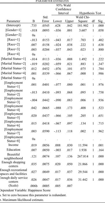
model. Table V indicates the variables included in the model,

their parameter estimates, and the significance of the

parameters (5% level). The omnibus test, likelihood ratio

square test statistics, scaled deviance (SD), and Pearson

chi-square statistic show the model goodness of fit (refer to Tables

VI and VII).

TABLEI RELIABILITY STATISTICS Cronbach's Alpha Number of Items

0.853 36

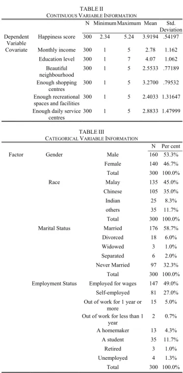
TABLEII

CONTINUOUS VARIABLE INFORMATION

N Minimum Maximum Mean Std. Deviation Dependent

Variable Happiness score 300 2.34 5.24 3.9194 .54197 Covariate Monthly income 300 1 5 2.78 1.162

Education level 300 1 7 4.07 1.062 Beautiful neighbourhood 300 1 5 2.5533 .77189 Enough shopping centres 300 1 5 3.2700 .79532 Enough recreational

spaces and facilities

300 1 5 2.4033 1.31647 Enough daily service

centres

300 1 5 2.8833 1.47999

TABLEIII

CATEGORICAL VARIABLE INFORMATION

N Per cent

Factor Gender Male 160 53.3%

Female 140 46.7% Total 300 100.0% Race Malay 135 45.0% Chinese 105 35.0% Indian 25 8.3% others 35 11.7% Total 300 100.0% Marital Status Married 176 58.7% Divorced 18 6.0%

Widowed 3 1.0%

Separated 6 2.0% Never Married 97 32.3%

Total 300 100.0% Employment Status Employed for wages 147 49.0% Self-employed 81 27.0% Out of work for 1 year or

more

15 5.0% Out of work for less than 1

year 2 0.7% A homemaker 13 4.3% A student 35 11.7% Retired 3 1.0% Unemployed 4 1.3% Total 300 100.0% TABLEIV

CASE PROCESSING SUMMARY N Per cent

Included 300 100.0%

Excluded 0 0.0%

Total 300 100.0%

Table VIII indicates that there is no strong correlation

between the independent variables included in the model since

tolerances are greater than 0.1 and the VIFs are less than 10.

Therefore, the final model can be defined as:

HS = EXP (0.735 + 0.019I + 0.121B + 0.035S + 0.027R +

0.026DS), (2)

where HS = happiness score, I = income, B = beautiful

neighbourhood, S = sufficient shopping centres, R = sufficient

recreational spaces and facilities, DS = sufficient daily service

centres.

Interval Hypothesis Test Lower Upper Wald Chi-Square df Sig. (Intercept) .735 .0545 .628 .842 181.902 1 .000 [Gender=1] -.018 .0093 -.036 .001 3.607 1 .058 [Gender=2] 0a . . . . [Race=1] -.013 .0153 -.043 .017 .703 1 .402 [Race=2] .007 .0158 -.024 .038 .222 1 .638 [Race=3] .003 .0204 -.037 .043 .023 1 .880 [Race=4] 0a . . . . [Marital Status=1] -.014 .0113 -.036 .008 1.492 1 .222 [Marital Status=2] -.019 .0202 -.059 .021 .883 1 .347 [Marital Status=3] .012 .0452 -.076 .101 .075 1 .784 [Marital Status=4] .001 .0339 -.066 .067 .000 1 .986 [Marital Status=5] 0a . . . . [Employment Status=1] .001 .0401 -.077 .080 .001 1 .976 [Employment Status=2] -.013 .0410 -.093 .068 .095 1 .758 [Employment Status=3] -.004 .0442 -.090 .083 .006 1 .936 [Employment Status=4] .042 .0665 -.088 .173 .408 1 .523 [Employment Status=5] .020 .0437 -.066 .105 .205 1 .651 [Employment Status=6] .015 .0418 -.067 .097 .134 1 .715 [Employment Status=7] .003 .0590 -.113 .118 .002 1 .962 [Employment Status=8] 0a . . . . Income .019 .0056 .008 .030 11.594 1 .001 Education .007 .0050 -.003 .017 1.938 1 .164 Beautiful neighborhood .121 .0074 .107 .136 267.814 1 .000 Enough shopping centers .035 .0075 .020 .050 21.866 1 .000 Enough recreational

spaces and facilities .027 .0049 .017 .037 29.544 1 .000 Enough daily service

centers .026 .0047 .017 .036 31.442 1 .000 (Scale) .006b .0005 .005 .007

Dependent Variable: Happiness Score

a. Set to zero because this parameter is redundant. b. Maximum likelihood estimate.

This model shows that happiness is significantly affected by

land use and neighbourhood design factors. Among these

indicators, beautiful neighbourhood has higher positive

parameters; therefore, this indicator has greater effects on

happiness in this model. The second effective indicator with a

positive relationship is enough shopping centres. Income is the

only significant socio-economic indicator. Overall, more

beautiful neighbourhoods and enough shopping centres,

recreational spaces and facilities, and daily service centres, in

addition to higher income, could contribute to more happiness.

TABLEVI OMNIBUS TEST

Likelihood Ratio Chi-Square df Sig.

367.934 21 .000

Dependent Variable: Happiness Score

Model: (Intercept), Gender, Race, Marital Status, Employment Status, Income, Education, Beautiful neighbourhood, Enough shopping centres, Enough recreational spaces and facilities, Enough daily service centres

Compares the fitted model against the intercept-only model. TABLEVII

SD AND PEARSON CHI-SQUARE GOODNESS OF FIT

Value df Value/df

Deviance 1.699 278 .006

Scaled Deviance 300.283 278

Pearson Chi-Square 1.640 278 .006 Scaled Pearson Chi-Square 289.989 278

Dependent Variable: Happiness Score

Model: (Intercept), Gender, Race, Marital Status, Employment Status, Income, Education, Beautiful neighbourhood, Enough shopping centres, Enough recreational spaces and facilities, Enough daily service centres

TABLEVIII COLLINEARITY STATISTICS

Tolerance VIF

Income .970 1.030

Enough daily service centers .430 2.328 Enough recreational spaces and facilities .460 2.172 Enough shopping centers .564 1.773 Beautiful neighborhood .656 1.525

IV. D

C

The relation between land use factors and happiness has not

received enough attention to date. Previous happiness studies

were overwhelmingly focused on socio-economic as well as

demographic factors but only recently scholars across many

disciplines have begun to explore the question of happiness

and life satisfaction. Previous studies have identified the

positive relationship between income and happiness [43]-[48].

Although the present study also endorses this significant

relationship, it failed to find significant association between

other socio-economic factors such as gender, marital status,

education level, and employment status with happiness.

Therefore, the results of the present study are unique and

interesting from the perspective of land use factors that are

significant in the proposed model.

Some of the previous studies proposed a positive

relationship between education level and SWB or happiness

[49], [50]. There are a number of studies from the perspective

of low income countries, which show that education has a

positive relationship with happiness [51], [52]. However, the

present study is in line with Flouri [53], which proposed no

significant relationship between education level and

happiness. Employment status is another key variable which

has been discussed widely in the literature. Although previous

studies consistently show a large negative effect of individual

unemployment on happiness [54]-[56], the present study does

not find any significant relationship between employment

status and happiness since the present study does not focus on

individual unemployment and the proportion of unemployed

people is not considerable (1.3%) in this study (refer to Table

III).

The present study identifies more significant role for land

use factors statistically. It implies that beautiful

neighbourhoods and nearby recreational as well as shopping

facilities make the people happier. For example, enough

recreational facilities at neighbourhood is one of land use

variables that have a positive significant relationship with

happiness. This association is in line with previous studies

which proposed that even simple types of exercise such as

gardening [57] may be associated with higher life satisfaction

and happiness that is especially important for people over 60

years [58].

3Mixed land use planning at neighbourhood level may

increase the social activities and increase time for leisure.

According to Haworth [59], leisure and happiness are

interrelated. An individual may use leisure as an opportunity

to cope with work stress [60]. Attractive and beautiful

neighbourhood design may produce positive moods, and much

of this derived pleasure stems from the social relationships

that they foster [39]. The results are in line with previous

studies [61]-[64], which identified that social activities and

frequency of participation in leisure activities are associated

positively with happiness [65]. Neighbourhood design

indicators are extensively addressed in literature from

sustainability perspective but there is less focus on land use

factors from the perspective of resident’s feeling of happiness.

Our cities, particularly in developing countries, fail to make

the residents happy. Some design changes at neighbourhood

level may improve the happiness scale of residents.

A

The authors wish to thank all of those who have supported

this research for their useful comments during its completion.

In particular, we would like to acknowledge the Universiti

Teknologi Malaysia Research Management Centre (RMC) and

Centre for Innovative Planning and Development (CIPD).

This research received funding from the Ministry of

Education, Malaysia under the Fundamental Research Grant

Scheme (FRGS) 2015 (FRGS grant no:R.J130000.7821.

4F739).

R

[1] Helliwell, J. F., Layard, R., Sachs, J. (2015). Setting the Stage. In J. F. Helliwell, R. Layard, J. Sachs (Eds.), World Happiness Report 2015. New York City, US: Columbia University.

[2] Tokuda, Y., Inoguchi, T. (2008). Interpersonal mistrust and unhappiness among Japanese people. Social Indicators Research, 89, 349-360. [3] Andrés Rodríguez-Pose, A., Von Berlepsch, V. (2012). Social Capital

and Individual Happiness in Europe. Bruges European Economic Research Papers: Department of European Economic Studies.

[4] Dolan, P., Peasgood, T., White, M. (2008). Do we really know what makes us happy? A review of the economic literature on the factors associated with subjective well-being, Journal of Economic Psychology 29, 94–122.

[5] Radwan, M.F. (2014). The Psychology of Attraction Explained: Understand what attracts people to each other. Create Space: Independent Publishing Platform.

[6] Ferreira, S. Moro, M. (2010). On the use of subjective well-being data for environmental valuation. Environmental and Resource Economics, 46(3), 249–273.

[7] Savageau, D. (2007). Places rated Almanac. Washington, DC: Places Rated Books LLC.

[8] Ballas, D., Dorling, D. (2013). The geography of happiness. In S. David, I. Boniwell, A. Conley Ayers (Eds.), The Oxford handbook of happiness. Oxford, UK: Oxford University Press.

[9] Marans, R.W., Stimson, R.J. (2011). An Overview of Quality of Urban Life in R.W. Marans, R.J. Stimson (Eds.), Investigating quality of urban life: Theory, Methods, and Empirical Research. New York City, US: Springer.

[10] Gowdy, J. (2005). Toward a new welfare economics for sustainability. Ecological Economics, 53(2), 211–222.

[11] Dolan, P., Peasgood, T., White, M. (2008). Do we really know what makes us happy? A review of the economic literature on the factors associated with subjective well-being, Journal of Economic Psychology 29, 94–122.

[12] Welsch, H. Kühling, J. (2009). Using happiness data for environmental valuation: Issues and applications. Journal of Economic Surveys, 23, 385-406

[13] MacKerron, G. Mourato, S. (2009). Life satisfaction and air quality in London. Ecological Economics, 68, 1441–1453.

[14] Menz, T., Welsch, H., (2010). Population aging and environmental in OECD countries: The case of air pollution. Ecological Economics, 69(12), 2582–2589.

[15] Maddison, D. Rehdanz, K. (2011). The impact of climate on life satisfaction. Ecological Economics, 70, 2437-2445.

[16] Raphael, D., Renwick, R., Brown, I., Steinmetz, B., Sehdev, H. Phillips, S. (2001). Making the links between community structure and individual well-being: Community quality of life in Riverdale, Toronto, Canada. Health and Place, 7, 179-196.

[17] Berry, B., Okulicz-Kozaryn, A. (2009). Dissatisfaction with City Life: A New Look at Some Old Questions. Cities, 26, 117-124.

[18] Booth M. Z., Sheehan, H. C. (2008). Perceptions of people and place: Young adolescents’ interpretation of their schools in the United States and the United Kingdom. Journal of Adolescent Research, 23(6), 722-744.

[19] Cramer, V., Torgersen, S., Kringlen, E. (2003). Quality of life in a city: The effects of population density. Social Indicators Research, 69, 103-116.

[20] Delken, E. (2008). Happiness in shrinking cities in Germany. Journal of Happiness Studies, 9, 213-218.

[21] Scoppa, V., Ponzo, M. (2008). An empirical study of happiness in Italy. The Berkeley Electronic Journal of Economic Analysis and Policy, 8(1), 1-21.

[22] Solano, A. C., Morales, J. F. D. (2002). Life goals and life satisfaction in Spanish and Argentine adolescents from rural and urban settings. Psicothema, 14(1), 112-117.

[23] Morrison, P. (2007). Subjective wellbeing and the city. Social Policy Journal of New Zealand, 31, 74-103.

[24] Ballas, D., Dorling, D. (2007). Measuring the impact of major life events upon happiness. International Journal of Epidemiology, 36, 1244–1252. [25] Marshall, A. Jivraj, S. Nazroo, J. Tampubolon, G. Vanhoutte, B. (2014).

Does the level of wealth inequality within an area influence the prevalence of depression amongst older people? Health and Place 27, 194–204.

[26] Menz, T. (2011). Do people habituate to air pollution? Evidence from international life satisfaction data. Ecological Economics, 71, 211-219. [27] Welsch, H. Kühling, J. (2009). Using happiness data for environmental

valuation: Issues and applications. Journal of Economic Surveys, 23, 385-406

[28] Hartig, T., Van Den Berg, A., Hagerhall, C. M., Tomalak, M., Bauer, N., Hansmann, R., Ojala, A., Syngollitou, E., Carrus, G., van Herzele, A., Bell, S., Podesta, M. T. C., Waseth, G. (2010). Health benefits of nature experience: Psychological, social and cultural processes. In K. Nilsson, M. Sangster, C. Gallis, T. Hartig, S. de Vries, K. Seeland, J. Schipperijn (Eds.), Forests, Trees and Human Health. New York City, US: Springer.

[29] Moeinaddini, M., Asadi-Shekari, Z., Ismail, C. R., Zaly Shah, M. (2013). A Practical Method for Evaluating Parking Area Level of Service. Land Use Policy, 33, 1-10.

[30] Moeinaddini, M., Asadi-Shekari, Z., Zaly Shah, M. (2014b). Analyzing the Relationship between Park-and-Ride Facilities and Private Motorized Trips Indicators. Arabian Journal for Science and Engineering, 39(5), 3481-3488.

[31] Moeinaddini, M., Asadi-Shekari, Z., Zaly Shah, M. (2015b). An Urban Mobility Index for Evaluating and Reducing Private Motorized Trips. Measurement, 63, 30-40.

[32] Asadi-Shekari, Z., Moeinaddini, M., Zaly Shah, M. (2013a). Disabled pedestrian level of service method for evaluating and promoting inclusive walking facilities on urban streets. Journal of Transportation Engineering, 139, 181–192.

[33] Asadi-Shekari, Z., Moeinaddini, M., Zaly Shah, M. (2013b). Non-motorised Level of Service: Addressing Challenges in Pedestrian and Bicycle Level of Service. Transport Reviews, 33, 166–194.

[34] Asadi-Shekari, Z., Moeinaddini, M., Zaly Shah, M.(2014). A pedestrian level of service method for evaluating and promoting walking facilities on campus streets. Land Use Policy, 38, 175-193.

[35] Asadi-Shekari, Z., Moeinaddini, M., Zaly Shah, M. (2015a) A Bicycle Safety Index for Evaluating Urban Street Facilities. Traffic Injury Prevention, 16, 283-288.

[36] Asadi-Shekari, Z., Moeinaddini, M., Zaly Shah, M. (2015b). Pedestrian Safety Index for Evaluating Street Facilities in Urban Areas. Safety Science, 74, 1-14.

[37] Asadi-Shekari, Z., Moeinaddini, M., Sultan, Z., Zaly Shah, M., Hamzah, A. (2015c). The Relationship between Street Network Morphology and Percentage of Daily Trips on Foot and by Bicycle at the City-Level. JurnalTeknologi, 76 (14), 23-28.

[38] Hills, P., Argyle, M. (2002). The Oxford Happiness Questionnaire: a compact scale for the measurement of psychological well-being. Personality and Individual Differences, 33, 1073–1082.

[39] Hills, P., Argyle, M. (1998). Positive moods derived from leisure and their relationship to happiness and personality. Personality and Individual Differences, 25 (3), 523-535.

[40] Hadayeghi, A. (2009). Use of Advanced Techniques to Estimate Zonal Level Safety Planning Models and Examine Their Temporal Transferability. Toronto, Canada: University of Toronto (Doctor of Philosophy).

[41] Moeinaddini, M., Asadi-Shekari, Z., Zaly Shah, M. (2014a). The Relationship between Urban Street Networks and the Number of Transport Fatalities at the City Level. Safety Science, 62, 114-120. [42] Moeinaddini, M., Asadi-Shekari, Z., Sultan, Z., Zaly Shah, M. (2015a).

Analyzing the Relationships between the Number of Deaths in Road Accidents and the Work Travel Mode Choice at the City Level. Safety Science, 72, 249–254.

[43] Frey, B. S., Stutzer, A. (2002). Happiness and economics. Princeton, US: Princeton University Press.

[44] Clark, A., Frijters, P., Shields, M. (2008). Relative income, happiness, and utility: An explanation for the Easterlin paradox and other puzzles. Journal of Economic Literature, 46(1), 95- 144.

[45] Ahuvia, A. C. (2007). Wealth, consumption and happiness. In A. Lewis (Ed.), The Cambridge handbook of psychology and economic behaviour. Cambridge, UK: Cambridge University Press.

[46] Ahuvia, A. C., Friedman, D. (1998). Income, consumption, and subjective well-being: Toward a composite macromarketing model. Journal of Macromarketing, 18, 153–168.

[47] Diener, E., Biswas-Diener, R. (2002). Will money increase subjective well-being? A literature review and guide to needed research. Social Indicators Research, 57, 119–169.

[48] Layard, R. (2005). Happiness: Lessons form a new science. London, UK: Penguin Press.

[49] Blanchflower, D. G., Oswald, A. J. (2004). Well-being over time in Britain and the USA. Journal of Public Economics, 88, 1359–1386. [50] Stutzer, A. (2004). The role of income aspirations in individual

happiness. Journal of Economic Behaviour and Organisation, 54, 89– 109.

[51] Fahey, T., Smyth, E. (2004). Do subjective indicators measure welfare? Evidence from 33 European societies. European Societies, 6(1), 5–27. [52] Ferrer-i-Carbonell, A. (2005). Income and well-being: An empirical

analysis of the comparison income effect. Journal of Public Economics, 89, 997–1019.

[53] Flouri, E. (2004). Subjective well-being in midlife: The role of involvement of and closeness to parents in childhood. Journal of

Happiness Studies, 5, 335-358.

[54] Di Tella, R., MacCulloch, R., Oswald, A. (2001). Preferences over inflation and unemployment. Evidence from surveys of happiness. The American Economic Review, 91(1), 335–341.

[55] Frey, B. S., Stutzer, A. (2000). Happiness, economy and institutions. The Economic Journal, 110, 918–938.

[56] Helliwell, J. F. (2003). How’s life? Combining individual and national variables to explain subjective well-being. Economic Modelling, 20, 331–360.

[57] Ferrer-i-Carbonell, A., Gowdy, J. M. (2007). Environmental degradation and happiness. Ecological Economics, 60(3), 509–516.

[58] Baker, L. A., Cahalin, L. P., Gerst, K., Burr, J. A. (2005). Productive activities and subjective well-being among older adults: The influence of number of activities and time commitment. Social Indicators Research, 73, 431–458.

[59] Haworth, J. T. (1997). Work, leisure and well-being. London/New York: Routledge.

[60] Trenberth, L., Dewe, P., Walkey, F. (1999). Leisure and its role as a strategy for coping with work stress. International Journal of Stress Management, 6 (2), 89-103.

[61] Ragheb, M. G. (1993). Leisure and perceived wellness: A field investigation. Leisure Sciences, 75 (1), 13-24.

[62] Dowall, J., Bolter, C., Flett, R., Kammann, R. (1988). Psychological well-being and its relationship to fitness and activity levels. Journal of Human Movement Studies, 14 (1), 39-45.

[63] Lloyd, K., Auld, C. J. (2002). The role of leisure in determining quality of life: Issues of content and measurement. Social Indicators Research, 57 (1), 43-71.

[64] Wankel, L., Berger, B. (1990). The psychological and social benefits of sport and physical activity. Journal of Leisure Research, 22 (2), 167-182. [65] Baldwin, K., Tinsley, H. (1988).An investigation of the validity of Tinsley and Tinsley’s (1986) theory of leisure experience. Journal of Counseling Psychology, 35 (3), 263-267.