Pépite | Décomposition des gains de productivités et distribution des effets prix entre les parties prenantes

Texte intégral

(1)Thèse de Karina Shitikova, Université de Lille, 2018. Equation Chapter 1 Section 1. Université de Lille LEM - Lille Economie Management - UMR 9221 IÉSEG School of Management ED SESAM-Sciences Economiques, Sociales, de l’Aménagement et du Management. Productivity gains decomposition and distribution of the price effects among stakeholders Thèse en vue de l’obtention du titre de Docteur en Sciences Economiques. Karina Shitikova 2 juillet 2018 ____________________________________________________________ Membres du Jury Rapporteurs: Vivian Valdmanis, Professor, Western Michigan University, USA Yves Surry, Professor, Swedish University of Agricultural Sciences, Uppsala, Sweden Examinateurs : Raluca Parvulescu, Professeure Assistant, IÉSEG School of Management Olivier de La Villarmois, Professeur des Universités, IAE Paris, Université Paris Panthéon Sorbonne Directeurs : Hervé Leleu, Directeur de Recherche CNRS, LEM UMR 9221 Jean-Philippe Boussemart, Professeur des Universités, Université de Lille, LEM UMR CNRS 9221. © 2018 Tous droits réservés.. lilliad.univ-lille.fr.

(2) Thèse de Karina Shitikova, Université de Lille, 2018. L’Université de Lille n’entend donner aucune approbation ni improbation aux opinions émises dans cette thèse. Ces opinions doivent être considérées comme propres à leur auteur.. LABORATOIRE DE RATTACHEMENT : Lille Économie Management (LEM – UMR CNRS 9221), Laboratoire de recherche rattaché au CNRS, à l’Université de Lille et à la Fédération Universitaire Polytechnique de Lille (FUPL) Préparation de la thèse au LEM sur le site de l’IÉSEG School of Management, 3 Rue de la Digue, 59000 Lille. 2 © 2018 Tous droits réservés.. lilliad.univ-lille.fr.

(3) Thèse de Karina Shitikova, Université de Lille, 2018. Acknowledgements. First, I would like to express my great acknowledgement to my supervisors Jean-Philippe Boussemart and Hervé Leleu for giving me the opportunity to undertake this PhD program. During all these years your expertise, patience, availability helped me a lot to advance through this challenging journey. Thanks for sharing with me your knowledge and experience, for giving me valuable advice and suggestions. I would like to thank IESEG School of Management for providing me with excellent conditions to realize my PhD. I would like especially to thank its director, Jean-Philippe Ammeux, for hosting me at this institution through all my PhD and accepting me as a Teaching and Research Assistant. I am also grateful to l’Université Catholique de Lille for giving me the financial support that allowed me to perform my research project. I am also acknowledged to LEM laboratory for providing me with financial resources to go to the conferences. I thank as well my university of inscription, l’Université de Lille and l’Ecole Doctorale SESAM. My special thanks go to Raluca Parvulescu, my colleague from the Economics department with who I had a chance to collaborate. Our discussions, your advice and support encouraged me a lot in difficult moments throughout this process. I would like also to thank Albane Tarnaud with who I shared the office for more than two years. Thanks for helping me to integrate this school, for your support and availability. I am also grateful to Maia Gejadze for giving me some precious suggestions that made me advance significantly. I cannot forget all my PhD colleagues (or already doctors) that made this journey more exciting: Cristina Ciobanu, Jenny Tran, Kristine Tamayo, Helen Cocco, Adrian Barragan Diaz, Minh Phan, Arno de Caigny, Khoi Pham, Annabelle Glaize, Marion Lauwers, Hélène Stefaniutyn, Salim Rostami, Zhiyang Shen, Libo Li, Steven Debaere, Stijn Geuens. Finally, I would like to thank my parents and my sister for ongoing help and moral support during all these years.. 3 © 2018 Tous droits réservés.. lilliad.univ-lille.fr.

(4) Thèse de Karina Shitikova, Université de Lille, 2018. General abstract. The financial performance of a firm depends both on its productive efficiency and the economic environment in which this firm performs its activity. Several seminal works studied the relationship between financial performance and productivity and the way the productivity gains are distributed among the beneficiaries. This thesis adds to the literature by developing new links between productive efficiency, financial performance and productivity gains distribution. Namely, this doctoral thesis contributes in the three following ways. First, we propose an original way on how to decompose the profit gaps among firms at the crosssectional level taking into account their productive inefficiency and then relating these productivity-based gaps to the price advantages/disadvantages of the firm’s stakeholders. This methodological framework was applied to a sample of US banks over the period 2001-2012. The analysis was focused on the banks with positive profit gap over the whole period and before and after the crisis. The results showed that over the considered period performant banks benefitted from positive price environment but were inefficient in their productivity levels. The main providers of financial resources for performant banks were creditors and employees over the entire period and suppliers after the 2007-2008 financial crisis. Besides, a decrease in allocative inefficiency is observed after the crisis. Finally, a comparison analysis of commercial and savings banks revealed that the main source of price advantages was creditors for the former and suppliers for the latter over the whole period. Second, we define an indicator of price environment for a firm comparing its distance to the volume- and value-based efficiency frontier. These price environment effects were computed for US industries from 1987 to 2014. The groups of industries with similar price effects evolutions were found and a panel model was performed to determine the influence of each stakeholder price effect on the global price effect. The results indicated that global mean price environment for all sectors was deteriorating over the entire period which can be related to the increasing degree of openness of US economy. This analysis showed that all specific input/output effects were statistically significant. A strong influence could be observed for capital, gross output and labor price environments. Intermediate inputs affected global price environment much less. Besides, structural breaks occurred in the beginning of 2000s and around 2005-2007 (the financial crisis).. 4 © 2018 Tous droits réservés.. lilliad.univ-lille.fr.

(5) Thèse de Karina Shitikova, Université de Lille, 2018. Third, we suggest a decomposition of the overall technical inefficiency of firms at the aggregated level into two components: individual technical and individual structural inefficiencies. This decomposition was applied to the same data as for the second analysis. The convergence process was studied for both components and a panel procedure was used to link the two components changes to the changes of the stakeholder’s price advantages/disadvantages. The results clearly confirm the convergence processes for both technological catching-up and input-output mixes. Using the link existing between TFP growth rate and price advantages/disadvantages, we then estimate the influence of technical and structural inefficiency changes on each stakeholder’s compensation. A panel data regression revealed that customers and managers benefitted substantially from the two convergence processes while the opposite was found for suppliers. Employees and capital providers seemed not to be affected by technical inefficiency and inputoutput mixes convergence processes since their price changes seem essentially driven by the macro business cycle. This essay tends to show that generation of productivity gains and their distribution are two sides of the same coin. The former is related to the economic analysis of TFP based on the estimation of a production technology while the latter deals with an accounting approach of business performance. By considering that firms should not only to be studied from the production side but also from their trading relationships, we contribute to build the bridge between economists and managers in the evaluation of business performances.. Keyword : Total Factor Productivity ; Productivity Accounting ; Price Advantages ; Data Envelopment. Analysis ;. Banks ;. U.S.. Industries ;. Technical/Structural. Inefficiencies ;. Technological Catching-up.. 5 © 2018 Tous droits réservés.. lilliad.univ-lille.fr.

(6) Thèse de Karina Shitikova, Université de Lille, 2018. Résumé général Décomposition des gains de productivités et distribution des effets prix entre les parties prenantes La performance financière d'une firme dépend à la fois de son efficacité productive et de l'environnement économique dans lequel cette firme exerce son activité. Quelques contributions importantes ont étudié la relation entre la performance financière et la productivité et la manière dont les gains de productivité sont répartis entre les bénéficiaires. Cette thèse enrichit cette littérature en développant de nouveaux liens entre l’efficacité productive, la performance financière et la distribution des gains de productivité. Trois contributions principales y sont développées. Premièrement, nous proposons une manière originale de décomposer les écarts de profit entre les firmes au niveau spatial en tenant compte de leur inefficacité productive et en reliant ensuite ces écarts aux avantages/désavantages prix des parties prenantes de la firme. Ce cadre méthodologique a ensuite été appliqué à un échantillon de banques américaines sur la période 2001-2012. Les résultats ont montré que tout au long de la période considérée, les banques les plus performantes ont bénéficié d'un environnement de prix positif mais montraient des niveaux de productivité inférieurs. La source des avantages prix pour les banques proviennent essentiellement de leurs clients créditeurs et de leurs employés sur toute la période et de leurs fournisseurs après la crise financière de 2007-2008. En outre, une diminution de l'inefficacité allocative est observée après la crise. Enfin, une analyse comparative entre les banques commerciales et les caisses d'épargne a révélé que la principale source d'avantages prix était les prêteurs pour les premiers et les fournisseurs pour les seconds sur l'ensemble de la période. Deuxièmement, nous définissons, d’un point de vue méthodologique, un indicateur de l'environnement prix pour une firme en comparant sa distance à la frontière d'efficacité estimée, d’une part, avec des volumes et, d’autre part, avec des valeurs. Cet effet d'environnement prix a été ensuite appliqué pour l’ensemble des industries américaines sur la période 1987-2014. Des groupes d'industries ayant des évolutions d’effets prix similaires ont été mis en évidence et un modèle de données de panel a été estimé pour déterminer l'influence de l’effet prix associé à chaque partie prenante sur l’effet prix global. Les résultats ont indiqué que l'environnement prix global moyen pour tous les secteurs se détériorait sur l’ensemble de la période, ce qui peut être lié au niveau d'ouverture croissant de l'économie américaine à la concurrence internationale. Cette analyse a aussi montré que tous les effets spécifiques à chaque input/output étaient statistiquement 6 © 2018 Tous droits réservés.. lilliad.univ-lille.fr.

(7) Thèse de Karina Shitikova, Université de Lille, 2018. significatifs. Une forte contribution du capital, de la production et du travail sur l’effet prix globale a pu être observée. Les inputs intermédiaires ont beaucoup moins affecté l'environnement prix global. En outre, deux ruptures structurelles se sont produites au début des années 2000 et autour de 2005-2007 précédant juste la crise financière. Troisièmement, nous développons une approche méthodologique pour décomposer l'inefficience technique globale des firmes à un niveau agrégé tel que le secteur ou l’économie en deux composantes : l’inefficacité technique individuelle et l’inefficacité structurelle. Cette décomposition a été appliquée aux mêmes données américaines que pour la deuxième analyse. Un processus de convergence a été étudié pour les deux composantes et une analyse de données de panel a été utilisée pour lier les changements des deux composantes aux changements des avantages/désavantages prix des parties prenantes. Les résultats confirment clairement les processus de convergence à la fois pour le rattrapage technologique et pour les processus de production (mix d’input/output). En utilisant le lien existant entre le taux de croissance de la productivité globale des facteurs (PGF) et les avantages/ désavantages prix, nous estimons ensuite l'influence des changements d'inefficiences technique et structurelle sur la rémunération de chaque partie prenante. Une régression en données de panel a révélé que les clients et les managers ont bénéficié substantiellement des deux processus de convergence alors que le contraire a été trouvé pour les fournisseurs. Les employés et les fournisseurs de capitaux n’ont pas été affectés par les processus de convergence de l'inefficacité technique et des processus de production car leurs avantages prix semblent essentiellement être reliés aux cycles macroéconomiques. Au final, ce travail de thèse tend à montrer que la génération des gains de productivité et leur distribution entre les parties prenantes d’une firme sont les deux facettes d'une même pièce. La première est liée à l'analyse économique de la PGF basée sur l'estimation d'une technologie de production tandis que la seconde traite d'une approche comptable et managériale de la performance des firmes. En considérant que les firmes ne doivent pas seulement être étudiées du côté de la production mais aussi du point de vue des leurs échanges, nous contribuons à établir un pont entre les économistes et les gestionnaires dans l'évaluation des performances des firmes. Mots clés : Productivité Globale des Facteurs ; Comptes de Surplus ; Avantages Prix ; Data Envelopment Analysis ; Banques ; Industries Américaines ; Inefficacité Technique/Structurelle ; Rattrapage Technologique.. 7 © 2018 Tous droits réservés.. lilliad.univ-lille.fr.

(8) Thèse de Karina Shitikova, Université de Lille, 2018. Résumé substantiel. Le profit est habituellement considéré comme un indicateur privilégié de la performance économique d’une firme et la maximisation du profit est souvent utilisée comme l'hypothèse de base du comportement du producteur dans la théorie néoclassique. Mais, derrière cet indicateur de rentabilité globale, beaucoup d'autres sont aussi essentiels tels que les efficacités technique (utiliser les ressources de manière optimale), allocative (allouer efficacement les ressources en fonction de leur prix respectif), d’échelle (produire à la taille optimale), productive (maximiser la productivité), coût (minimiser les coûts) ou revenu (maximiser le revenu). En considérant tous ces concepts de performance productive, les décisions managériales sont prises et concernent l’ensemble des facteurs de production comme le travail, les équipements, les consommations intermédiaires, les actifs financiers... Même si la croissance de la productivité impacte fortement la rentabilité, celle-ci ne dépend pas uniquement de la performance productive. Elle est également influencée par l'environnement prix dans lequel une firme opère. Un environnement prix très avantageux peut conduire à des résultats financiers positifs, même sans efficacité productive. L'inverse est également possible : une firme efficace au niveau productif peut souffrir d'un environnement prix désavantageux. Au final, c’est à la fois la performance productive et l'environnement prix qui contribuent à la rentabilité. D’un autre côté, la rentabilité d'une entreprise a une influence sur les échanges financiers avec ses parties prenantes : prêteurs, employés, propriétaires, clients et fournisseurs. Par conséquent, la performance d’une firme doit être analysée à travers deux dimensions principales, à savoir la production et les échanges. En effet, mesurer la performance productive n'est qu'un aspect de l'image globale. L'autre face concerne la répartition des gains de productivité entre les parties prenantes qui contribuent à l'activité de l'entreprise. Dans cette thèse, nous avons développé de nouvelles façons de lier la productivité, la performance financière et l'environnement prix. Plus précisément, ce travail propose trois études sur la décomposition des gains de productivité et la répartition des effets prix entre les parties prenantes. Ces travaux sont tous basés sur une approche commune qui est l’estimation non paramétrique d’une technologie de production et développée dans le premier chapitre. Une première contribution de notre se situe dans le deuxième chapitre qui introduit une nouvelle décomposition de la différence de profit entre deux firmes et relie celle-ci à la définition des comptes de surplus. La seconde contribution est développée dans le troisième chapitre qui présente la définition d’un indicateur d'environnement prix global pour les firmes. Il est basé sur une comparaison de 8 © 2018 Tous droits réservés.. lilliad.univ-lille.fr.

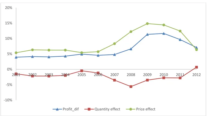
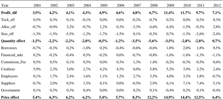
(9) Thèse de Karina Shitikova, Université de Lille, 2018. l’efficience des firmes à partir de données en quantité et en prix et permet de définir un indicateur global mais aussi des indicateurs d’environnement prix spécifiques à chaque input/output et que nous pouvons directement reliés aux parties prenantes. Dans le quatrième et dernier chapitre, nous proposons une décomposition originale de l'inefficience technique agrégée au niveau sectoriel en deux composantes et relie leurs changements dans le temps aux changements des avantages prix des parties prenantes. Dans ce qui suit, nous présentons en quelques lignes des principales contributions et résultats des chapitres deux à quatre. Le chapitre 2 décompose l’écart de profit mesuré entre deux firmes en trois effets « quantité » (inefficience technique, inefficacité allocative et effet taille) et un effet « prix » global ensuite réparti en avantages prix spécifique à chacune des parties prenantes. Au final, nous montrons comment le surplus de productivité qui est la somme effets quantités est distribué entre les parties prenantes à travers leurs avantages/désavantages prix respectifs, y compris le profit qui est la rémunération du propriétaire de la firme. En comparaison avec l'approche habituelle du CERC (Centre d’Etude des Revenus et des Coûts), l'originalité de notre travail réside dans le fait que les variations de profit sont étudiées dans une dimension spatiale plutôt que temporelle. L’objet de l’analyse est davantage orienté vers la comparaison des profits entre firmes plutôt que l’analyse de la variation du profit d’une firme dans le temps. Une autre spécificité de notre travail est que nous utilisons systématiquement les indicateurs de Bennet pour tous les effets quantité et prix. Cette méthodologie permet d'identifier à la fois les effets des différences d'efficacité technique, d'allocation des ressources et de taille ainsi que l'effet de différents environnements prix sur l'écart de profit entre deux entreprises. De plus, du point de vue des comptes de surplus, elle permet de déterminer les sources du surplus de productivité qui sont ensuite réparties entre les parties prenantes. Ce cadre a été appliqué à un échantillon de banques américaines sur la période 20012012. Nous avons réalisé notre analyse en termes de différences de taux de profit plutôt que de niveau de profit pour maitriser l’effet taille. Nous avons restreint notre analyse aux seules banques « performantes » qui montraient en moyenne un écart de taux de profit positif par rapport à l’ensemble des autres banques. Les résultats ont montré que tout au long de la période considérée, les banques les plus performantes ont bénéficié d'un environnement de prix positif mais montraient des niveaux de productivité inférieurs. La source des avantages prix pour les banques proviennent essentiellement de leurs clients créditeurs et de leurs employés sur toute la période et de leurs fournisseurs après la crise financière de 2007-2008. En outre, une diminution de l'inefficacité allocative est observée après la crise. Enfin, une analyse comparative entre les banques commerciales et les caisses d'épargne a révélé que la principale source d'avantages prix était les prêteurs pour les premiers et les fournisseurs pour les seconds sur l'ensemble de la période. 9 © 2018 Tous droits réservés.. lilliad.univ-lille.fr.

(10) Thèse de Karina Shitikova, Université de Lille, 2018. Dans le chapitre 3, nous définissons, d’un point de vue méthodologique, un indicateur de l'environnement prix pour une firme en comparant sa distance à la frontière d'efficacité estimée, d’une part, avec des volumes et, d’autre part, avec des valeurs. La comparaison des distances à ces deux frontières conduit à définir un indicateur d'environnement prix en considérant à la fois les quantités et les prix comme des variables de décision. Cette méthodologie peut être utilisée pour une mesure globale de l'environnement prix mais aussi appliquée pour définir un environnement prix spécifique à chaque input et output. Cet effet d'environnement prix a été ensuite appliqué pour l’ensemble des industries américaines sur la période 1987-2014. Des groupes d'industries ayant des évolutions d’effets prix similaires ont été mis en évidence et un modèle de données de panel a été estimé pour déterminer l'influence de l’effet prix associé à chaque partie prenante sur l’effet prix global. Les résultats ont indiqué que l'environnement prix global moyen pour tous les secteurs se détériorait sur l’ensemble de la période, ce qui peut être lié au niveau d'ouverture croissant de l'économie américaine à la concurrence internationale. Cette analyse a aussi montré que tous les effets spécifiques à chaque input/output étaient statistiquement significatifs. Une forte contribution du capital, de la production et du travail sur l’effet prix globale a pu être observée. Les inputs intermédiaires ont beaucoup moins affecté l'environnement prix global. En outre, deux ruptures structurelles se sont produites au début des années 2000 et autour de 2005-2007 précédant juste la crise financière. Dans le dernier et quatrième chapitre, nous développons une approche méthodologique pour décomposer l'inefficience technique globale des firmes à un niveau agrégé tel que le secteur ou l’économie en deux composantes : l’inefficacité technique individuelle et l’inefficacité structurelle. Cette décomposition a été appliquée aux mêmes données américaines que pour la deuxième analyse. Un processus de convergence a été étudié pour les deux composantes et une analyse de données de panel a été utilisée pour lier les changements des deux composantes aux changements des avantages/désavantages prix des parties prenantes. Les résultats confirment clairement les processus de convergence à la fois pour le rattrapage technologique et pour les processus de production (mix d’input/output). En utilisant le lien existant entre le taux de croissance de la productivité globale des facteurs (PGF) et les avantages/ désavantages prix, nous estimons ensuite l'influence des changements d'inefficiences technique et structurelle sur la rémunération de chaque partie prenante. Une régression en données de panel a révélé que les clients et les managers ont bénéficié substantiellement des deux processus de convergence alors que le contraire a été trouvé pour les fournisseurs. Les employés et les fournisseurs de capitaux n’ont pas été affectés par les processus de convergence de l'inefficacité technique et des processus. 10 © 2018 Tous droits réservés.. lilliad.univ-lille.fr.

(11) Thèse de Karina Shitikova, Université de Lille, 2018. de production car leurs avantages prix semblent essentiellement être reliés aux cycles macroéconomiques. Au final, ce travail de thèse tend à montrer que la génération des gains de productivité et leur distribution entre les parties prenantes d’une firme sont les deux facettes d'une même pièce. La première est liée à l'analyse économique de la PGF basée sur l'estimation d'une technologie de production tandis que la seconde traite d'une approche comptable et managériale de la performance des firmes. Les principales contributions de ce travail ont été d'abord de relier ces deux aspects d'un point de vue méthodologique, et puis de montrer l'utilité de cette analyse conjointe en termes d'effets quantité et prix pour des applications au monde réel. Grâce à ce cadre analytique, nous sommes désormais capables d'aller au-delà de la simple mesure de l'efficacité productive en reliant ses composantes technique, allocative et de taille aux avantages des parties prenantes. En considérant que les firmes ne doivent pas seulement être étudiées du côté de la production mais aussi du point de vue des leurs échanges, nous contribuons à établir un pont entre les économistes et les gestionnaires dans l'évaluation des performances des firmes.. 11 © 2018 Tous droits réservés.. lilliad.univ-lille.fr.

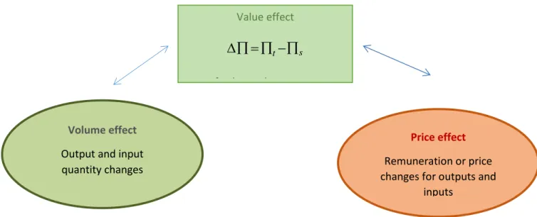
(12) Thèse de Karina Shitikova, Université de Lille, 2018. Table of contents. Acknowledgements. 3. General Abstract. 4. Résumé général. 6. Résumé substantiel. 8. Table of contents. 12. General Introduction. 15. Chapter 1 Efficiency, productivity accounting and profit decomposition. 20. 1 Introduction. 20. 2 Efficiency and productivity. 21. 2.1 Production technologies. 21. 2.1.1 Definition of production sets based on quantities. 21. 2.1.2 Definition of the distance function: an equivalent representation of the production set 28 2.1.3 Measures of productive, technical and scale efficiencies. 30. 2.1.4 Measures of economic efficiency: cost, revenue, profit and allocative efficiency 32 2.2 Estimations of distance function. 35. 2.2.1 Non parametric estimation by Data Envelopment Analysis. 36. 2.2.2 A numerical example. 40. 3 Generation and distribution of productivity gains over time 3.1 Surplus Account. 45 45. 3.1.1 Introduction to surplus account. 45. 3.1.2 Objective. 46. 3.1.3 Splitting the created value into volume and price effect. 47. 3.2 Productivity Surplus and TFP. 49. 3.3 Empirical illustration. 53. 3.3.1 Data. 53. 3.3.2 The total productivity surplus computed with a Laspeyres approach. 55. 3.3.3 The surplus account. 56. 3.4 A real world application: the U.S. automobile industry and the U.S. economy 3.4.1 The productivity gains over 1987-2014. 59 59. 12 © 2018 Tous droits réservés.. lilliad.univ-lille.fr.

(13) Thèse de Karina Shitikova, Université de Lille, 2018. 3.4.2 Losers and winners in the repartition of the productivity gains. 60. 3.4.3 Conclusion. 62. 4 Quantity and price effects in profit differential between two firms. 63. 4.1 Decomposition of the profit differential between two firms. 63. 4.2 Technical, Allocative and Size efficiency effects. 64. 4.2.1 Notations. 65. 4.2.2 Decomposition of the quantity effect. 66. 4.3 Distribution of efficiency gains among stakeholders. 67. 4.4 Explaining the profit rate differential between banks. 69. References. 70. Chapter 2 A case study on U.S. banks industry. 73. 1 Introduction. 73. 2 A brief review of the banking sector in the U.S.. 74. 3 An application to US banks over 2001-2012. 75. 3.1 Data and the underlying technology. 75. 3.2 Results and analysis. 81. 3.2.1 A detailed analysis for two banks: The Lorain National Bank and Northrim Bank 82 3.2.2 A global analysis for performant banks. 86. 3.2.3 An analysis of performant banks before and after the financial crisis. 89. 3.2.3.1 A cluster analysis of performant banks before and after crisis. 95. 3.2.3.2 Explaining clusters by a canonical discriminant analysis. 97. 4 Conclusion. 104. References. 105. Chapter 3 Measuring the effects of price environment: An application to U.S. industries 106 1 Introduction. 106. 2 Methodology. 108. 3 Empirical analysis: data and results. 113. 3.1. Data. 113. 3.2. Results. 113. 3.2.1 Total price environment for the U.S. economy. 113. 13 © 2018 Tous droits réservés.. lilliad.univ-lille.fr.

(14) Thèse de Karina Shitikova, Université de Lille, 2018. 3.2.2 A cluster analysis of the industries’ total price environments. 116. 3.2.3 The decomposition of the total price environment into individual output and input price effects. 125. 4 Conclusions. 129. References. 130. Chapter 4 Technological catching-up and growth convergence among U.S. industries 132 1 Introduction. 132. 2 Analyzing convergence process with directional distance functions. 136. 2.1. Definition and measure of a technical catching-up process. 136. 2.2. Definition and measure of a structural convergence process. 139. 3. Data and results. 143. 3.1. Data. 144. 3.2. Technical catching-up and structural convergence processes among U.S. industries 144. 3.3. The linkage between stakeholder’s price advantages and convergence processes 149. 3.3.1. Definition of price advantages. 149. 3.3.2. Price advantages and TFP growth. 150. 3.3.3. The model linking price advantages and technical and structural inefficiency scores 152. 4 Conclusion. 154. References. 155. General conclusion. 158. Appendix 1 Chapter 1 Implementation in SAS of the numerical example from section 2.2.2 161 Appendix 2 Chapter 2 SAS codes to compute technically efficient and profit maximizing benchmarks. 164. Appendix 3 Chapter 2 Profit rate gap evolution and its decomposition into quantity and price effects for a sample of 35 US banks presented over at least 2004-2012. 171. Appendix 4 Chapter 2 Canonical discriminant analysis. 176. 14 © 2018 Tous droits réservés.. lilliad.univ-lille.fr.

(15) Thèse de Karina Shitikova, Université de Lille, 2018. General introduction. Profit is usually considered as the economic performance indicator and the profit maximization is often used as the assumption of a producer behavior in neoclassical theory. But behind this global profitability indicator, many other factors are underlying such as technical, allocative, scale, scope, cost or revenue efficiencies. Underlying all these concepts of productive performance, management decisions are made concerning the best allocation of resources such as employees, equipment, intermediate inputs, and financial assets. While productivity growth strongly impacts profitability, the latter does not only depend on productive performance. It is also influenced by price environment in which a firm operates. A very advantageous price environment can lead to positive financial results even without productive efficiency. The inverse is also possible: a productively efficient firm can suffer from a disadvantageous price environment. Finally, both productive performance and price environment contribute to the profitability. Moreover, profitability of a firm has a financial influence on its stakeholders: lenders, employees, owners, customers and suppliers. Consequently, firm performance should be analyzed through two main dimensions namely production and transaction. Indeed measuring productive performance is only one side of the global picture. The other part concerns the distribution of productivity improvements among the stakeholders who contribute to the firm activity. From a more global perspective, Davis (1947, 1955) noticed that economic progress not only depends on productivity growth but also on the distribution of the productivity gains among all participants of society. Kendrick (1961) and, Kendrick and Sato (1963) initiated studies on analyzing generation and distribution of Total Factor Productivity (TFP) growth by combining price and quantity changes simultaneously. Their results show that productivity changes can be gauged either from quantity changes or from price variations. Nevertheless, most of studies succeeding these pioneering works rest at a macro or sectoral level (Hulten et al., 2001). However, this concern is considered as a key issue in performance analysis at the micro level. Davis (1947, 1955) and Kendrick (1961) also studied the relationship between productivity changes and individual financial performance by linking quantity, price and profitability variations. In this way, they explored the distribution of the returns of productivity growth among the different participants contributing to the firm’ activities. Davis (1947, 1955) attributed a monetary value to productivity change and shared it between six major stakeholders while 15 © 2018 Tous droits réservés.. lilliad.univ-lille.fr.

(16) Thèse de Karina Shitikova, Université de Lille, 2018. Kendrick (1961) explored the distribution of productivity gains among clients, suppliers, company owners and government at a durable manufacturing corporation. More precisely in the case of productivity growth, the consumers possibly will get benefit from price decreases or higher quality products, employees could earn greater compensation, intermediate input providers may receive higher prices, stockholders may obtain greater dividends, companies themselves could improve retained earnings and finally, the government may benefit from higher taxes. In the same vein, a large number of studies underlining the connection between generation and distribution of productivity gains was developed by a group of French economists. Initiated by Vincent (1968) and precisely settled through the document edited by the Centre d’Etudes des revenus et des Coûts (CERC, 1980), the methodology was applied to analyze the performances of several French public firms such as Electricité de France (EDF), Gaz de France (GDF), les Charbonnages de France and Société Nationale des Chemins de Fer Français (SNCF). More recently, TFP analysis has known a significant revival with innovative researches (Fried et al., 2008). More particularly, greater attention has been focused on the distribution of the gains from TFP through price effect components at the firm level. Following this way, Grifell-Tatjé and Lovell (2015) studied the link between productivity and financial performance indicators, the sources of productivity growth and the way the benefits of productivity growth are distributed and quantify a complete analytical framework within each of these aspects. They refer to the models and extensions treating the relation between productivity and profitability and the way the fruits of the productivity growth are distributed among the beneficiaries developed by Davis (1955), Kendrick and Creamer (1961), Vincent (1968) and CERC (Centre d’Etudes des Revenus et des Coûts) institution (1980). They underline that a larger amount of information can be extracted by economists from financial accounts to analyze business performance. This research takes place in the literature on productivity gains decomposition and distribution of the price effects among stakeholders establishing the formal link between productivity change and profitability. The thesis is based on three main contributions developed throughout four chapters. First, we start with the decomposition of profit differences into quantity and price effects. Traditionally a multiplicative decomposition is made in the time dimension where profit change among two periods for a specific firm is analyzed. In our work, we are more interested in the spatial dimension and a new and original additive decomposition of profit differences is proposed at the cross-sectional level. In this framework, the quantity effect of the profit decomposition 16 © 2018 Tous droits réservés.. lilliad.univ-lille.fr.

(17) Thèse de Karina Shitikova, Université de Lille, 2018. reveals productivity gaps among firms which can be assimilated to the concept of productivity surplus (PS) as introduced by the CERC (1980). PS is further decomposed into three effects related to the sources of productive inefficiency namely technical, allocative and size effects. Then PS is equated to the sum of price advantages (PA) associated with each stakeholder and computed as the price differences among firms. In that perspective, the first chapter is devoted to methodological aspects of production theory, modelling production technologies through distance functions, defining productivity and efficiency measures and estimating them by a nonparametric DEA framework. In addition, methodological aspects of surplus accounts are covered to analyze generation and distribution of productivity gains among stakeholders. Numerical examples and study cases are systematically developed to show the operational implementation of these concepts and tools for managers and practitioners. By integrating this two strands of literature, we finally propose a methodological contribution to decompose profit differential between two firms into quantity and price effects. Based on this contribution, chapter two offers a real-world application on U.S. small and medium banks over the period from 2001 to 2012. Price advantages of each stakeholder (creditors, employees, suppliers, government, borrowers, financial market participants and, commission and fee payers) are decomposed and analyzed. Finally, we compared surplus productivity accounts for banks with positive profit rate gap between the two periods before and after the 2007-2008 crisis. Second, we develop a new methodology for estimating the impact of price environment on firm performance. Starting with a traditional definition of a production technology as developed by Shephard (1953, 1970), Koopmans (1951), Debreu (1951) and Farrell (1957), we extend the Data Envelopment Analysis (DEA) framework to introduce a value efficiency measure which is compared to the technical efficiency to define a price environment indicator. The latter distinguishes itself from the usual allocative efficiency since it does not require resource reallocation at the firm level. It is based on a comparison of prices among peers. In chapter three, we propose a price environment indicator for a Decision-Making Unit (DMU) taking into account the quantity-price correspondences. Two technologies are defined: one formed with observed quantities and the other constituted with observed values. Efficiency scores under these two technologies are estimated and then ratios of value efficiency scores to volume efficiency scores are computed. Obtained ratios are interpreted as indicators of positive or negative price environment for a DMU. We employ Shephard’s output distance function to retrieve technical efficiency scores under both value and quantity technologies. Such indicators can be implemented for measuring the global price environment taking into account all output and input prices 17 © 2018 Tous droits réservés.. lilliad.univ-lille.fr.

(18) Thèse de Karina Shitikova, Université de Lille, 2018. simultaneously or for estimating specific output or input price effects. This methodology is applied to all 63 U.S. industries over the period 1987-2014. Third, we investigate the sources of price advantage changes for stakeholders related to productivity catching up. We separate efficiency gaps into two components: a technical efficiency effect taking into account size heterogeneity and a structural component which highlights the impacts of an input-output deepening or expanding effect on technological transfer over time. This original decomposition serves as the basis of the final chapter in which the technical catching-up and the convergence of input-output mixes among the US industries over 1987-2014 is analyzed. After demonstrating the equality between TFP growth rate and the sum of weighted price advantages, we propose a panel data analysis to estimate the influence of technical and structural inefficiency variations on the price advantages changes for each stakeholder (clients, suppliers, employees, capital providers and managers). An application analyzes input-output ratio convergence and technical efficiency catching-up among 63 North American industries over the period 1987-2014.. References CERC, (1980), Productivité globale et compte de surplus, documents du Centre d’Etude des Revenus et des Coûts, La documentation française, n°55/56, 218 p. Davis, H.S., (1947), The Industrial Study of Economic Progress, Philadelphia, University of Pennsylvania Press. Davis, H.S., (1955), Productivity Accounting, Philadelphia, University of Pennsylvania Press. Debreu, G., (1951), The Coefficient of Resource Utilization, Econometrica, 19(3), 273-292. Farrell, M. J., (1957), The Measurement of Productive Efficiency, Journal of the Royal Statistical Society, 120(3), 253-290. Fried, H., Lovell, C.A.K., Schmidt, S.S., eds., (2008), The Measurement of Productive Efficiency and Productivity Growth, New York: Oxford University Press. Grifell-Tatjé, E., Lovell, C.A.K., (2015), Productivity Accounting, The Economics of Business Performance, Cambridge University Press, 386 p. Hulten, C.R., Dean, E., Harper, M.J., Conference on Research in Income and Wealth, (2001), New developments in productivity analysis, Studies in income and wealth, 63, Chicago, Ill., Univ. of Chicago Press, 631p.. 18 © 2018 Tous droits réservés.. lilliad.univ-lille.fr.

(19) Thèse de Karina Shitikova, Université de Lille, 2018. Kendrick, J.W., (1961), Productivity Trends in the United States, Princeton, NJ: Princeton University Press. Kendrick, J.W., Creamer, D., (1961), Measuring Company Productivity: Handbook with Case Studies, Studies in Business Economics, 74, New York: The Conference Board. Kendrick, J.W., Sato, R., (1963), Factor Prices, Productivity, and Economic Growth, The American Economic Review, 53(5), 974-1003. Koopmans, T. C., (1951a), Analysis of Production as an Efficient Combination of activities, Activity Analysis of Production and Allocation, Chapter 13, 33-37, New York, Wiley. Koopmans, T. C., (1951b), Efficient Allocation of Resources, Econometrica, 19(4), 455-465. Shephard, R. W., (1953), Cost and Production Functions, Princeton, New Jersey, Princeton University Press. Shephard, R.W., (1970), Theory of cost and production functions, No. 4, in Gale, D., Kuhn, H. W., (Eds.), Princeton, New Jersey, Princeton University Press. Vincent, A.L.A., (1968), La Mesure de la Productivité, Paris: Dunod.. 19 © 2018 Tous droits réservés.. lilliad.univ-lille.fr.

(20) Thèse de Karina Shitikova, Université de Lille, 2018. Chapter 1 Efficiency, productivity accounting and profit decomposition. 1 Introduction In this chapter we present the methodological settings used in chapters 2, 3 and 4. In the first part of the second section, we focus on efficiency and productivity measures and on how these measures can be estimated. For this, we follow the literature developed by Shephard (1953, 1970), Koopmans (1951) and Debreu (1951). First, we introduce the definition of a production possibility set based on the underlying assumptions. Second, we define the distance function as the measurement tool over production sets providing an equivalent representation of the technology. Based on this approach, a nonparametric estimator (Data Envelopment Analysis, DEA) of the distance function is presented in the second part of the second section. DEA constructs an efficient frontier based on a sample of observed Decision Making Units (DMUs) and estimates inefficiency scores. In this chapter, only nonparametric deterministic framework is considered, other possibilities of estimating distance functions are stated but not developed. In the third section, we develop the theory behind the surplus accounting method. First, it gives a general idea of the methodology and its objective and then presents the Productivity Surplus (PS) estimation itself. It provides the classical CERC’s approach (CERC, 1980) with Laspeyres-and Paasche based surplus accounts for both PS and Price Advantages (PA) related to the different stakeholders participating in the production process. Then, this methodology is extended to the Bennet productivity and price advantage indicators. Furthermore, an explicit link between Total Factor Productivity (TFP) changes and PS is established. A numerical example illustrates a practical implementation of the CERC productivity methodology. Finally, a real data application analyzes and compares productivity gains evolution and their distribution over time between US automobile sector and the whole US economy. In the fourth section, we propose a new methodology to decompose a profit gap between two firms in quantity and price effects through a Bennet approach. Then, three components of the quantity effect are identified namely technical, allocative and size indicators. As to the price effect, it is decomposed among stakeholders and the link to surplus accounting is established. Finally, we introduce a ratio instead of the usual additive decomposition for this methodology in order to solve the commensurability issue of profit comparisons between firms. 20 © 2018 Tous droits réservés.. lilliad.univ-lille.fr.

(21) Thèse de Karina Shitikova, Université de Lille, 2018. 2 Efficiency and productivity 2.1 Production technologies The seminal works of Koopmans (1951), Debreu (1951), Shephard (1953), and Farrell (1957) have developed the basis of the Neo-Walrasian production theory based on production sets. To define a basic production technology, we assume that decision making units (DMUs) have N number of inputs (x) that can be used to produce M number of outputs (y). Understanding theoretical production principles behind productive reality are crucial to model production functions. 2.1.1 Definition of production sets based on quantities General definitions We can consider a technology as a process of transformation of a number of inputs into a number of outputs. We suppose that this process is an unknown model (black box) for economists and we only know that specific outputs can be produced using specific inputs. Examples of technology can be: agriculture (use of yields, fertilizers, irrigation, mechanization, pesticides and animal feed to produce meat, milk, eggs and cereals); health (use of hospitals, facilities, equipment, expertise, people and materials to produce goods and services in healthcare system); finance (use of customer deposits, employees, structures and equipment to produce loans, marketable securities and investments and services). The classical production possibility set (or technology) can be defined as follows:. T (x,y)  RN  M : x can produce y. (1). It can be illustrated as in Figure 1 where one input x is used to produce one output y. T(x,y) represents the set of all feasible production plans. The boundary of this set gives the maximum output that can be produced for each level of input. It can be understood as the best practices and it is usually named as the efficient frontier. Production plans inside the set are feasible but not efficient.. 21 © 2018 Tous droits réservés.. lilliad.univ-lille.fr.

(22) Thèse de Karina Shitikova, Université de Lille, 2018. Figure 1 Production possibility set In case of multiple outputs and/or multiple inputs, the production technology can also be represented by an output and/or an input correspondence. The output set is defined by all possible output combinations that can be produced by a given level of inputs. The output correspondence is defined as:. P(x)  y  RM : (x, y) T . (2). Figure 2 Output correspondence Figure 2 illustrates the output set P(x) when two outputs (y1 and y2) can be produced from a vector of inputs (x). Feasible output combinations are inside P(x) and the boundary defines the efficient frontier. Similarly, the production technology can be characterized by an input set, namely all possible input combinations that can produce a given level of outputs. The input correspondence is defined as: 22 © 2018 Tous droits réservés.. lilliad.univ-lille.fr.

(23) Thèse de Karina Shitikova, Université de Lille, 2018. L(y) x  RN : (x,y) T . (3). An illustration of input sets is given in Figure 3.. Figure 3 Input correspondence A key theoretical result is that both output correspondence (P(x)) and input correspondence (L(y)) are equivalent representation to the production possibility set (T(x,y)). Therefore, economists can work on one or another representation which is the most appropriate to the context. Axioms The definition of a production technology given so far is general and only determines a global analysis frame for a certain number of inputs that can be transformed into outputs using the specific technology. To give more structure to a considering set and, especially, to ensure the reliability of the modelling of the transformation of inputs into outputs, a certain number of axioms need to be defined. They are intended to give an economic sense to input-output sets. They are often called in economics “regularity conditions”. A first axiom asserts that no productions can be made without using any resources. It is called the « No free lunch » axiom and can be expressed as follows:. If (x, y) T and x  0, then y  0. (4). Axiom of free disposability of inputs and outputs is the capacity to stock, eliminate and waste factors and productions. Formally, free disposability is defined as follows for inputs: 23 © 2018 Tous droits réservés.. lilliad.univ-lille.fr.

(24) Thèse de Karina Shitikova, Université de Lille, 2018. If (x, y) T and (x', y)  (x, y) then (x', y)  T. (5). The equation (5) specifies that if it is possible to produce a certain amount of outputs (y) using a given amount of inputs (x), then we hypothesize that a firm will be able to produce the same amount of output using more inputs (x’). This definition does not consider the case of congestion as when the excessive use of inputs can affect negatively the production of outputs. Following the same logic, the free disposability of outputs can be presented as follows:. If (x, y) T and (x, y')  (x, y) then (x, y') T. (6). The expression (6) underlines that if a firm produces a certain amount of outputs using a given amount of inputs, it can also produce less using the same amount of inputs. Otherwise speaking, the waste of outputs is allowed. A free disposability of outputs can be interpreted in Figure 4. Y2. III. III. Free disposability. P(x) Y1 0. Figure 4 Free disposability of outputs The convexity axiom allows us to distinguish two types of technologies: DEA technology which supposes convexity of production set and FDH (Free Disposal Hull) that does not suppose convexity. If only two dimensions are considered, one can define easily if the set is convex: it is impossible to link any two points of a convex set with a line not completely included in the set. To define the convexity in more than two dimensions, one needs to consider a more general definition. A set is convex if all the combinations of vectors belonging to the set also belong to the set. This axiom can be expressed as: 24 © 2018 Tous droits réservés.. lilliad.univ-lille.fr.

(25) Thèse de Karina Shitikova, Université de Lille, 2018. If (xk , y k )  T , k  1,..., K , then  k (xk , y k )  T with k  0 k and k. . k. 1. (7). k. A convex production frontier is displayed in Figure 5. Y. T(x,y) is convex set. X. 0. Figure 5 Convexity An alternative to convex sets is proposed by Deprins et al. (1984) as Free Disposal Hull (FDH). The FDH set is non-convex and can be figured in Figure 6. The frontier of the FDH set has a staircase. shape.. FDH. is. only. based. on. the. free. disposability. assumption.. Y. III. III. T(x,y) is non-convex set. X 0. Figure 6 Free Disposal Hull Moreover, the axiom of returns to scale implies the rate of change in outputs to inputs. Constant returns to scale (CRS) assume that all outputs are expended or reduced by a proportional increase or decrease in all inputs. Non-increasing returns to scale (NIRS) show outputs are scaled less than or equal to inputs. Non-decreasing returns to scale (NDRS) indicate outputs are scaled more than or equal to inputs. If none of these cases hold, the technology is characterized by variable returns 25 © 2018 Tous droits réservés.. lilliad.univ-lille.fr.

(26) Thèse de Karina Shitikova, Université de Lille, 2018. to scale (VRS). The demonstrations of CRS, NIRS, NDRS, and VRS are presented in Figures 7, 8, 9 and 10 respectively. The first theoretical developments in DEA, namely the model of Charnes, Cooper et Rhodes (CCR, Charnes et al. (1978)) are based on CRS hypothesis. It can be formulated as follows:. If (x,y) T and   0, then (x, y) T Y. X 0. Figure 7 Constant returns to scale Non-increasing returns to scale (NIRS) suppose:. If (x,y) T and 0    1, then (x, y) T Y. X 0. Figure 8 Non-increasing returns to scale The mathematical expression for non-decreasing returns to scale (NDRS) is the following: 26 © 2018 Tous droits réservés.. lilliad.univ-lille.fr.

(27) Thèse de Karina Shitikova, Université de Lille, 2018. If (x,y) T and   1, then (x, y) T Y. X 0. Figure 9 Non-decreasing returns to scale Variable returns to scale (VRS) were introduced by Banker, Charnes et Cooper (1984) and hold when none of the previous models are valid.. Y. X 0. Figure 10 Variable returns to scale. 27 © 2018 Tous droits réservés.. lilliad.univ-lille.fr.

(28) Thèse de Karina Shitikova, Université de Lille, 2018. 2.1.2 Definition of the distance function: an equivalent representation of the production set The axioms presented above allow us to characterize production set and ensure economic regularity conditions. However, it is merely limited to the knowledge that a production plan does or does not belong or not to the production set. Shephard (1953) was the first to introduce the notion of distance function. This tool will be the basis for calculating the production sets used here. Shephard proved that the distance function is an equivalent representation of the production possibility set. Therefore, economists can define production technologies through the distance function. The distance function is basically a tool to measure the distance from any production vector to the boundary of the production set. However, we first need to define a direction in which the distance is measured. The natural distance defined by Shephard (1970) is the output direction which is the basis of the output distance function which is formulated as:. Doutput (x,y)  min    R : (y /  ) P(x) where. (8).  is the adjustment factor measuring the “distance” to the boundary of P(x). The. interpretation of the distance function is straightforward. If we consider the boundary as the efficient frontier, the best practice, then the distance function can be interpreted as a measure of efficiency. The choice of the output direction also leads to a relevant interpretation. The distance function can be interpreted as the maximum increase of outputs allowed by the production technology given the level of input considered. This is the concept of technical efficiency, namely the maximum value that outputs can proportionally achieve at given inputs level. In Figure 11, points A and B are both on the boundary of the production set P(x). They are part of the efficient frontier and define the best practices. On the contrary, point C is located inside the production possibility set and represents an inefficient unit. For the same level of input x, C could achieve more outputs y1 and y2. The output distance function allows to compute this inefficiency. It is equal to OC/OB and is less than 1. Therefore, the distance function   OC / OB  1 can be interpreted as the technical efficiency. A point on the efficient frontier like A or B has a distance function equal to 1 and is considered as 100% efficient.. 28 © 2018 Tous droits réservés.. lilliad.univ-lille.fr.

(29) Thèse de Karina Shitikova, Université de Lille, 2018. Figure 11 Shephard output distance function Obviously, the output direction is only one direction among others to compute the distance from a production plan to the boundary of the production set. Any chosen direction will lead to a new distance function. The symmetrical choice to the output distance function is the input distance function. Here the economic interpretation is the possible reduction of inputs given a fixed level of outputs. The Shephard input distance function is defined as:. Dinput (y,x)  max    R : (x /  )  L(y). (9). where  implies the possible decrease in inputs at given outputs level. The Shephard input distance function seeks the radial maximum reduction in inputs. As shown in Figure 12, points A, B and C have the same level of outputs, and C is not on the frontier thus expending more inputs than A and B to achieve the same level of production. The distance function. . is equal to OC/OA and is. greater than 1. In this case the technical efficiency is usually defined as the inverse of the distance function and is equal to OA/OC and is smaller than 1.. Figure 12 Shephard input distance function 29 © 2018 Tous droits réservés.. lilliad.univ-lille.fr.

(30) Thèse de Karina Shitikova, Université de Lille, 2018. Chambers et al. (1996) introduced the general case of any direction and called it directional distance function (DDF) which can increase outputs and reduce inputs simultaneously. DDF is defined as:. DDDF (x,y;gx ,gy )  max    R : (x-  ×g x ,y +  ×g y )  T  Where. (gx ,gy )  0. and. (gx ,gy )  0. (10). are directional vectors of inputs and outputs,  measures. the maximum possibility of simultaneously increasing outputs and decreasing inputs. Compared to Shephard distance functions, directional distance functions are more flexible in choosing objective directions as illustrated in Figure 13.. Y. Output direction DDF. Input direction. T(x,y). g X. Figure 13 Directional distance function Obviously, the output and input distance functions are particular cases of this more general definition.. 2.1.3 Measures of productive, technical and scale efficiencies Definition of efficiency concepts As it was shown in the previous paragraph, the construction of efficient frontier is based on several economic and mathematical axioms and determines the upper envelop of production possibility set. To characterize the level of inefficiency of firms that are not on the frontier and the nature of this inefficiency, Farrell (1957) established the bases of the theoretical frame inspired also by Koopmans (1951) and Debreu (1951). 30 © 2018 Tous droits réservés.. lilliad.univ-lille.fr.

(31) Thèse de Karina Shitikova, Université de Lille, 2018. Technical efficiency is the capacity of a firm to eliminate waste. It can be achieved either by maximizing output production using the given amount of input or by minimizing the input usage given the amount of output. The input-oriented technical efficiency is the function inverse to the input distance function (9): TEinput  1 / Dinput ( y, x ) . The output-oriented technical efficiency is the function inverse to the output distance function: TEoutput  1 / Doutput ( x, y ) . Technical efficiency can be estimated under the different axioms related to the technologies, in particular the returns to scale axioms. The technical efficiency evaluated with CRS technology is referred to as productive efficiency. The technical efficiency estimated with VRS technology is considered as (pure) technical efficiency. The ratio between productive efficiency (CRS technical efficiency) and pure technical efficiency (VRS technical efficiency) is interpreted as scale efficiency:. CRS TEinput( output ) VRS TEinput( output ). . Scale efficiency shows the extent a firm is far from the “most productive. scale size”. In the single input/single output context, most productive scale size is characterized by the maximum output to input ratio that is the maximum average product. Y. A” A’. A. Z”. Z’ Z. X 0. Figure 14 Productive, technical and scale efficiencies In Figure 14, Z is an inefficient point. Its projection onto VRS technology in output direction gives output technically efficient point Z’. The projection of Z onto CRS technology in output direction results into technically efficient point Z”. Thus, technical efficiency which is related to VRS frontier is measured as 0A/0A’. Productive efficiency which is related to CRS frontier is equal to. 31 © 2018 Tous droits réservés.. lilliad.univ-lille.fr.

(32) Thèse de Karina Shitikova, Université de Lille, 2018. 0A/0A”. Finally, scale efficiency which is the ratio between productive and technical efficiencies is equal to 0A’/0A”.. 2.1.4 Measures of economic efficiency: cost, revenue, profit and allocative efficiency So far, efficiency was only based on quantities and is related to the objective of avoiding waste in inputs and outputs. Economic efficiency introduces prices in the analysis where the economic objectives of producers are now profit maximization or cost minimization. Let us consider a vector of inputs prices w  Rn . The cost function is defined as C  ( y, w)  min{wx | x  L( y)} . This corresponds to the minimum expenditure required to produce output vector y at input prices w . Cost efficiency can be defined as the ratio of minimum cost to observed cost. It indicates to which extend a production unit minimizes the cost given an output vector y and input prices w :. CE  C* ( y, w) / C obs ( y, w)  1 . Let us now consider a vector of output prices p  Rm . The revenue function is defined as. R ( x, p)  max{ py | y  P( x)} . This corresponds to the maximum revenue that can be achieved using input vector x at output prices p . In the same logic, revenue efficiency can be defined as the ratio of maximum revenue to observed revenue, that is the extent a production unit maximizes the revenue given an input vector x and output prices p : RE  R* ( x, p) / Robs ( x, p)  1. Given inputs prices w  Rn and output prices p  Rm , the maximum attainable profit can be computed as:  ( p,w )  max{ pT y  wT x |( x, y ) T ) . While revenue and cost functions are well defined under all returns to scale assumptions, the profit function merits some comments. First, it is defined by a difference and does not prevent negative values. Second, under constant returns to scale, it is well known that the maximum profit is either zero or infinite. In general, the profit function is well defined for non-increasing returns to scale. Whenever the observed profit and maximum profit are both non negative, a well-defined profit efficiency can be computed as a ratio of observed profit to maximum profit: E  obs / *  1. Cost, revenue and profit efficiency can be understood as the best allocation of input and output quantities given a set of prices on the production frontier. Therefore, it comprises two components: technical efficiency and allocative efficiency. Since we defined properly technical efficiency and 32 © 2018 Tous droits réservés.. lilliad.univ-lille.fr.

(33) Thèse de Karina Shitikova, Université de Lille, 2018. economic efficiency (cost, revenue or profit), allocative efficiency is generally computed as a residue. For cost minimization, allocative efficiency can be retrieved as a ratio of cost efficiency and technical input efficiency: AEI  CE / TEI . It measures the extent a technically efficient point fails to achieve the minimum cost because of inefficient allocation of resources. For a revenue maximization framework, allocative efficiency can be evaluated as a ratio of revenue efficiency and technical output efficiency: AEO  RE / TEO . This ratio measures how far the technically efficient point is from the point with maximum revenue because of inefficient allocation of outputs. Finally, in the profit context, allocative efficiency is computed as the ratio of technical profit to maximum profit: AE   '/ * , where  ' is the profit at the technically efficient point.. X2 Cobs(y,w) C’(y,w). A. C*(y,w) A*. B. L(y) A** X1 0. Figure 15 Cost efficiency and allocative efficiency in inputs Figure 15 illustrates cost efficiency and its decomposition. Cost efficiency is equal to C*(y,w)/Cobs(y,w) = wx*/wx = 0A**/0A. Input technical efficiency is given by 0A*/0A. Thus, allocative input efficiency is equal to 0A**/0A*. This corresponds to the adjustment in input mix that a firm needs to make from a technically efficient point A* to the cost efficient point B. 33 © 2018 Tous droits réservés.. lilliad.univ-lille.fr.

(34) Thèse de Karina Shitikova, Université de Lille, 2018. Y2 Robs(x,p). R’(x,p). R*(x,p). A**. A* P(x). B. A. Y1 0. Figure 16 Revenue efficiency and allocative efficiency in outputs In Figure 16, the revenue efficiency corresponds to the ratio Robs(x,p)/R*(x,p) = py/py* = 0A/0A**. Output technical efficiency is equal to 0A/0A*. Thus, allocative output efficiency is given by 0A*/0A**. It corresponds, in Figure 16, to the adjustment in output mix that a firm needs to make from a technically efficient point A* to the revenue efficient point B.. 34 © 2018 Tous droits réservés.. lilliad.univ-lille.fr.

(35) Thèse de Karina Shitikova, Université de Lille, 2018. П*(p,w). Y. П’(p,w). A** L**. T(x,y). A*. Пobs(p,w). B L*. A L. X 0. K**. K*. K. Figure 17 Profit efficiency and allocative profit efficiency In Figure 17, the profit efficiency corresponds to the ratio Пobs(p,w)/П*(p,w) = (py-wx)/(py*wx*) = (p0L-w0K)/(p0L**-w0K**). Technical profit is equal to py’-wx’ = p0L*-w0K*. Thus, allocative profit efficiency is given by (py’-wx’)/(py*-wx*) = (p0L*-w0K*)/(p0L**-w0K**). It corresponds, in Figure 17, to the adjustment in output and input mix that a firm needs to make from a technically efficient point A* to the maximum profit point B.. 2.2 Estimations of distance function Both “parametric” and “nonparametric” estimations are popular in the produiction literature. Historically parametric approaches are related to the econometric approach where a functional form is given for the technology and estimation is based on estimators like OLS (Ordinary Least Squares) or ML (Maximum likelihood). Nonparametric estimations are usually referred to DEA (Data Envelopment Analysis) estimators which are computed with a linear programming framework. Another aspect is deterministic or stochastic nature of estimation. Generally, econometric approaches comprise an error term and are stochastic by nature. On the other hand, linear programming methods are generally deterministic. 35 © 2018 Tous droits réservés.. lilliad.univ-lille.fr.

(36) Thèse de Karina Shitikova, Université de Lille, 2018. The main difference between parametric and nonparametric approaches is whether a global functional forms of production technologies can be predefined or not. For the former, many forms can be found in the literature: Cobb-Douglas, CES (Constant Elasticity of Substitution), translog or quadratic functional forms are some examples. After the functional forms are determined, stochastic frontier analysis (SFA) is usually employed to estimate parameters of production functions or distance functions. Since in this thesis we only use nonparametric estimations, we do not discuss parametric models in depth.. 2.2.1 Nonparametric estimation by Data Envelopment Analysis Besides parametric models, nonparametric DEA approaches are also usually employed to estimate the production frontier. Compared to SFA, DEA does not require a global predefined functional form and a local piecewise linear production frontier is created on combinations of the best observed practices, due to an optimization of a linear program. As it was outlined in the previous section, Shephard (1953, 1970) introduced input- and outputoriented distance functions. Farrell (1957) was the first to introduce a linear programming framework for the special case of one output. In 1978, Charnes, Cooper and Rhodes generalized to multiple outputs and presented the DEA model (CCR model) that allowed to empirically estimate the distance function under the constant returns to scale. Banker, Charnes and Cooper (1984) extended the CCR model to accommodate the technologies with variable returns to scale (BCC model). Let us consider a sample of K observed DMUs, k  1,, K  which use a vector. . 1 of N inputs x  x ,. , x N   RN to produce a vector of M outputs y   y1 , , y M   RM . The. envelopment form for BCC output oriented model is:. 1/ Doutput (xo , y o ) Max  o λ , o. K.  y k 1. k. m k. K.  x k 1. n k k. K.  k 1. k.   o yom , m  1,..., M  xon , n  1,..., N. (LP1). 1. k  0, k  1,..., K 36 © 2018 Tous droits réservés.. lilliad.univ-lille.fr.

(37) Thèse de Karina Shitikova, Université de Lille, 2018. Vector  o measures technical inefficiency. The left-hand side of the first two constraints and the third constraint specify the underlying technology. The right-hand side identifies the evaluated K. DMU. The constraint.  k 1. k.  1 refers specifically to the VRS technology.. The envelopment form for BCC input oriented model is:. 1/ Dinput (xo , y o ) Min  o λ , o. K.  y k 1. k. m k. K.  x k 1. n k k. K.  k 1. k.  yom , m  1,..., M   o xon , n  1,..., N. (LP2). 1. k  0, k  1,..., K. The models presented above are radial models and thus suppose proportional augmentation in all outputs or proportional reduction in all inputs. Efficient DMUs obtain a score of 1. However, efficiency is defined here as weak efficiency since efficient DMUs obtained using these models can be not Pareto-efficient. One can deal with this problem by resolving two-stage model in which in the first stage (LP1) or (LP2) model is solved and in the second stage the slack-maximizing model is solved. Besides, several non-radial models were elaborated to eliminate slacks. Among them additive model (Charnes et al., 1985), Russell measure of efficiency (Fare and Lovell, 1978), rangeadjusted measure of efficiency (Cooper et al., 1999), the slack-based measure of efficiency (Tone, 1993, 2001), the geometric distance function efficiency measure (Portela and Thanassoulis, 2002, 2005, 2007). The other two models are hyperbolic (Fare et al., 1985) and directional distance (Chambers et al., 1996, 1998) efficiency models. Their specification is that they do not necessary project a DMU on the Pareto-efficient production frontier but allows simultaneous changes in both inputs and outputs (non-oriented models). We specify here only the directional distance model since it will be used later throughout this document:. 37 © 2018 Tous droits réservés.. lilliad.univ-lille.fr.