People’s Democratic Republic of Algeria
Ministry of Higher Education and Scientific
Research
University of Ferhat Abbas Setif
-1-Thesis
to obtain the title ofPhD of LMD
Specialty : COMPUTER
SCIENCE
Defended byAdel G
OT
Machine Learning using
Multi-Objective Evolutionary
Algorithms
Jury :President : Mohammed SAIDI MCA University of Ferhat Abbas Setif
-1-Advisors : Abdelouahab MOUSSAOUI Pr. University of Ferhat Abbas Setif
-1-Djaafar ZAOUACHE MCA University of Bordj Bou Arreridj
Examinators : Sadik BESSOU MCA University of Ferhat Abbas Setif
République Algérienne Démocratique et Populaire
Ministère de l’Enseignement Supérieur et de la
Recherche Scientifique
Université de Ferhat Abbas Sétif
-1-Thèse
Présentée à la Faculté des Sciences Département d’Informatique En vue de l’obtention du diplôme de
Doctorat LMD
Option : INFORMATIQUE
Par
Adel G
OT
Thème
Apprentissage Automatique par
Algorithmes Evolutionnaires
Multiobjectifs
Devant le jury composé de :Président : Mohammed SAIDI MCA Université de Ferhat Abbas Sétif
-1-Rapporteurs : Abdelouahab MOUSSAOUI Pr. Université de Ferhat Abbas Sétif
-1-Djaafar ZAOUACHE MCA Université de Bordj Bou Arreridj
Examinateurs : Sadik BESSOU MCA Université de Ferhat Abbas Sétif
Acknowledgments
I would like to express my deep gratitude to my supervisors, Pr. Abdelouahab MOUSSAOUI, for his invaluable advice, time and support throughout this re-search work. This thesis would not have been possible without his encourage-ment, motivation, inspiration, and guidance.
I would like to express the appreciation to my co-supervisors, Dr. Djaafar ZA-OUACHE, for his guidance, encouragement, and his constant support throughout the course of this work.
I would like to thank Dr. SAIDI MOHAMMED, Dr. Sadick BESSOU, and Dr. Bilal SAOUD for accepting to be members of the examination committee for this thesis and for taking time to read and review it. Their suggestions will be taken into account and will surely significantly improve the final version.
Last but not least, I wish to thank my mother for his love, encouragement and support.
Contents
1 Introduction 1
1.1 Overview. . . 1
1.1.1 From machine learning towards optimization problem . . . . 1
1.1.2 Multiobjective feature selection for classification . . . 3
1.2 Motivations . . . 5
1.3 Major contributions . . . 6
1.4 Thesis organization . . . 6
1.5 Academic publications . . . 7
2 Machine learning and feature selection 8 2.1 Introduction . . . 8
2.2 Supervised learning. . . 9
2.2.1 K-nearest neighbor algorithm (KNN) . . . 10
2.2.2 Support Vector Machine (SVM) . . . 11
2.3 Unsupervised learning . . . 13
2.3.1 k-means algorithm . . . 13
2.3.2 Hierarchical clustering algorithm (HCA) . . . 14
2.4 Dimensionality reduction based on feature selection . . . 15
2.5 Feature selection problem . . . 16
2.6 General procedure of feature selection algorithm . . . 16
2.6.1 Generation procedure . . . 17
2.6.2 Evaluation procedure . . . 18
2.6.3 Stopping criteria . . . 20
2.6.4 Validation . . . 20
2.7 Chapter summary . . . 20
3 Generalities on the optimization problems 22 3.1 Introduction . . . 22
3.2 Complexity theory . . . 23
3.3 Optimization problems . . . 24
3.3.1 Mathematical formulation . . . 25
3.3.2 Resolution of optimization problems. . . 25
3.4 Optimization exact methods . . . 26
3.4.1 Linear programming . . . 26
Contents iii
3.5 Single solution based metaheuristics . . . 28
3.5.1 Tabu Search . . . 28
3.5.2 Simulated Annealing. . . 29
3.6 Population based metaheuristics . . . 30
3.6.1 Genetic Algorithm (GA) . . . 30
3.6.2 Particle swarm optimization (PSO). . . 32
3.6.3 Ant colony algorithm (ACO) . . . 33
3.6.4 Whale Optimization Algorithm (WOA) . . . 35
3.7 Chapter summary . . . 37
4 Multiobjective optimization: concepts and resolution methods 38 4.1 Introduction . . . 38
4.2 Concepts . . . 39
4.2.1 Multiobjective optimization problem formulation . . . 39
4.2.2 Pareto dominance . . . 40
4.3 Difficulties of multiobjective problem . . . 42
4.4 Classification of multiobjective optimization methods . . . 42
4.4.1 User’s perspective classification . . . 43
4.4.2 Designer perspective classification . . . 44
4.5 Pareto dominance-based multiobjective methods . . . 45
4.6 Non-elitist algorithms . . . 45
4.6.1 Multi Objective Genetic Algorithm (MOGA) . . . 45
4.6.2 Niched Pareto Genetic Algorithm (NPGA) . . . 46
4.7 Elitist algorithms . . . 47
4.7.1 Pareto Archived Evolutionary Algorithm (PAES) . . . 47
4.7.2 Strength Pareto Evolutionary Algorithm 2 (SPEA2) . . . 48
4.7.3 Non Dominated Sorting Genetic Algorithm (NSGA2) . . . 49
4.7.4 Multiobjective Particle Swarm Optimization (MOPSO) . . . . 52
4.8 Performance metrics . . . 54
4.9 Chapter summary . . . 56
5 GPAWOA for multiobjective optimization problems 57 5.1 Introduction . . . 57
5.2 The proposed algorithm . . . 59
5.2.1 Updating the archive . . . 59
5.2.2 Density estimator . . . 60
5.2.3 Leader selection strategy. . . 61
iv Contents
5.2.5 Complexity of GPAWOA . . . 64
5.3 Experimental results and comparisons . . . 64
5.3.1 Results on ZDT test functions . . . 65
5.3.2 Results on DTLZ test functions . . . 71
5.3.3 Statistical comparison of Wilcoxon test . . . 77
5.3.4 Application of GPAWOA on engineering design problems . . 79
5.4 Chapter summary . . . 85
6 Hybride filter-wrapper GPAWOA for feature selection 86 6.1 Introduction . . . 86
6.2 The propsed algorithm . . . 87
6.2.1 Entropy and mutual information . . . 87
6.2.2 GPAWOA for discrete problems . . . 88
6.2.3 Outlines of FW-GPAWOA algorithm . . . 88
6.3 Experimental results . . . 90
6.4 Chapter summary . . . 97
7 Conclusions and future works 98 7.1 Conclusions . . . 98
7.2 Future works. . . 99
List of Algorithms
3.1 Tabu Search algorithm . . . 28
3.2 Simulated Annealing algorithm . . . 29
3.3 Pseudocode of a Genetic Algorithm . . . 31
3.4 Particle Swarm Optimization (PSO) . . . 33
4.1 SPEA2 algorithm . . . 50
4.2 NSGA2 algorithm . . . 52
4.3 Pseudocode of a general MOPSO [Reyes-Sierra 2006] . . . 54
5.1 Crowding distance computation algorithm . . . 61
List of Figures
2.1 K-Nearest Neighbor classification algorithm . . . 10
2.2 Optimal hyperplane for Support Vector Machine with two classes . . 11
2.3 Example of clustering using K-means algorithm . . . 14
2.4 Dendrogram for the Hierarchical Cluster Analysis (HCA). . . 15
2.5 Four key steps of feature selection algorithm [Dash 1997] . . . 17
2.6 Overall schematic of filter method . . . 19
2.7 Overall schematic of wrapper method . . . 19
3.1 Illustration of local optimum and global optimum . . . 25
3.2 Shortest path finding capability of ant colony . . . 34
3.3 Bubble-net hunting behavior of humpback whales [Mirjalili 2016a] . 35 4.1 Pareto dominance relationship between five solutions . . . 41
4.2 Illustration of the Pareto front . . . 41
4.3 Challenges of MOP: (a) diversity (b) convergence (c) true PF . . . 42
4.4 Sharing function [Horn 1994] . . . 47
4.5 Truncation method used in SPEA2 [Zitzler 2001] . . . 49
4.6 Crowding distance calculation . . . 51
4.7 Illustration of adaptive grid procedure [Coello 2004] . . . 53
5.1 flowchart of the archiving strategy . . . 60
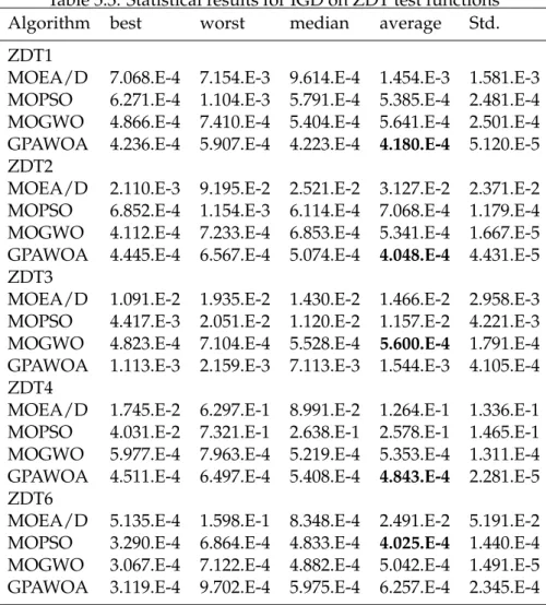
5.2 Best Pareto fronts produced by GPAWOA, MOEA/D, MOGWO and MOPSO of ZDT1 test function . . . 68
5.3 Best Pareto fronts produced by GPAWOA, MOEA/D, MOGWO and MOPSO of ZDT2 test function . . . 69
5.4 Best Pareto fronts produced by GPAWOA, MOEA/D, MOGWO and MOPSO of ZDT3 test function . . . 69
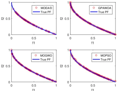
5.5 Best Pareto fronts produced by GPAWOA, MOEA/D, MOGWO and MOPSO of ZDT4 test function . . . 70
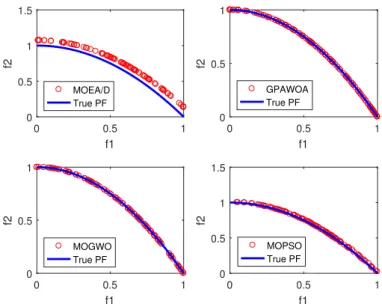
5.6 Best Pareto fronts produced by GPAWOA, MOEA/D, MOGWO and MOPSO of ZDT6 test function . . . 70
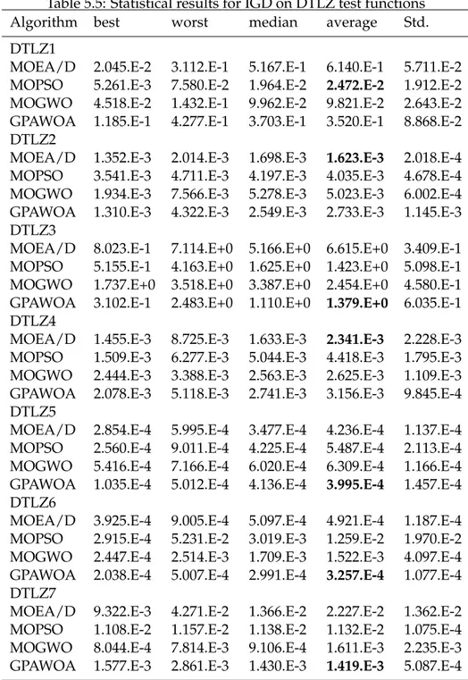
5.7 Best Pareto fronts produced by GPAWOA, MOEA/D, MOGWO and MOPSO of DTLZ1 test function . . . 73
5.8 Pareto front of DTLZ2: a comparison of the front found by
List of Figures vii
5.9 Best Pareto fronts produced by GPAWOA, MOEA/D, MOGWO and
MOPSO of DTLZ3 test function . . . 74
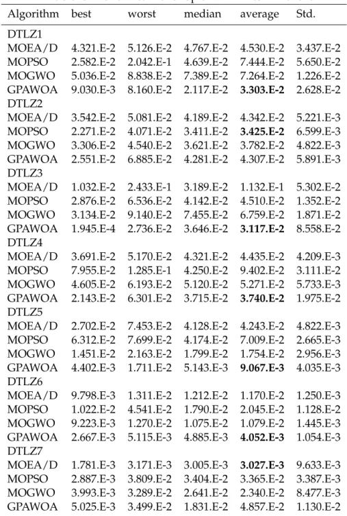
5.10 Pareto front of DTLZ4: a comparison of the front found by MOEA/D, MOGWO, MOPSO, GPAWOA and the true Pareto front . 75 5.11 Pareto front of DTLZ5: a comparison of the front found by MOEA/D, MOGWO, MOPSO, GPAWOA and the true Pareto front . 75 5.12 Pareto front of DTLZ6: a comparison of the front found by MOEA/D, MOGWO, MOPSO, GPAWOA and the true Pareto front . 76 5.13 Pareto front of DTLZ7: a comparison of the front found by MOEA/D, MOGWO, MOPSO, GPAWOA and the true Pareto front . 76 5.14 Four bar truss problem . . . 79
5.15 Gear train problem . . . 80
5.16 Disk brake design problem . . . 80
5.17 Welded beam design problem . . . 81
5.18 Comparison of nondominated solutions obtained by MOEA/D, GPAWOA, MOPSO and MOGWO for the 4-bar truss . . . 83
5.19 Comparison of nondominated solutions obtained by MOEA/D, GPAWOA, MOPSO and MOGWO for the Gear train . . . 84
5.20 Comparison of nondominated solutions obtained by MOEA/D, GPAWOA, MOPSO and MOGWO for the Disk brake . . . 84
5.21 Comparison of nondominated solutions obtained by MOEA/D, GPAWOA, MOPSO and MOGWO for the Welded beam. . . 85
List of Tables
5.1 Characteristics of multi-objective test functions . . . 65
5.2 Parameters of algorithms. . . 65
5.3 Statistical results for IGD on ZDT test functions. . . 66
5.4 Statistical results for Sp on ZDT test functions. . . 67
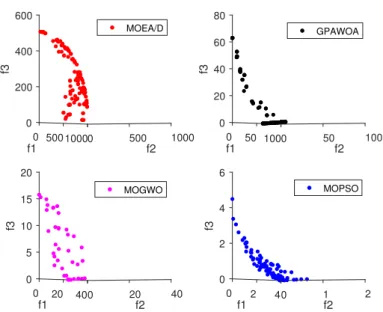
5.5 Statistical results for IGD on DTLZ test functions . . . 71
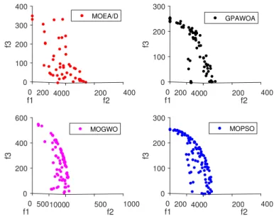
5.6 Statistical results for Sp on DTLZ test functions . . . 72
5.7 The p values of Wilcoxon test for IGD metric . . . 78
5.8 The p values of Wilcoxon test for spacing(Sp) metric . . . 78
5.9 Results of set coverage metric of the four engineering design problems 83 6.1 Summary of utilized datasets . . . 90
6.2 Parameter settings . . . 91
6.3 Experimental results of FW-GPAWOA, BDE, BPSO and BGWO . . . 91
6.4 The results of HV metric of FW-GPAWOA, MOGWO and MOPSO . 95 6.5 The p values of Wilcoxon test for HV metric . . . 96
6.6 The average running time consumed by the algorithms (unit: min-utes). . . 96
C
HAPTER1
Introduction
Contents
1.1 Overview . . . . 1
1.1.1 From machine learning towards optimization problem . . . . 1
1.1.2 Multiobjective feature selection for classification . . . 3
1.2 Motivations . . . . 5
1.3 Major contributions . . . . 6
1.4 Thesis organization . . . . 6
1.5 Academic publications . . . . 7
1.1
Overview
The present chapter introduces this thesis. It starts with a brief overview in which the relationship between machine learning and optimization problem is clarified, consequently, some multiobjective optimization methods for machine learning will be presented. Then, it outlines the motivations, the major contributions and the organization of the thesis.
1.1.1 From machine learning towards optimization problem
Historically, the term of machine learning has been known as the development of computers (machines in broader sense) able to learn and reasone automatically. That is to say, able to improve without the intervention of human. This ability for self-learning is done through experience and analytical observation. In [Nguyen 2008] denoted ”Broadly speaking, machine learning is the process of f inding and describing structural patterns in a supplied dataset”.
Machine learning algorithm is the tool that helps machines to evolve automati-cally and accomplish complex tasks that cannot done with classical algorithms. A machine learning algorithm can be defined as the process which takes as input a
2 Chapter 1. Introduction
dataset (also known as sample learning or examples) and provides as output the description of the knowledge that has been learnt. Generally speaking, machine learning algorithms can be classified into two main categories: unsupervised (often known as clustering) and supervised learning (often known as classifi-cation). The first category consists of finding patterns in the data above and beyond what would be considered pure unstructured noise [Ghahramani 2003]. In the second category, the aim is to create knowledge structures that predict and classfiy unknown information into predefined classes [Nguyen 2008]. Usually, the result of any classification algorithm can be viewed as a function (also called model) which approximate the mapping between the output and a new input dataset. So, the objective is to build a learning model that enable to a machine to predict the appropriate output of dataset without being explicitly programmed. However, the approximation quality can be affected by several factors. Indeed, the presence of irrelevant and redundant features results in poor accuracy of the model. Consequently, it is often desirable to identify the most informative features - a process known as feature selection (also known as dimensionality reduction).
Feature selection is considered as one of the major key in machine learning. The feature space usually contains a large number of features which can be divided into relevant/irrevelant features and redundant/non-redundant features. Irrelevant and redundant features are not useful as they affect the performance of a classification/learning algorithm [Russell 2003]. Therefore, feature selection technique is invoked to select the subset of relevant features in order to: decrease the dimensionality of the feature space, simplify the learning model, improve the classification performance and reduce the running time [Dash 1997]; [Liu 1998]. However, the high dimensionality of feature space imply high computational time. For n features, there are 2nsubsets possible. In addition, due to the absence of prior knowledge about the features and the complex interaction between them, the feature selection process is considered as an NP-hard problem.
Although there exist several feature subsets that can reduce the dimensionality of the search space, but the optimal subset is the one which contains smaller number of features and achieved better classification performance [Xue 2014b]. From broadly point of view, two main challenges are taken into account in order to select the optimal feature subset [Xue 2014a]. The first goal is to reduce as well as possible the size of feature space, and the second goal is to increase as well as possible the classification accuracy. Accordingly, feature selection is considered as a multiobjective optimization problem in which we attempt to minimize the number of features and maximize the classification performance. Further, these two criteria (number/performance) are often conflicting to each other and they
1.1. Overview 3
require simultaneous optimization.
Feature selection algorithms are usually grouped into two main categories: filter and wrapper approaches [Kohavi 1997]. Filter approaches use statistical measures to evaluate the quality of the selected feature subset, whereas wrapper approaches use a learning algorithm (or classifier) to evaluate the goodness of the selected features.
According to this brief state-of-the-art, we can say that the process of selecting an optimal feature subset is a crucial key to build hight-quality machine learning model. Additionally, we can say that the process of feature selection is performed through the resolution of a multi-objective optimization problem by using meth-ods propre for performing simultaneous optimization. In this thesis, we have chosen metaheuristic approaches based on the collective intelligence of a set of individuals to extract knowledge and overcome the complex difficulty to find the optimal solution.
1.1.2 Multiobjective feature selection for classification
This section attempts to provides a brief survey of multiobjective feature selection for classification.
Multiobjective optimization problem (MOP) involves optimizing several conflicting objective functions and possesses a set of solutions rather than single solution. The aim of any resolution method is on the one hand, to find the tradeoff non-dominated solutions called Pareto solutions (known as Pareto front), and on the other hand, to obtain well distributed Pareto solutions in order to maintain the diversity in the search space [Deb 2014]. In the literature, many multiobjective optimization algorithms such as non-dominated sorting genetic algorithm (NSGA) [Srinivas 1994], non-dominated sorting genetic algorithm 2 (NSGA2) [Deb 2002a], non-dominated sorting particle swarm optimizer (NSPSO) [Li 2003], Multi-Objective Artificial Bee Colony (MOABC) [Akbari 2012] have been proposed. The effectiveness of these algorithms for solving any multiobjective problem has encouraged researchers to apply them for tackling feature selection problems.
In [Hamdani 2007], a wrapper feature selection algorithm using NSGA2 is de-veloped. This algorithm attempts to minimize both the classification error and the number of features. K-Nearest Neighbours (KNN) algorithm was incorporated as classifier to evaluate the goodness of the selected feature subset. In [Xue 2012a], two binary multiobjective PSO frameworks were first developed. The first called
4 Chapter 1. Introduction
NSBPSO by using the NSPSO. The second called CMDBPSO by incorporating the ideas of crowding, mutation and dominance into PSO algorithm. Then, based on NSBPSO and CMDBPSO, four filter feature selection approaches are proposed which are: NSfsMI, NSfsE, CMDfsMI and CMDfsE. All these four approaches have the same goal which is: minimize the number of features and minimize the classification error rate. Since that they are filter-based approaches, mutual information and entropy are used as evaluation criteria. Compared against single-objective feature selection approaches, the results showed that the proposed multiobjective approaches perform better. Other multiobjective wrapper-based algorithms have been proposed by [Xue 2012b] called NSPSOFS and CMDPSOFS. Since that the two algorithms are wrapper approaches which need a classification algorithm to evaluate the performance of the selected subset, both NSPSOFS and CMDPSOFS utilize KNN algorithm (with K=5) as classifier. The results showed that CMDPSOFS algorithm can evolve a Pareto front which include a smaller number of features and achieve lower classification error rate. In [Hancer 2015], the MOABC algorithm is investigated to develop three filter-based feature selection approaches. Therefore, three filter evaluation criteria are used which are mutual information, fuzzy mutual information and new fuzzy mutual information proposed by the authors. The developed approaches are compared against three single-objective feature selection approaches and the results showed that the proposed methods perform better in terms of classification accuracy and especially in terms of the number of features. Recently, Grey Wolf Optimizer (GWO) [Mirjalili 2014] was investigated to propose new wrapper-based feature selection approach to improve the classification of cervix lesions [Sahoo 2017]. To achieve this, a non-dominated sorting based-GWO is developed to minimize the number of textural features and maximize the classification accuracy of cervix lesions. By the fact that the proposed algorithm (called NSGWO) is wrapper approach, Support Vector Machine (SVM) is employed as learning algorithm to evaluate the selected feature subset. Based on NSGA algorithm, [Waqas 2009] propose a new wrapper approach for feature selection. ID3 decision tree al-gorithm was employed as classifier to evaluate the fitness of each individual. In [Xue 2014a], two filter-based multiobjective feature selection approaches are proposed called MORSN and MORSE to obtain the set of non-dominated feature subsets. To achieve this goal, rough set (RS) [Pawlak 1995] is used to construct two measures: the first measure is to evaluate the classification performance and the second is to evaluate the number of features.
1.2. Motivations 5
1.2
Motivations
After the presentation of the concept of feature selection, its high importance and its influencing in machine learning, and after showing the relationship between a feature selection problem and a multiobjective optimization problem, including the presentation of some feature selection algorithms. We summarize the main motivations of our work in the following points:
• The tremendous usefulness of machine learning techniques in todays society and for everyday life. Medical diagnostics, marketing and airport security are some examples in which machine learning has had remarkable success.
• Addressing feature selection problem as it is one of the most important task in machine learning. Feature selection is a complex problem in which it is too expensive to discover entire the feature space. Therefore, the search for an optimal feature subset is NP-hard problem for which we don’t know any exact approach that can select only the needed features in acceptable running time.
• Addressing the feature interaction problem. Indeed, the difficulty of feature selection problem is not only due by the fact that the search space is very large, but also by the fact that the features are highly interacting between them. A given feature may be irrelevant, but when it is combining with other feature, it can becomes extremely relevant and very informative.
• Addressing feature selection as a multiobjective optimization problem. Although there exist some multiobjective appoaches for solving feature selection problem, but in the literature, there are rare approaches that handling feature selection as a multiobjective problem compared to those that handling it as single-objective problem.
• Taking advantage of metaheuristics based on the evolution of a population of solutions which offer a high ability to explore a large part of the srach space in reasonable computational time and overcome the problem of local optimal feature subset.
6 Chapter 1. Introduction
1.3
Major contributions
To solve feature selection problems using metaheuristics methods, our contribu-tion is made in two phases:
• The first phase consists of developing a resolution approach as a new alter-native to solve multiobjective optimization problems in a general manner.
• The second phase is to investigate the proposed approach for developing a new feature selection algorithm.
In the first contribution, we have proposed a new multiobjective optimization algorithm called GPAWOA (for Guided Population Archive Whale Optimization Algorithm). The proposed algorithm extend a recent single-objective algorithm called Whale Optimization Algorithm (WOA) in ordre to be able to deal with multiobjective optimization problem. The GPAWOA incorporates the Pareto optimality concept into the standard WOA and uses an additional population (archive) to guid the search towards the true Pareto front. In addition, the mechanism of crowding distance is adopted in two steps of the algorithm in order to obtain distributed solutions. The GPAWOA was evaluated using 12 well-known benchmark functions (5 bi-objective test functions and 7 three-objective test functions). Moreover, it was applied to four multiobjective engineering design problems. The exprimental results showed that the proposed GPAWOA is highly competitive compared against existing multiobjective optimization algorithms, being able to provides an excellent approximation of Pareto front in terms of convergence and diversity.
In the second contribution, we have applied the proposed GPAWOA for solving feature selection problem. This contribution consists of hybriding filter and wrapper models into a single system at the hope to benefits from the merits of each model. The proposed algorithm demonstrated its ability to be a good alternative for handling effectively the feature selection problems.
1.4
Thesis organization
The remainder of this thesis is organised as follows:
Chapter 2 gives a brief review of machine learning and presents some well-known classification algorithms. Also, it provides a short review of feature
1.5. Academic publications 7
selection problem, including the key steps of any feature selection approach and the main types of feature selection algorithms.
Chapter 3 provides a generality of optimization problems. It starts with the definition of the complexity theory and single-objective optimization problems. Then, it presents some exisitng resolution methods, in particular, the metaheuris-tics that use a population of solutions.
Chapter 4 presents the essential background and basic concepts of multiobjec-tive optimization problems. It provides the essential notions and in particular the dominance Pareto concept. Also, it gives the main challenges of multiobjective problems. In addition, it reviews typical and popular resolution approaches.
Chapter 5 presents the proposed GPAWOA algorithm for solving multiobjec-tive optimization problems. First, it gives a detailed description of GPAWOA algorithm, including the mechanisms used and the archiving strategy adopted in the algorithm and its pseudocode. Finally, it provides a summary of an extensive experimental evaluation.
Chapter 6 devoted to the description of the proposed FW-GPAWOA algorithm for feature selection. It provides how FW-GPAWOA treat discrete problems and how combining filter and wrapper approaches. Finally, it provides a summary of the comparative study.
Chapter 7 summaries the work and attractions overall conclusions of the thesis. Main research ideas and the contributions of the thesis are established as well. It also suggests some possible future research directions.
1.5
Academic publications
• Got Adel, Abdelouahab Moussaoui, and Djaafar Zouache. "A guided population archive whale optimization algorithm for solving multiobjective optimization problems." Expert Systems with Applications 141 (2020):
112972. https://doi.org/10.1016/j.eswa.2019.112972, impact
factor: 5.452.
• Got Adel, Abdelouahab Moussaoui, and Djaafar Zouache. ”Hybrid filter-wrapper feature selection using Whale Optimization Algorithm: A Multi-Objective approach”. Expert Systems with Applications (Under review), impact factor: 5.452.
C
HAPTER2
Machine learning and feature
selection
Contents
2.1 Introduction . . . . 8
2.2 Supervised learning . . . . 9
2.2.1 K-nearest neighbor algorithm (KNN) . . . 10
2.2.2 Support Vector Machine (SVM) . . . 11
2.3 Unsupervised learning . . . . 13
2.3.1 k-means algorithm . . . 13
2.3.2 Hierarchical clustering algorithm (HCA) . . . 14
2.4 Dimensionality reduction based on feature selection. . . . 15
2.5 Feature selection problem . . . . 16
2.6 General procedure of feature selection algorithm . . . . 16
2.6.1 Generation procedure . . . 17 2.6.2 Evaluation procedure . . . 18 2.6.3 Stopping criteria . . . 20 2.6.4 Validation . . . 20 2.7 Chapter summary. . . . 20
2.1
Introduction
Machine learning is a subfield of Artificial Intelligence (AI) which consists in building from a set of sample data, a learning model that allows to a machine to self-learning, that is to say, to analyze and reason in an autonomous manner with complex data. This ability to learn automatically from analytical observation of the sample data results in obtaining an intelligent artificial system able for learning and adapting with new datasets without being explicitly programmed.
2.2. Supervised learning 9
Therefore, machine learning refers to the development of methods that enable to a machine to evolve automatically and accomplish tasks which are complex for classical algorithms.
In general, the process of a learning algorithm is divided into two phases [Aggarwal 2014]. The first phase (learning phase) consists to generate a prediction model ready to the implementation for the future situations. The second phase (deployment phase) consists of applying the generated model on the datasets to accomplish the desired tasks (usually is decision-making). Its clear that the quality of the final decision is strongly depends on the performance and the accuracy of the generated learning model. In addition, the input space (dataset) of a learning algorithm is often divided into a training space and testing space [Muñoz 2018]. The training space constitutes the set of examples used to provide the learning model, while the testing space is used to check the performance of the generated model.
Although there exist several types of machine learning, however, supervised and unsupervised learning that we will present in the following sections, are the most known types of machine learning and they are the most studied in the literature.
2.2
Supervised learning
Supervised learning consists in generating a typical prediction model connecting the predictor variables X and a target variable Y predetermined beforehand. A supervised learning algorithm takes as input a sample data (training set), where each data examples is assigned to a categorized variable called the target class (label). The goal is to build a learning model able to predict with high accuracy the target classes of new data examples (unseen datasets) that are not belong to the learning sample [Dougherty 1995].
Formally, given a training set D containing m example, where each example Ei is represented by the input xiand its associated output target yi:
D = {Ei/Ei = (xi, yi), xi ∈ X and yi ∈ Y, i = 1, 2, 3, ..., m} (2.1) The objective is to build a learning model called hypothesis function h(x) = y with x /∈ X, able to predict for any given input datum x, the value of the output target y. Depending on the nature of the output target Y , there are two types of supervised learning problems:
10 Chapter 2. Machine learning and feature selection
• Supervised classification if the target variable Y takes discrete values (binary, boolean, ect.). For a classification problem, Y corresponds to a finite number of classes used to find the model that classifiy the unseen datasets.
• Regression problem if the output target Y is continuous value. There are several regression forms, the simplest is the linear regression. It tries to fit data with the best hyperplane which goes through the points. Therefore, the learning model will be a simple straight line.
2.2.1 K-nearest neighbor algorithm (KNN)
The k-nearest neighbor algorithm (KNN) is considered to be one of the simplest supervised classification algorithms [Indyk 1998]. Its principle is to assign the input data to the most represented class among its k-nearest neighbors in terms of distance as shown in figure2.1.
Figure 2.1: K-Nearest Neighbor classification algorithm
Given a new unlabeled vector x, the KNN algorithm consists in finding the set E containing k-closest classes to x, and by majority vote, it determines the most frequent class in E and assigns it the new vector x.
2.2. Supervised learning 11
choosing smaller k can be less immunized against the noise in the learning sample, a large value of k makes it difficult to define the limits between classes.
There are many variants of this algorithm depending on the distance calcu-lation function used [Chomboon 2015], usually the most used is the Euclidean Distance. The major advantage of the k-nearest neighbor method is its simplicity and ease of implementation. On the other hand, the high cost when searching for neighbors is its main drawback, especially in large databases. In addition, the choice of k-value might be not obvious.
2.2.2 Support Vector Machine (SVM)
Support Vector Machine method is based on the theoretical work of Vanpik and Cortes [Cortes 1995]; [Boser 1992]. SVMs are usually used for classification models and applied to linearly and non-linearly separable problems. The objective is to find the optimal separating hyperplane among an infinity of hyperplanes, which linearly separates the learning sample by maximizing the margin (in terms of distance) between the separating hyperplane and the closest points to the limit of separation (see figure2.2). These points are called support vectors.
Figure 2.2: Optimal hyperplane for Support Vector Machine with two classes SVMs are based on two concepts which are : the maximum margin and the kernel function. In the linearly separable case, the separating hyperplane is a simple straight line defined by the function h:
12 Chapter 2. Machine learning and feature selection h(x) = n X i=1 wi.xi+ b (2.2)
where, w is the normal vector of the hyperplane and b is the displacement from the origin.
As we have seen previously, the optimal hyperplane is the one which max-imizes the minimum distance between the separation limit and the support vectors. This distance is given as follows:
d(xi, h) =
yi.h(xi)
kwk (2.3)
with, yiis the corresponding class of any point xi.
Maximizing the distance d amounts to minimize the quantity kwk, which leads, after certain mathematical operations, to the following optimization problem:
minkwk22 yi.h(xi) ≥ 1, i = 1, 2, 3, ..., n (2.4) This problem can be solved using the lagrange multipliers method. Therefore, the hyperplane function for a new datum x is written as follows:
h(x) = n X
k=1
ak.yk.(x.xk) + b (2.5)
where akare the lagrange multipliers.
In the non-linearly separable case where there is no hyperplane able to sepa-rates the classes, SVM uses the so-called kernel f unction to transform the initial space into a higher dimension space φ in which there is a possibility to perform a linear separation. Accordingly, the function of the separating hyperplane is defined in the new space φ and it is given by:
h(x) = n X
k=1
ak.yk.K(x, xk) + b (2.6)
K(x, xk) is the kernel function. There are many kernel functions such as polynomial, gaussian and RBF kernel functions [Schölkopf 2002]. The SVMs have shown their ability to provide excellent performance in classification problems, and they have been employed in several areas such as the pattern recognition [Byun 2002] and medical diagnostics [Pimple 2016]; [Sweilam 2010].
2.3. Unsupervised learning 13
2.3
Unsupervised learning
Unlike the supervised learning where the database is labeled, unsupervised learning is used when the learning sample contains only raw data (unlabeled ex-amples). That is to say, the target classes including their numbers are not defined a priori. Consequently, this type of problem is often more difficult compared to supervised problem.
An unsupervised algorithm consists in finding patterns or clusters that group the dataset based on certain similarity between the data. Therefore, the goal is to discover the target classes that maximize the intra-class similarity and minimize the inter-class similarity [Jain 2000]. Various tasks are associated to this type of learning, in particular, the clustering which involves grouping the dataset into several classes called clusters, where each cluster is a collection of similar objects. Usually, this similarity criterion is expressed in terms of distance function.
2.3.1 k-means algorithm
The k-means method proposed in [MacQueen 1967] is one of the most popular clustering algorithms in the current usage as it is relatively fast and simple to understand and easy to deploy in practice. As illustrated in figure 2.3, k-means algorithm consists of partitioning the dataset into K clusters, such that objects within the same cluster are similar as well as possible, while the objects from different clusters are dissimilar as well as possible. In k-means algorithm, each cluster is represented by its center (centroids) that corresponds to the mean of points assigned to the cluster. The k-means algorithm is given in the following steps [Selim 1984] :
1. Determine the number K of clusters Ci.
2. Initialize randomly from the data points, K centroids (denoted wi).
3. Assign each data point to the closest cluster (centroid).
14 Chapter 2. Machine learning and feature selection V = k X i=1 X wi∈Ci D(xi, wi)2 (2.7)
with, xi is the point belongs to the cluster having the centroid wi and D(xi, wi)is the Euclidean distance between wiand xi.
5. If the partitioning does not converge, return to 3.
Figure 2.3: Example of clustering using K-means algorithm
The good accuracy and efficiency of the K-means algorithm motivate re-searchers to propose several variants such as K-medians [Juan 2000], K-medoids [Park 2009] which applied different techniques to calculate the centroids of clusters.
2.3.2 Hierarchical clustering algorithm (HCA)
Hierarchical clustering algorithm (also known as hierarchical cluster analysis) is a classical clustering algorithm which consists for grouping two individuals or two groups (clusters) of individuals that are closest together in terms of distance until all objects are grouped into a single cluster [Ward Jr 1963]. The result of this type of algorithm is usually represented as a hierarchical tree (or dendrogram). In order to obtain the desired classes, a division at a certain level of the dendrogram must be performed (see figure2.4).
2.4. Dimensionality reduction based on feature selection 15
Figure 2.4: Dendrogram for the Hierarchical Cluster Analysis (HCA) Let A = {a1, a2, ..., an} be the set of individuals to be grouped, HCA algorithm takes place in the following way:
1. Initialize the clusters Ciwhere each cluster contains a single individual of A.
2. Combine the nearest clusters Ciand Cjto form a new cluster Ck.
3. Calculate the distance between Ckand the clusters Cywith y 6= i, j.
4. Repeat 2 and 3 until the aggregation of all individuals of A into a single cluster.
2.4
Dimensionality reduction based on feature selection
In practice, the performance of any learning algorithm does not depend only to its design and its manner to deal with the set of data. Indeed, several factors can affect the quality of the algorithm, including the representation and quality of the dataset. High dimensionality of data, the existence of irrelevant and redundant data (features) are some factors which could decrease the algorithm performance [Dash 1997]. Consequently, it is often necessary to reduce the dimensionality of the sample learning (dataset) in order to remove the irrelevant and redundant
16 Chapter 2. Machine learning and feature selection
features. Generally, the dimensionality reduction strategies are grouped into two categories :
• Reduction by feature selection, which consists to select the most relevant features from the dataset.
• Reduction by feature extraction, which attempts to transform the initial space to lower dimensional space. Principal Component Analysis (PCA) is one of the typical methods for dimensionality reduction based on feature extraction [Jolliffe 2016].
In our thesis, we’re interested on the reduction through the use of the feature selection technique. For this reason, a brief overview on the feature selection problem will be presented in the following sections.
2.5
Feature selection problem
Feature Selection is one of the core concepts in machine learning which try to select the most informative (relevant) variables or attributes from highly dimensional data. It is a technique widely used to reduce the size of the datasets while building the subset containing the features deemed relevant. The impact of the feature selection is not limited only to the dimensionality reduction, but extends to the construction of an efficient and simplest learning model. Hence, improving the performance of the system and optimizing the running time [Langley 1994]. The feature selection problem is the process of finding, from the original features, the optimal subset that is sufficient for solving successfully a classification problem. The optimal feature subset is the minimum subset that can provide the better classification accuracy, which makes feature selection a multiobjective problem [Xue 2012b]; [Oliveira 2002].
2.6
General procedure of feature selection algorithm
According to [Dash 1997], a typical feature selection algorithm includes the four key steps illustrated in figure2.5. The search process starts by generating the
can-2.6. General procedure of feature selection algorithm 17
didate feature subsets which will be evaluated by using a certain evaluation cri-terion. These two steps are repeated until a given stopping criterion is satisfied. Finally, a result validation step is applied to validate the selected feature subset.
Figure 2.5: Four key steps of feature selection algorithm [Dash 1997]
2.6.1 Generation procedure
The generation procedure (also called search procedure) consists of creating a subset of candidate features from the initial set of features. However, for a given set containing N features, there are 2N possible subsets, which makes an exhaustive search very expensive even impossible for a large number of features. Therefore, three search strategies have been proposed [Liu 2005]:
• Complete search
This strategy can provides the guarantee of finding the best feature subset according to the employed evaluation criterion. An exhaustive search is absolutely complete while a non-exhaustive search can be complete. This is possible by using different heuristic functions to reduce the search space without compromising the chances of finding the optimal subset by applying backtracking process (Branch and bound for example) allowing to go back if the selection is going in the wrong generation direction.
• Sequential search
Also called heuristic search, the principle of sequential search is to add or delete, iteratively, one or more features. It begins either with an empty set
18 Chapter 2. Machine learning and feature selection
and then the features are added one at a time until a stopping criterion is reached (sequential forward selection SFS), either by the original set and then eliminates features one at a time (sequential backward selection SBS). A third search strategy (sequential stepwise selection) consists for combining the previous strategies while removing or adding the features from the selected subset.
• Random search
As its name indicates, the random search (also called stochastic search) consists of randomly generating a finite number of candidate features. The methods based on such strategy (such as genetic algorithm) are able for escaping from local optima subset and reducing the running time.
2.6.2 Evaluation procedure
In this step, an evaluation criterion is defined in order to measure the quality of each features subset generated in the previous step. Obviously, the choice of the evaluation function is crucial to obtain an optimal subset. The generated subset using a given evaluation criteria may be not the same using another evaluation criteria [Xue 2014b]. Additionally, according to the used evaluation criterion, the feature selection algorithms can be classified into two main categories : Filters and Wrappers.
• Filter approach
In filter methods, the evaluation is realized without involving any mining algorithm, which means that the evaluation is independent to the used classifier. Several measures criterion are proposed to evaluate the goodness of the candidate features. Consistency, mutual information, correlation criteria and rough set theory are usually the most employed filter functions in the literature [Dash 2003]; [Chandrashekar 2014].
Filter algorithms are known as fast to compute and easy to understand. However, the ignorance of features dependency and the absence of interac-tion with the classifier are the main disadvantages of filtering methods.
2.6. General procedure of feature selection algorithm 19
Figure 2.6: Overall schematic of filter method
• Wrapper approach
In contrast of the filter methods which try to find the optimal feature subset independently of the classification algorithm, the wrapper methods integrate the classifier to search and evaluate the candidate feature subset, which re-sults in increasing the chance to obtain a better subset.
In general, the use of wrapper methods make it possible to obtain a high accuracy comparing to filter methods thanks to the well interaction of the selected features with the classifier. However, the big shortcoming of these methods is they require high computational costs even when using simple classification algorithm.
20 Chapter 2. Machine learning and feature selection 2.6.3 Stopping criteria
Generally, the number of features to be selected is unknown a priori, which makes the definition of a good stopping criterion a crucial step while ensuring the selec-tion of the needed features. In fact, a poor choice of the stopping criterion can force the selection process to stop while the optimal subset is still far away. In practice, the choice of stopping criterion depends on the search strategy and the evalua-tion funcevalua-tion. Among the most used stopping criteria in the literature, we can cite :
– Predefined number of features to be selected (knowing that this task is not often achievable as mentioned previously).
– Predefined number of iterations is reached (this type of criterion can reduce the computational costs but the result is not necessarily optimal).
– Addition or deletion of any feature does not result in a better subset. – An optimal subset is obtained (for example, given error rate is allowable).
2.6.4 Validation
The result validation is considered as the fourth and the final step in the feature selection process. It depends on the nature of handled dataset, artificial or real. A straightforward way for validation is to directly measure the quality of the obtained features subset. In this case, prior knowledge about the relevant features is necessary. The database benchmarks are typically used to directly validate the obtained results.
In real-world applications, generally there is no prior knowledge about the relevant features. In this case, the validation process utilize some indirect methods by observing the change of the performance indicator (such as classification error rate) with the change of features subset [Liu 2005]. Cross-validation technique might be also used to assess the performance of the selected feature subset.
2.7
Chapter summary
In this chapter, we have presented the basic concepts of machine learning and its main types; supervised and unsupervised learning, as well as their operating principles and some algorithms for each type.
2.7. Chapter summary 21
which is the dimensionality reduction, in particular, the reduction based on the feature selection. Consequently, a brief overview for feature selection is given in which we have presented the main steps to be taken into account when designing any feature selection algorithm. In addition, feature selection approaches, namely: filter and wrapper algorithms were presented, including the advantages and disadvantages of each model.
C
HAPTER3
Generalities on the optimization
problems
Contents 3.1 Introduction . . . . 22 3.2 Complexity theory . . . . 23 3.3 Optimization problems . . . . 24 3.3.1 Mathematical formulation . . . 253.3.2 Resolution of optimization problems. . . 25
3.4 Optimization exact methods . . . . 26
3.4.1 Linear programming . . . 26
3.4.2 Branch and Bound (B and B) . . . 27
3.5 Single solution based metaheuristics . . . . 28
3.5.1 Tabu Search . . . 28
3.5.2 Simulated Annealing . . . 29
3.6 Population based metaheuristics. . . . 30
3.6.1 Genetic Algorithm (GA) . . . 30
3.6.2 Particle swarm optimization (PSO) . . . 32
3.6.3 Ant colony algorithm (ACO) . . . 33
3.6.4 Whale Optimization Algorithm (WOA) . . . 35
3.7 Chapter summary. . . . 37
3.1
Introduction
Currently, the optimization has become an important multidisciplinary field that can be used in image processing, engineering design, machine learning, bioin-formatics, economics, etc. The researchers, decision-makers and engineers are often faced against high-dimensional problems that might requires an exhaustive
3.2. Complexity theory 23
search, which is not always feasible in a reasonable time.
An optimization problem can be defined as the act of finding the best result among the set of all feasible solutions. However, most of these problems are NP-hard where there is no exact resolution method that can find the best solution in reasonable computation time. Without claiming to be an exhaustive presentation, we will present in this chapter the main optimization concepts. Hence, some resolution methods will be presented, in particular, the so-called ”metaheuristics”.
3.2
Complexity theory
For a given problem, there are several algorithms that can be used for solving it, and the user is faced with the following question: among this multiplicity of al-gorithms, which algorithm is performing better ?. The straightforward way to answer this question is to compare the running time of each algorithm. However, this comparison is unfair because it is affected by several factors such as the char-acteristics of the machine in which the algorithms are implemented. Therefore, other approach independent of any software and hardware resources is necessary to perform rigorous and an equitable comparison.
The complexity of an algorithm can be defined as the estimation of necessary number of elementary operations performed by this algorithm to solve a given problem. The complexity theory consists [Papadimitriou 2003]; [Arora 2009] of formally studying the difficulty of a decision problem whose the answer is of bi-nary type (yes/no, true/false, 0/1, ect). Furthermore, some studies [Cook 1971]; [Karp 1972] have shown that there is a fundamental classification of optimization problems based on the complexity of the algorithms used for solving them.
Définition 3.1 (P class) We distinguish by P class the problems that can be solved
efficiently by an algorithm of polynomial complexity, that is to say in O(Np)where N is the size of the problem and p is a constant.
Définition 3.2 (NP class) The NP class involves the problems that can be solved by a
non-deterministic algorithm in polynomial time. Moreover, the correctness of a claimed solution can be checked in polynomial time. From this definition, it is clear that the inclusion P ⊂ NP is valid, but the reverse was never been affirmed.
24 Chapter 3. Generalities on the optimization problems
Définition 3.3 (NP-complete class) This class contains NP problems that are
consid-ered more difficult than any other NP problem. A problem Q known to be NP-complete if it is in NP and if any NP problem can be reduced to Q in polynomial time. Among the well-known NP-complete problems we can cite: the boolean satisfiability (SAT) and knapsack problem.
3.3
Optimization problems
Each optimization problem is characterized by its search space, an objective function and a set of constraints:
• The search space is the set of the feasible solutions and it is defined by a finite set of decision variables, each of them with a finite domain.
• The objective function represents the goal to be reached (minimizing the cost, the error rate, or maximizing the profit, the measure, etc.) according to the problem context.
• The constraints are the set of conditions that should be respected during the optimization process. They are often of inequality or equality equations and they allow to boundary the search space.
An optimization problem is defined as the act of searching within the search space, the solution that minimizes (or maximizes) the objective function while sat-isfying the constraints. This solution is called optimal solution or the global opti-mum. However, for a given optimization problem, a candidate solution might be optimal for a part of search space but not for all the search space: we talk about local optima and global optima. These two notions are illustrated in figure3.1.
3.3. Optimization problems 25
Figure 3.1: Illustration of local optimum and global optimum
3.3.1 Mathematical formulation
Mathematically, an optimization problem is formulated as follows: min f (x) gi(x) ≤ 0, i = 1, 2, 3, ..., m hj(x) = 0, j = 1, 2, 3, ..., k xL≤ x ≤ xU (3.1)
where x ∈ S is the vector of decision variables and S is the search space, f (x) is the objective function to optimize, gi and hj are, respectively, the inequality and equality constraints. xLand xU are, respectively, lower and upper bounds of decision variables. The aim is to find the point x∗that satisfy the constraints gi, hj and ∀x ∈ S , f (x∗) ≤ f (x)[Schoen 1991].
3.3.2 Resolution of optimization problems
The main objective when solving optimization problems is finding the global optima rather than the local optima. In order to achieve this goal, an exploitation strategy of the search space must be defined [Chen 2009]. Additionally, due to the existence of several local optima, an exploration strategy is necessary to overcome the local optimality problem [Xu 2014]. The exploration attempts to visit a large
26 Chapter 3. Generalities on the optimization problems
part of the search space, while the exploitation express the ability of the resolution method to focus in the regions that probably containing an optimal solution. According to this description, we can say that the performance of such resolu-tion method depends on the manner to deal with the exploraresolu-tion/exploitaresolu-tion dilemma.
In the literature, there exist several solution methods which are usually catego-rized into exact and approximate (metaheuristics) approaches [Talbi 2009]. In the following, some existing methods will be presented.
3.4
Optimization exact methods
The exact approaches include all algorithms which are guaranteed to find an optimal solution and to prove its optimality for every instance of the combina-torial optimization problem [Puchinger 2005]. Generally, they take the form of exhaustive search. These methods have an exponential computational complexity, indeed, the time to solve the problem grow exponentially with its size.
3.4.1 Linear programming
Linear programming (also called linear optimization) is a decision mathematical support tool which is dedicated for solving optimization problems whose the ob-jective function and the constraints are in the form of a system of linear equations.
The general form of a linear program (LP) is given as: min f (x) =Pn i=1cixi Ax ≥ b xi ≥ 0, x ∈ Rn, A ∈ Rm∗n, x ∈ Rm (3.2)
with, ci are the coefficients of the objective function f (x), A and b are the matrix and vector, respectively, of constraints. x is the vector of decision variables. The solution of a linear program is a values assignment to the decision variables of the problem. The solution is feasible if it satisfy all the constraints. One of the well-known optimization algorithms in linear programming is the simplex algorithm [Bartels 1969].
3.4. Optimization exact methods 27 3.4.2 Branch and Bound (B and B)
Branch and Bound [Land 1960]; [Lawler 1966] is a technique usually used for solving combinatorial optimization problems. It consists of an enumeration systematic non-exhaustive of the solutions space while eliminating the subsets of solutions that does not lead to the desired solution. Its operating principle is inspired by the classic computer science paradigm ”Divide to conquer” and it is based on two concepts:
• Branching which is the process of spawning subproblems from the initial problem while building a ”decision tree” in which the nodes represent the sub-problems, each one is associated to a reduced solutions space.
• Bounding which attempts to guide the search tree by using the so-called ”lower” and ”upper” bounds. It consists to maintain the current subset as a potential search space, or pruning it if its associated bound is worse than the best known solution. The classical bounding strategies are; either browsing the decision tree in depth first (Deep-First Search), or in width first (Breadth-First Search), or handle the best subset not yet treated (Best-First Search).
Branch and Bound algorithm can obtains an optimal solution and enumerates the search space in acceptable complexity if the problem is of limited size. Due to its efficiency and simplicity, several variants have been proposed such as Branch and Cut [Padberg 1991] and Branch and Price [Barnhart 1998].
As mentioned above, the computational cost of exact approaches increase exponentially with the problem size. Thus, due to the ”combinatorial explosion” nature of the real-world problems, such approach is not efficient and even not applicable. In this case, the so-called ”metaheuristics” represent an interesting alternative which aimed at providing high-quality solution (instead of guaran-teeing a global optimum solution) in acceptable computing time [Gogna 2013]. Based on a stochastic search, the metaheuristics progress iteratively by alternating effectively between exploration and exploitation techniques in order to converge as well as possible towards the optimal solution. Many criteria may be used to categorized the metaheuristic, the classification of metaheuristics, which differentiates between Single solution-based and Population-based, is often taken to be a fundamental distinction in the literature [BoussaïD 2013].
28 Chapter 3. Generalities on the optimization problems
3.5
Single solution based metaheuristics
Single solution methods manipulate a single point of the search space throughout the progression of the algorithm. Also called trajectory methods, they start with a random initial solution and try to, iteratively, evolve and improve the current configuration in it local neighborhood while constructing a trajectory path within the search space. Tabu Search and Simulated Annealing are considered as the most popular single-based algorithms in the literature.
3.5.1 Tabu Search
Tabu search proposed by Glover in 1986 [Glover 1986] is a local search method that inspired by the human memory. In fact, Tabu Search (TS) utilizes an adaptive memory called tabu list in which the promising regions already visited are listed. This mechanism allows to prevent the search process to perform backwards moves to the solutions previously explored. The principle of Tabu search is the use of the neighborhood notion that consists in replacing the current solution by the best so-lution among all of its neighbors. However, this strategy may lead to a premature convergence. Therefore, Tabu search permits moves that deteriorate the objective function in ordre to overcome local optima.
Algorithm 3.1:Tabu Search algorithm
1 Initialize the tabu list T = ∅ 2 Choose an initial solution s
3 V (s): neighborhood of the current solution s
4 Sbest= s
5 while t < itermaxdo
6 Choose the best solution s0from V (s) 7 if f(s0) < f(Sbest) then
8 Sbest=s0
9 end
10 Update the tabu list T 11 s = s0
12 t=t+1
3.5. Single solution based metaheuristics 29 3.5.2 Simulated Annealing
Simulated Annealing (SA) is one of the simplest and effective method, it is based on the physical annealing process used by metallurgists [Kirkpatrick 1983]; [Cern `y 1985ˇ ]. Annealing aims to obtain homogeneous and well structured mate-rials by alternating slow cooling and heating cycles until reaching the thermody-namic equilibrium. A metal in the liquid state (at high-temperature) is a metal whose the atoms that compose it are unstable. The cooling act (lowering of tem-perature) enable to stabilize these atoms while minimizing their energies of dis-placement. However, the sharp cooling may unbalance the atoms. Hence, the lowering of temperature must be done in a regular and careful manner. This phys-ical phenomenon has been perfectly applied in Simulated Annealing algorithm to solve optimization problems where: the temperature becomes a control parameter and the energy becomes the objective function to be optimized [BoussaïD 2013].
Algorithm 3.2:Simulated Annealing algorithm
1 s ←initial solution
2 N (s): neighborhood of the current solution s 3 Sbest = s
4 T ← maxT emperature
5 while t > minT emperature do
6 iter ←0
7 while iter < M axIter do
8 Select a random solution s0from N (s) 9 ∆= f (s0) − f (s) 10 if ∆ < 0 then 11 s = s0 12 if f(s0) < f(Sbest) then 13 Sbest= s0 14 end 15 else 16 if rand(0, 1) < e −∆ T then 17 s= s0 18 end 19 end 20 iter = iter + 1 21 end 22 T ← T × (1 − α) 23 end
30 Chapter 3. Generalities on the optimization problems
At the start of the algorithm, the T parameter is initialized to a high value and the search begins with a random initial solution. At each iteration, another solution s0 is chosen from the neighborhood of the current solution s. If this solution improves the objective function, it will be accepted. Otherwise, it will be accepted but with a certain probability P which depends on T parameter. Indeed, P is higher whenever T is higher. Initially, T parameter is high enough in order to favored the exploration of the search space, thereby escaping from local optima. During the iterations, T parameter decreases and consequently, the probability P of accepting a degradation within the solution quality decreases. This mechanism improve the ability of the algorithm to focus on promesing regions while accepting only the configurations that enhance the objective function in order to converge to the optimal solution.
Due to its high ability to provides an excellent approximation of the global optima, Simulated Annealing algorithm has been successfully applied in several academic optimization problems [Elmohamed 1997]; [Malek 1989]; [Drexl 1988] and it has a broad range of real applications [Suman 2006].
3.6
Population based metaheuristics
Unlike single solution-based methods, population-based metaheuristics ma-nipulate a set of solutions called population and they are usually inspired by natural phenomena. These methods represent a powerful tool for solving different types of optimization problems thanks to their ability for perform-ing global search. Additionally, usperform-ing a population of solutions increase their ability to explore very large part of the search space in reasonable running time. In the following paragraphs, some population-based algorithms will be presented.
3.6.1 Genetic Algorithm (GA)
Genetic Algorithms (GAs) are considered as the well-known population-based metaheuristics belonging to the larger class of evolutionary algorithms (EAs). The origins of GAs dates back to the early 1970s in Holland’s work [Holland 1975] by inspiring the process of natural evolution of living things and genetics. Genetic algorithms simulate the Darwins theory of evolution ”survival of the fittest”: fitter organisms have a better chance of surviving and to produce offsprings to the next generation.
3.6. Population based metaheuristics 31
Without having delved too much into the genetic aspect, the best individuals (parents) of the current population are selected to produce offsprings by applying two genetic operators known as crossover and mutation. An individual (chromo-somes) is composed of a sequence of genes. The crossover allows to create new childrens by exchanging the genes of two parents, while the mutation is a random pertubation on the genes of the borne children. Finally, the fittest children’s re-place the weakest parents to generate new population, hopefully, better than the original parental population.
Despite the field of genetic algorithms was established by John Holland. How-ever, their mathematical formulations for solving optimization problems have been introduced by David Goldberg [Goldberg 1989].
Algorithm3.3provides the operating principle of GA. The population of indi-viduals (solutions) are maintained within the search space. For each individual is applied a fitness score, that is, the evaluation of the objective function. At each iteration, the best solutions are chosen by using a given selection strategy such as roulette wheel selection, rank selection and tournament selection (for more de-tails on selection schemes, you can see [Goldberg 1991]). Once the solutions are selected, crossover and mutation operators are applied with a certain probability in order to create an intermediate population. Mutation operators are mostly used to increase the exploration ability, whereas crossover operators are widely used to lead the population towards promesing points in the search space (i.e, increase the exploiatation ability of the algorithm). Finally, the fittest solutions in the in-termediate population are selected to replace the weakest solutions in the current population in order to reproduce a new population better than the old population.
Algorithm 3.3:Pseudocode of a Genetic Algorithm
1 Generate an initial random population P of individuals 2 gen = 0
3 while gen < GenM ax do
4 Evaluate the fitness of each individual
5 Q=Selection(P)
6 IntPop=Crossover(Q)
7 PopChild=M utation(IntPop) 8 Evaluate the fitness of PopChild
9 new_Pop=Replacement(worst(P) with best(PopChild))
10 gen = gen + 1
32 Chapter 3. Generalities on the optimization problems
Genetic algorithms have become an essential tool to solve many opti-mization problems and they have been successfully applied in several fields [Chaiyaratana 1997]. However, the choice of some parameters such as the rate of crossover and mutation should be defined carefully as they affect the algorithm’s performance.
3.6.2 Particle swarm optimization (PSO)
Particle Swarm Optimization (PSO) proposed in [Kennedy 1995] is an evolu-tionary optimization technique that mimic the collective intelligent behavior observed in swarms of bird flocking or fish schooling. The swarm incorporates a set of particles that possess a local memory and attempt to improve their current positions in order to attain a common goal. Each particle moves according to its velocity by using its own knowledge and the information shared by its teammates. Indeed, each particle utilize its previous experiences (its best position obtained so far) and the best position reached by the whole swarm to update both its current position and velocity to gets the best position within the swarm.
The general principle of PSO (as shown in algorithm 3.4) is to deal with population of particles (solutions) and improve it iteratively in order to reach the global optima by always following the best position found so far. A particle is characterized by its current position in the search space and its velocity. Over the iterations, each particle updates its own velocity according to its current position, its best position achieved so far as well as the best position obtained by entire population.
vi(t + 1) = wvi(t) + c1r1(pBest(t) − xi(t)) + c2r2(gBest(t) − xi(t)) (3.3) where, xi(t)and vi(t)represent, respectively, the current position and velocity of the particle i. pBest(t) is the best personal position of this particle and gBest(t) is the global best position. c1 and c2 are the acceleration coefficients. r1 and r2 are random numbers between 0 and 1. w is an inertia weight introduced to balance between global and local search and t is the current iteration. Therefore, the particle i updates its current position as follows:
xi(t + 1) = xi(t) + vi(t + 1) (3.4)
One of the strengths of PSO is the simplicity of the movements rules which make it easy to understand and to program. Unlike the genetic algorithms where
![Figure 4.7: Illustration of adaptive grid procedure [Coello 2004]](https://thumb-eu.123doks.com/thumbv2/123doknet/3439200.100480/63.892.206.721.242.550/figure-illustration-of-adaptive-grid-procedure-coello.webp)