Pépite | Turbulence élastique inhomogène chargée de particules

Texte intégral

(1)Thèse de Himani Garg, Université de Lille, 2019. Université de Lille, Unité de Mécanique de Lille-J. Boussinesq (UML)EA 7512 , F-59000 Lille France. PHD THESIS Defended by. Himani Garg. Particle laden inhomogeneous elastic turbulence A thesis submitted in fulfillment of the requirements for the degree of Doctor of Philosophy in Mechanical Engineering. University of Lille Defended on Friday, February 15, 2019 Jury : Reviewers :. Sergio CHIBBARO Teodor BURGHELEA Examinators: Alexandre DELACHE Angela Ourivio NIECKELE President of the Jury: Thomas GOMEZ Director : Gilmar MOMPEAN Co-advisor : Enrico CALZAVARINI Stefano BERTI. © 2019 Tous droits réservés.. University Pierre and Marie Curie University of Nantes, LTN University of Jean Monnet Saint-Etienne Pontifical Catholic University of Rio de Janeiro University of Lille, LMFL University of Lille, UML University of Lille, UML University of Lille, UML. lilliad.univ-lille.fr.

(2) Thèse de Himani Garg, Université de Lille, 2019. © 2019 Tous droits réservés.. lilliad.univ-lille.fr.

(3) Thèse de Himani Garg, Université de Lille, 2019. Declaration of Authorship I, Himani GARG, declare that this thesis titled, "Particle laden inhomogeneous elastic turbulence" and the work presented in it are my own. I confirm that: • This work was done wholly or mainly while in candidature for a research degree at this University. • Where any part of this thesis has previously been submitted for a degree or any other qualification at this University or any other institution, this has been clearly stated. • Where I have consulted the published work of others, this is always clearly attributed. • Where I have quoted from the work of others, the source is always given. With the exception of such quotations, this thesis is entirely my own work. • I have acknowledged all main sources of help. • Where the thesis is based on work done by myself jointly with others, I have made clear exactly what was done by others and what I have contributed myself.. Signed: Date:. © 2019 Tous droits réservés.. lilliad.univ-lille.fr.


(5) Thèse de Himani Garg, Université de Lille, 2019. iii. Abstract The turbulent state of a flow is commonly associated with a dynamical condition where the viscous forces have a negligible role compared to the nonlinear inertial forces that are at work on the system (large Reynolds numbers). However, due to the concurrent effect of elastic forces, dilute suspension of polymers can exhibit erratic fluctuations of their flow even in the case where the viscous forces dominate the inertial ones (i.e. vanishing Reynolds number). Such a flow state, first detected in a series of experiments by Groisman and Steinberg around 2000, has been called, by analogy, elastic turbulence. Elastic turbulence can be generated in small-scale laboratory settings and has appeared from the very beginning as being relevant to enhancing the mixing efficiency in microfluidic devices. Turbulent-like fluctuations have indeed the effect of increasing the diffusivity, e.g. of a dye or a of chemical substance, from its molecular value to an effective value that can be several orders of magnitude larger. However, when the mixing components are much larger than the molecular scale, they are not simply passively transported (advected) by the flow, and a quantification of the quality of the mixing process is a daunting task. This applies in particular to the situation where the suspension also contains impurities with non-zero size, such as dust, or other solid impurities, or in general any micro-particle whose inertia can not be considered as negligible. Due to their non-vanishing inertia, such particles have a tendency to unmix even when advected by a vigorously fluctuating and unpredictable flow. Furthermore, particles in such a condition are not suitably modelled in terms of fields, and one can not avoid adopting an individual or Lagrangian point of view. The Lagrangian studies of the dynamics of so-called inertial particles, such as dust, drops and bubbles transported by flows, has undergone major developments in recent years. By means of experimental, numerical and theoretical research, it has been possible to characterize and model the phenomenon of particle accumulations, or segregation if different types of particles are considered. This has been performed particularly in turbulent flows at high Reynolds numbers. However, the dynamics of particles in elastic turbulent flows is still relatively unexplored. The present thesis aims at filling this gap by investigating the aggregation properties of material particles that are heavier than the carrying fluid, in visco-elastic fluids in elastic turbulence conditions. With this aim we carry out extensive direct numerical simulations of a di-. © 2019 Tous droits réservés.. lilliad.univ-lille.fr.

(6) Thèse de Himani Garg, Université de Lille, 2019. iv lute polymer solution, described by the Oldroyd-B rheological model, in a two-dimensional Kolmogorov flow setting seeded with point-like inertial particles. Our analysis focusses both on the small- and large-scale features of the resulting inhomogeneous particle distribution and on its connections with the underlying flow structures. The analysis reveals that particles cluster preferentially in regions of instantaneously maximally stretched polymers and highly strained flow field. The intensity of such a phenomenon depends on the interplay between the inertia of the particles and the typical time scale associated with the elastic turbulent flow, which is parametrized by the Stokes number, and is maximal for intermediate values of the inertia of the particles. In particular, it is shown that the preferential concentration of inertial particle suspensions in such turbulent-like flows follow from the dissipative nature of their dynamics. We provide a quantitative characterization of the dimensionality of thin filamentary particle clusters by using fractal dimension indicators. The non-homogeneity of the turbulent flow along the direction orthogonal to the direction of the forcing has a marked effect on the average particle distribution. Particles appear to experience the so-called turbophoretic forcing, an overall migration from regions of large turbulent fluctuations to regions of small turbulent fluctuations. Indeed, we show that the mean particle concentration profiles are peaked in the regions of the lowest turbulent eddy diffusivity. This large-scale inhomogeneity of the particle distribution profiles can be interpreted in the framework of a mean-field model derived in the limit of small, but non-zero, particle inertia. The main characteristics of different observables, notably the root-mean-squared deviation of the particle distribution relative to the uniform one, are, to a good extent, independent of the flow elasticity. Keywords: Direct numerical simulations, Elastic turbulence, Inertial particles, Lagrangian dynamics. © 2019 Tous droits réservés.. lilliad.univ-lille.fr.


(8) Thèse de Himani Garg, Université de Lille, 2019. vi. Résumé Les expériences de laboratoire montrent que, même dans des solutions très diluées, l’interaction des polymères avec des écoulements fluides peut modifier considérablement les propriétés des écoulements turbulents ou, si l’écoulement est laminaire, peut déclencher un nouveau type de mouvement irrégulier appelé "turbulence élastique". Les écoulements dans un tel régime dynamique sont prometteurs pour améliorer l’efficacité du mélange dans les applications microfluidiques, qui impliquent souvent la présence d’impuretés de taille finie en suspension, telles que des particules solides petites et lourdes. La compréhension de la dispersion des particules dans les écoulements à grand nombre de Reynolds des fluides newtoniens et non newtoniens a déjà été abordée dans des études antérieures, qui ont mis en évidence des effets à la fois à grande et à petite échelle et est un sujet d’intérêt è la fois fondamental et pour des applications environnementales ou industrielles par exemple. Cependant, la dynamique des particules dans les écoulements élastiques et turbulents reste encore peu explorée. L’étude ici vise à étudier les propriétés d’agrégation de particules matérielles ponctuelles (plus lourdes que le fluide porteur) dans les fluides viscoélastiques dans des conditions de turbulence élastique (c’està-dire dans le cas de faible inertie du fluide et de grande élasticité). Nous effectuons des simulations numériques directes bi-dimensionelles d’écoulements périodiques avec cisaillement moyen de Kolmogorov avec des solutions de polymères dilués décrites par le modèle Oldroyd-B. Les caractéristiques à petite et grande échelle de la distribution résultante inhomogène de particules sont examinées, en se concentrant sur leur connexion avec la structure sous-jacente de l’écoulement . Notre analyse révèle que les particules sont préférentiellement regroupées dans des régions où les polymères sont instantanément maximalement étirés. L’intensité d’un tel phénomène dépend de l’interaction paramétrée par le nombre de Stokes, entre l’inertie des particules et l’échelle de temps typique associée à l’écoulement de turbulence élastique, et est la plus grande pour des valeurs intermédiaires d’inertie de particules. En particulier, il est montré que la concentration préférentielle de suspensions de particules inertielles dans de tels écoulements ressemblant à la turbulence découle de la nature dissipative de leurs dynamiques. Nous établissons une caractérisation quantitative de ce phénomène (utilisant la corrélation et la dimension de Kaplan-Yorke) qui permet de le relier á l’accumulation de particules dans des régions de l’écoulement. © 2019 Tous droits réservés.. lilliad.univ-lille.fr.

(9) Thèse de Himani Garg, Université de Lille, 2019. vii filamenteuses fortement déformées produisant des grappes de dimension fractale faiblement supérieure à 1. Á plus grande échelle, les particules subissent une ségrégation de type turbophorétique dans la direction non-homogéne de l’écoulement. En effet, nos résultats indiquent que la distribution des particules est fortement liée aux structures moyennes de l’écoulement de type turbulent. En raison de la turbophorèse, les profils de densité moyenne atteignent leur maximum dans les régions où la diffusivité turbulente est la plus faible. L’inhomogénéité á grande échelle de la distribution des particules est interprétée dans le cadre d’un modèle dérivé dans la limite d’inertie des particules, petite mais finie. Les caractéristiques qualitatives de différents observables (telles que L’écart quadratique moyen de la distribution des particules par rapport à la distribution uniforme) sont, dans une large mesure, indépendantes de l’élasticité du l’écoulement. Quand celle-ci est augmentée, on constate cependant que cette dernière diminue légèrement le degré global moyen de mélange turbophorétique. Mots clés: Simulations numériques directes, Turbulence élastique, Particules inertielles, Dynamique lagrangienne. © 2019 Tous droits réservés.. lilliad.univ-lille.fr.


(11) Thèse de Himani Garg, Université de Lille, 2019. ix. Acknowledgements Undertaking this PhD has been a truly life-changing experience for me and it would not have been possible to do without the support and guidance that I received from many people. Firstly, I would like to express my sincere gratitude to my advisor Stefano Berti for his continuous support, patience, motivation, constant encouragement, expert suggestions and immense knowledge during my Ph.D. His guidance helped me in all the time of research and writing of this thesis. Stefano has been supportive and has given me the freedom to pursue various projects without objection. I could not have imagined having a better advisor and mentor for my Ph.D study. I wish to express my sincere thanks to Enrico Calzavarini for supervising me and his kind support in all the moments. His deep insight has been invaluable to me and my work. This PhD study would not have been possible without his cooperation, support, and patience during the numerous group discussions. At many stages in the course of this research project, I benefited from his advice, particularly so when exploring new ideas. His positive outlook and confidence in my research inspired me and gave me confidence. Enrico is someone you will instantly love and never forget once you meet him. He’s the funniest advisor and one of the smartest people I know. I hope that I could be lively, enthusiastic, and energetic as Enrico and to someday I am able to command the audience, as he does. I also thank my director Gilmar Mompean for his helpful career advice and suggestions in general. Besides my advisor, I would like to thank the reviewers of my thesis Prof. Teodor Burghelea and Prof. Sergio Chibbaro for their insightful comments and encouragements. I thank my fellow lab mates Dario Oliveira Canossi, Babak Rabbanipour, Kalyan Shrestha and Hamidreza Ardeshiri for the stimulating discussions, for the sleepless nights we worked together before deadlines, and for all the fun we have had in the last three years. In particular, I am grateful to Babak Rabbanipour for all the support, encouragement and constant feedback he gave me during the months I spent undertaking my research work. Also, I thank to my friends Tonny, Raj Krishna Paul, Inderjeet Singh, Ismail Bensekrane. I’ll never forget the wonderful lunches, coffee breaks, fun activities and travels, we have done together. It’s my fortune to gratefully acknowledge the support of some special individuals. Words fail me to express my appreciation to Pankaj Chopra,. © 2019 Tous droits réservés.. lilliad.univ-lille.fr.

(12) Thèse de Himani Garg, Université de Lille, 2019. x Vivek Sharma, Gopal Krishna Dila, Alice, Blaze, Abhilash Saini, Sreyashee Jena, and Abhijeet Das for their support, generous care and the homely feeling during my rough times. I am much indebted to Pankaj Chopra and Vivek Sharma, both of them were always beside me during the happy and hard moments to push me and motivate me. I can see the good shape of my thesis as well as of my carrier because of their help and suggestions. A journey is easier when you travel together. Interdependence is certainly more valuable than independence. Thanks doesn’t seem sufficient but it is said with appreciation and respect to them for their support, encouragement, care, understanding and precious friendship. I would also like to say a heartfelt thank you to my Maa and Papaji for always believing in me and encouraging me to follow my dreams. And for helping in whatever way they could during this challenging period. And finally to my brother Arpan, who has been by my side throughout this PhD, living every single minute of it, and without whom, I would not have had the courage to embark on this journey in the first place. I was continually amazed by the patience of my mother, father and brother who experienced all of the ups and downs of my research. I am indebted to them for their unconditional love, sacrifice and moral support.. © 2019 Tous droits réservés.. lilliad.univ-lille.fr.


(14) Thèse de Himani Garg, Université de Lille, 2019. I dedicate this thesis to my parents and my brother for their constant support and unconditional love. I love you all dearly.. © 2019 Tous droits réservés.. lilliad.univ-lille.fr.



(17) Thèse de Himani Garg, Université de Lille, 2019. Contents Declaration of Authorship. i. Abstract. iii. Résumé. vi. Acknowledgements. ix. A guide to this thesis 1. 2. © 2019 Tous droits réservés.. Visco-elastic fluids and elastic turbulence 1.1 Polymer solutions . . . . . . . . . . . . . . . . . . . 1.2 The Weissenberg number . . . . . . . . . . . . . . 1.3 Visco-elastic models . . . . . . . . . . . . . . . . . 1.3.1 The elastic dumbbell model . . . . . . . . . 1.3.2 Hydrodynamic models . . . . . . . . . . . 1.4 Elastic turbulence: An overview . . . . . . . . . . . 1.4.1 Experiments and theoretical investigations 1.4.2 Numerical investigations . . . . . . . . . .. 3. . . . . . . . .. . . . . . . . .. . . . . . . . .. . . . . . . . .. . . . . . . . .. . . . . . . . .. Inertial particles in flows: Equations of motion and measurements of their concentration 2.1 Introduction . . . . . . . . . . . . . . . . . . . . . . . . . . . . 2.2 The equations of motion for material particles transported by a flow . . . . . . . . . . . . . . . . . . . . . . . . . . . . . . . . 2.2.1 Lagrangian tracer particles . . . . . . . . . . . . . . . 2.2.2 Inertial particles . . . . . . . . . . . . . . . . . . . . . . 2.3 The Stokes number . . . . . . . . . . . . . . . . . . . . . . . . 2.4 The distribution of the particles in a flow . . . . . . . . . . . 2.4.1 The mechanism of preferential concentration . . . . . 2.4.2 Correlation of preferential concentration with the fluid flow . . . . . . . . . . . . . . . . . . . . . . . . . 2.4.3 Assessment of preferential concentration . . . . . . . 2.4.4 Large scale clustering: Turbophoretic aggregation . .. 7 7 10 13 13 14 18 18 24. 27 27 29 29 30 32 32 33 35 37 42. lilliad.univ-lille.fr.

(18) Thèse de Himani Garg, Université de Lille, 2019. xvi 3. 4. Direct numerical simulations of elastic turbulence 3.1 Introduction . . . . . . . . . . . . . . . . . . . . . . . . . . . . 3.2 Problem formulation and numerical method . . . . . . . . . 3.2.1 Governing equations . . . . . . . . . . . . . . . . . . . 3.2.2 Kolmogorov flow . . . . . . . . . . . . . . . . . . . . . 3.2.3 Numerical method . . . . . . . . . . . . . . . . . . . . 3.2.4 Control parameters . . . . . . . . . . . . . . . . . . . . 3.3 Numerical validation tests . . . . . . . . . . . . . . . . . . . . 3.3.1 Spatial resolution . . . . . . . . . . . . . . . . . . . . . 3.3.2 Effects of artificial polymer diffusivity . . . . . . . . . 3.4 Numerical results for two-dimensional elastic turbulence . . 3.4.1 Eulerian characterization of a 2D elastic turbulent Kolmogorov flow . . . . . . . . . . . . . . . . . . . . . 3.4.2 Flow structure and velocity profiles . . . . . . . . . . 3.4.3 The Lyapunov exponent for elastic turbulence . . . . Small-scale inhomogeneities of inertial particles in an elastic turbulent Kolmogorov flow 4.1 Introduction . . . . . . . . . . . . . . . . . . . . . . . . . . . . 4.2 Preferential concentration: Numerical simulations . . . . . . 4.3 The correlation dimension . . . . . . . . . . . . . . . . . . . . 4.4 The Kaplan–Yorke dimension DKL . . . . . . . . . . . . . . . 4.5 The segregation indicator . . . . . . . . . . . . . . . . . . . . 4.6 Summary . . . . . . . . . . . . . . . . . . . . . . . . . . . . . .. 45 45 46 46 46 48 52 53 53 53 62 62 67 69. 75 75 76 82 83 88 93. 5. Large-scale inhomogeneities of inertial particles in an elastic turbulent Kolmogorov flow 95 5.1 Introduction . . . . . . . . . . . . . . . . . . . . . . . . . . . . 95 5.2 Particle distribution and flow structures . . . . . . . . . . . . 96 5.3 Elastically driven turbophoresis . . . . . . . . . . . . . . . . . 99 5.3.1 Theoretical modelling of turbophoresis . . . . . . . . 99 5.4 Summary . . . . . . . . . . . . . . . . . . . . . . . . . . . . . . 104. 6. Conclusions and Perspectives 107 6.1 Conclusions . . . . . . . . . . . . . . . . . . . . . . . . . . . . 107 6.2 Perspectives . . . . . . . . . . . . . . . . . . . . . . . . . . . . 109. Bibliography. © 2019 Tous droits réservés.. Contents. 111. lilliad.univ-lille.fr.



(21) Thèse de Himani Garg, Université de Lille, 2019. A guide to this thesis Mixing processes aim at generating homogeneous solutions of multiple material components in natural and engineering flows [1–4]. Such processes are widely applied in microfluidic devices for heat and mass transfer [5–8], mixing in a porous medium [9, 10], and numerous relevant research areas. Efficient mixing is often desired in lab-on-a-chip platforms for complex chemical reactions, and mixing and transfers of small volumes at pore scales [11]. Chaotic and turbulent flow instabilities are recognized to be effective mechanisms for mixing and have been well studied for Newtonian fluids [12, 13]. However, due to the small scales, such flows are difficult to achieve in microfluidic systems. The realization of turbulent flow in microchannels is a lot more complicated and challenging than in large ducts, wherein the driving pressure critically limits the flow rate. Flows of a Newtonian fluid in microchannels are consequently limited to the laminar flow regime and difficult to mix [14, 15]. At low flow rates, where flows are often in a laminar, low Reynolds number regime, mixing must rely on molecular diffusion between the different fluid layers, the thicknesses of which are much larger than the characteristic diffusion length. As well, chaotic advection needs external actuators and complex channel structures [16]. Both ideas lead to complex and costly fabrication processes. The lack of mixing is then often a key obstacle to achieving good performance in microfluidic applications. Thus, instead of relying on inertial effects, other strategies to induce mixing, such as introducing an elastic effect into a micro-scale laminar flow, may enhance the mixing effect [17, 18]. Over the last few decades, it has been recognized that a solution with a minute amount of deformable polymers, i.e. a viscoelastic fluid, can result in elastic flow instability [18–24]. Viscoelastic fluids are known to be characterized by non-Newtonian behaviour under appropriate conditions. In particular, dilute polymer solutions may display non-negligible elastic forces when the suspended polymeric chains are sufficiently stretched by fluid velocity gradients. Interestingly, a polymer with a sufficiently long relaxation time or a high Weissenberg number can give rise to an irregular flow state with velocity fluctuations spanning a broad range of spatial and temporal scales even at low Reynolds numbers (absence of fluid inertia). This irregular flow state at high W i and low Re is known as elastic turbulence [21] and is caused by an instability due to the polymer stresses. Elastic. © 2019 Tous droits réservés.. lilliad.univ-lille.fr.

(22) Thèse de Himani Garg, Université de Lille, 2019. 4. Contents. turbulence has been experimentally observed in different flow configurations [21, 22, 25–28]. On the basis of its similarity with turbulent fluid motion, elastic turbulence has been proposed as an efficient system to enhance mixing in low Reynolds number flows [22]. Moreover, it has been shown that it can increase heat transfer [6, 7] and promote emulsification [29]. Recently, the potential use of elastic turbulence in the oil industry has emerged as a very promising application. Dilute polymer solutions are indeed used to recover the oil that remains trapped inside the pores of reservoir rocks after an initial water flooding, and elastic turbulence has been proposed as a mechanism to explain the unexpectedly high efficiency of this oil recovery method [30]. Understanding transport phenomena at small scales is of importance and wide interest principally for two reasons: first, the particle dynamics relevant for the biological and chemical processes that take place at these scales; second, microfluidic devices are playing a very important role in research and industrial technologies, typically together with complex fluids and flows whose dynamics still lack a detailed description. Transport and mixing processes in fluids, however, often involve the presence of suspended impurities, such as small and heavy solid particles. To achieve a fundamental understanding of the mixing and transport phenomena in elastic turbulence flows, it then seems necessary to accurately characterize how the inertia of the particles affects the concentration of the transported species. Indeed, it is known that in turbulent flows the difference between the mass density of the impurities and that of the carrier fluid typically induces unmixing effects. To be specific, it produces non-homogeneous particle distributions at small scales, as well as at large ones when turbulence spatial inhomogeneities are present (as, e.g. in a duct or in a boundary-layer flow). Although both types of inhomogeneities can be simultaneously present, they correspond to essentially different phenomena. While at small scales they give rise to complex clustered distributions due to the combined effect of small-scale turbulence and particle inertia [31], at large scales they manifest themselves in the accumulation of particles in regions of minimal turbulent intensity, whose locations are closely related to the structure of the mean flow (turbophoresis) [32–35]. The dynamics of particles suspended in random or turbulent flows has been intensively studied for several decades. In recent years, substantial progress in understanding the dynamics of inertial particles has been achieved in turbulent flows of both Newtonian (see, e.g. [31, 36–38]) and non-Newtonian (e.g. in [39, 40]) fluids. The phenomenon of spatial cluster-. © 2019 Tous droits réservés.. lilliad.univ-lille.fr.

(23) Thèse de Himani Garg, Université de Lille, 2019. Contents. 5. ing of independent point particles subject to Stokes drag in turbulent flows (where the fluid flow is smooth) is now well understood by means of numerical simulations as well as theoretical approaches [41, 42]. Despite the potential of elastic turbulence for mixing in microfluidics, the dynamics of particles in this regime are still quite unexplored, see [43]. The present thesis presents the results of an investigation of heavy inertial particle transport at low Reynolds numbers in a non-homogeneous flow of elastic turbulence in two dimensions. The main subject of this thesis is to study and provide a detailed description of the statistical properties of passive inertial particles heavier than the carrying fluid in two-dimensional inhomogeneous elastic turbulent fluids by means of numerical and analytical tools, and to relate them to the behaviour of the main observables associated with the dynamics of the flow fields. This thesis is organized in 6 chapters. The first chapter is dedicated to an introduction to viscoelastic fluids. After a brief description of polymers and their structural properties, their behaviour in a flow is considered. We introduce the models needed to describe the main features of the viscoelastic fluids starting from the dumbbell model and from this we construct hydrodynamic models such as Oldroyd-B model and the FENE-P model. The second chapter is a review of the theoretical basis of the models used to describe the motion of inertial particles. An overview of several ways of quantifying the preferential concentration of particles, such as the correlation dimension and the Kaplan–Yorke dimension, is presented. The third chapter deals with the phenomenon of elastic turbulence. Direct numerical simulations of the two-dimensional Oldroyd-B model are performed, at low Reynolds numbers and high Weissenberg numbers to develop elastic turbulence. The results of the numerical study of twodimensional dilute polymer solutions are presented. The fourth chapter presents a numerical and statistical analysis of heavy inertial particle clustering in an elastic turbulent fluid, to describe the aggregation properties of particle spatial distributions. We present the properties of the particle spatial distributions in relation with the main features of the flow fields, separately focusing on preferential concentration effects, measurements of Lyapunov exponents, small-scale fractal clustering, and segregation distance. In the fifth chapter, a detailed numerical and theoretical investigation of tubophoresis in elastic turbulent flow is presented. We observed that largescale inhomogeneities can be revealed in the form of regions of low particle. © 2019 Tous droits réservés.. lilliad.univ-lille.fr.

(24) Thèse de Himani Garg, Université de Lille, 2019. 6. Contents. concentration. The differences between this mechanism, causing inhomogeneity at large scales, and the small-scale clustering are presented. Lastly, in the sixth chapter, we will discuss the conclusions of this research and perspectives on how it can be further continued.. © 2019 Tous droits réservés.. lilliad.univ-lille.fr.

(25) Thèse de Himani Garg, Université de Lille, 2019. Chapter 1. Visco-elastic fluids and elastic turbulence. Contents 1.1. Polymer solutions . . . . . . . . . . . . . . . . . . . . . . . . .. 7. 1.2. The Weissenberg number . . . . . . . . . . . . . . . . . . . . .. 10. 1.3. Visco-elastic models . . . . . . . . . . . . . . . . . . . . . . . .. 13. 1.3.1. The elastic dumbbell model . . . . . . . . . . . . . . . .. 13. 1.3.2. Hydrodynamic models . . . . . . . . . . . . . . . . . .. 14. Elastic turbulence: An overview . . . . . . . . . . . . . . . . .. 18. 1.4.1. Experiments and theoretical investigations . . . . . . .. 18. 1.4.2. Numerical investigations . . . . . . . . . . . . . . . . .. 24. 1.4. 1.1. Polymer solutions. Polymers are molecules of high molecular mass, structurally composed of repeated units derived from molecules of relatively low molecular mass. There are both natural and synthetic polymers: among the naturally occurring polymers are DNA, proteins, starches, cellulose, and latex. Synthetic polymers are produced commercially on a very large scale and have a wide range of properties and applications. For example, the materials commonly called plastics are all synthetic polymers. Polymers are formed by chemical reactions where the repeating units, called monomers, are joined sequentially, creating a chain. In many polymers, only one type of monomer is used. In others, two or three different monomers may be combined [44, 45]. A large number of experiments have been performed in the past decades to exploit the accessibility of the microscopic properties of these macromolecules (including very important biomolecules such as DNA). As a. © 2019 Tous droits réservés.. lilliad.univ-lille.fr.

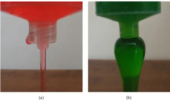
(26) Thèse de Himani Garg, Université de Lille, 2019. 8. Chapter 1. Visco-elastic fluids and elastic turbulence. Figure 1.1: Example of the Weissenberg effect with fluid climbing the rotating rod (picture from web.mit.edu). result, many of the theoretical polymer models proposed in the past 60 years have been verified and refined. Phenomenological models predicting the elasticity of macromolecules have been confirmed by many experiments [46]. Furthermore, much effort has been devoted to the detailed analysis of the motion of macromolecules in fluid flows [47]. Since the end of the 1940s it has been known that the addition of polymer additives to a fluid can drastically change its properties, and thus much effort has been devoted to the detailed analysis of the motion of macromolecules in fluid flows and to the rheological behaviour of the solution. Due to their molecular structure, polymers have elastic degrees of freedom which must be taken into account in the description of the mechanical response of the fluid to which they are added. Indeed, while for an ideal Newtonian fluid the stress is proportional to the deformation rate, the constant of proportionality being the viscosity, in an elastic material, the stress is proportional to the deformation itself, the constant of proportionality being the Hooke modulus. A solution of polymers in a Newtonian fluid can be thought of as a mixture of these idealized situations, because it presents characteristics of both viscous and elastic materials, and it is thus called a visco-elastic fluid. This structural difference in the dependence of the stress on the deforma-. © 2019 Tous droits réservés.. lilliad.univ-lille.fr.

(27) Thèse de Himani Garg, Université de Lille, 2019. 1.1. Polymer solutions. (a). 9. (b). Figure 1.2: (a) A Newtonian fluid is slowly extruded from a syringe. (b) The polymer solution which has been dyed green is slowly extruded from a syringe. On exiting, a noticeable swelling in the polymer solution stream several times larger than the diameter of the orifice is observed. Such a phenomenon is referred to as the Barus effect (Die swell) linked to non-zero normal stresses [48]. On the other hand, a Newtonian fluid does not exhibit the Barus effect. tion properties is the source of the distinctive behaviour of visco-elastic and Newtonian fluids. Among the large number of notable phenomena which are known to appear when dealing with visco-elastic fluids there is the rodclimbing (or Weissenberg) effect, the very large extrudate swelling at the exit of a die (as shown in Fig. 1.2), and many others (entanglement and turbulent drag reduction). Let us briefly consider the Weissenberg effect, also known as the rodclimbing effect [49] and the die swell effect [48]. Weissenberg effect: When a Newtonian fluid is placed in rotation, it is pushed away from the centre by the centrifugal force, and a dip appears on the free surface, which takes the shape of a paraboloid. In contrast, viscoelastic fluids tend to climb the rod [49]. Rod climbing is exhibited by liquids that show a normal stress difference (as shown in Fig. 1.1). In Newtonian liquids, the normal stresses (pressure) are isotropic even in flow, whereas. © 2019 Tous droits réservés.. lilliad.univ-lille.fr.

(28) Thèse de Himani Garg, Université de Lille, 2019. 10. Chapter 1. Visco-elastic fluids and elastic turbulence. polymeric liquids, upon the application of a shear flow, begin to develop normal stress differences between the flow and flow-gradient directions. Die swell effect: Analysing the motion of a fluid coming out from a capillary, a big difference can be observed between a Newtonian fluid and a visco-elastic fluid, as shown in Fig. 1.2. When a visco-elastic fluid flows out of a die, the diameter of the extrudate is usually greater than the size of the orifice. This is called die swell, extrudate swell, or the Barus effect [48] (as shown in Fig. 1.2). The degree of extrudate swell is generally of a difference between the diameter of the extrudate and the diameter of the die. For a fully developed flow of a visco-elastic fluid in a tube, there is tension along the streamlines. When the fluid exits the tube, it relaxes the tension along the streamlines by contracting in a longitudinal direction. For an incompressible liquid, this results in a lateral expansion, giving rise to the die-swell phenomenon. The effects produced by adding a polymer to a Newtonian fluid cover a wide range: they can modify the transport of heat, mass and momentum, influence the formation or depletion of vortices, and can change the stability of laminar motion and the transition to turbulence. A visco-elastic fluid can show a very interesting behaviour from a practical point of view, and a number of papers have been devoted to the understanding of the behaviour of visco-elastic fluids (see the references in [50]). The addition of a small amount of long-chain polymers to a Newtonian fluid flowing in a pipe can produce a dramatic reduction of the skin friction between the walls of the pipe and the fluid [51]. Drag reduction by polymer additives has been studied for more than half a century [52–54]. In this chapter, I will introduce the basics of polymer dynamics in fluids. Starting from a microscopic description in terms of the dynamics of a single polymer, the simple hydrodynamic models which have been typically used to describe visco-elastic solutions will be constructed. Further, I will briefly review the emergence of elasticity-driven turbulent-like states at small Reynolds numbers, which has been called elastic turbulence.. 1.2. The Weissenberg number. Since the end of the 1940s, it has been known that gradients of a velocity field can affect polymers and strongly deform them in fluid flow. A polymer in a fluid at rest typically resembles a spongy ball of size R0 , i.e. it. © 2019 Tous droits réservés.. lilliad.univ-lille.fr.

(29) Thèse de Himani Garg, Université de Lille, 2019. 1.2. The Weissenberg number. 11. Figure 1.3: Snapshots of single DNA molecule relaxing to a coiled state. In this experiment, a latex bead is tethered to an end of the molecule. The DNA molecule, coloured with a fluorescent dye, is stretched by a uniform flow and once the DNA molecule is fully elongated, the flow is turned off and the relaxation of the molecule is measured at different times [55]. is in a coiled configuration. In principle, all the configurations are permitted (even the fully stretched one) but in probabilistic terms, highly coiled configurations are much more probable. In contrast, when strong velocity gradients are imposed across a polymer, highly stretched states occur with large probabilities. The entropic tendency to return to a coiled state is indicated by an intrinsic parameter of the polymer, which is the time required by the molecule to reach the steady state in the absence of flow, starting from a non-coiled configuration. Polymer relaxation can be characterized by various measures of the relaxation time. Zimms’s time (relaxation time) is the largest of these. It depends on the temperature and viscosity of the solvent, on the number of monomers in the molecule, and on the effective length of the bonds between the monomers. The deformation of the polymer molecule is the result of the competition between the stretching exerted by the gradients of the velocity, and the relaxation of the polymer to its equilibrium configuration. Experiments with DNA molecules [55] have shown that this relaxation is linear, provided that the elongation is small compared to the maximum extension, i.e. R ≪ Rmax (see Fig. 1.3).. © 2019 Tous droits réservés.. lilliad.univ-lille.fr.

(30) Thèse de Himani Garg, Université de Lille, 2019. 12. Chapter 1. Visco-elastic fluids and elastic turbulence. Clearly the stretching rate of a given velocity field must be compared to the relaxation time of the molecule. If the velocity gradients are weak, then the restoring force predominates and the polymer molecule is not stretched. In contrast, if the stretching rates are very high the polymer molecules will be stretched. One should note that at least dimensionally, velocity gradients correspond to stretching rates. The whole concept of the relative strength of stretching with respect to relaxation can be quantified in terms of the non-dimensional Weissenberg number, named after the German physicist Karl Weissenberg: Wi =. τ τf. (1.1). where τf stands for the typical time scale of the flow and τ is the largest relaxation time [56]: τ=. µR03 kB T. (1.2). where kB is Boltzmann’s constant, T is the temperature, and µ is the dynamic viscosity of the solvent. When W i ≪ 1, the relaxation is fast, and thus a polymer stays in its coiled configuration. But W i ≫ 1 corresponds to an entirely stretchingdominated dynamics, and thus the polymers are substantially elongated. What happens for W i ≈ 1, i.e. when the relaxation and the stretching are competing with each other, is a natural question. Hinch and De Gennes were the first to address this question [57, 58], claiming that there is a sharp transition between stretching-dominated and relaxation-dominated states in strong flows, known as the coil stretch transition. A typical example cited by De Gennes where the transition is expected in the time-independent elongational flow. Chu and co-workers performed one of the first experiments where single-molecule measurements of the coil–stretch transition were taken in steady shear and elongational flows [59, 60]. There is also a coil–stretch transition for random flows [47], but the transition between the coiled and stretched configurations is not as sharp as in the elongational flows, because a random flow has a fluctuating extension rate, resulting in a broader distribution of polymer elongations. Many theoretical and numerical studies have also addressed the statistical nature of the polymer dynamics in random [61–63], simple shear or laminar [64–66], and turbulent flows [67–69].. © 2019 Tous droits réservés.. lilliad.univ-lille.fr.

(31) Thèse de Himani Garg, Université de Lille, 2019. 1.3. Visco-elastic models. 13. Figure 1.4: Dumbbell model. 1.3. Visco-elastic models. 1.3.1 The elastic dumbbell model A simplified model to represent the polymer molecule, which is often used, is the elastic dumbbell model. The model consists of a spring with elastic 3kB T constant H = 2R connecting a couple of beads of length b, negligible max b mass, and the same radius. Here Rmax is the maximum extension of the polymer molecule. Despite its simplicity, it can reproduce several rheological properties of dilute suspensions of polymers. The evolution of a dumbbell end-to-end separation vector R = x2 − x1 , where xi is the position of the bead, is characterized by the following forces: • the hydrodynamic drag force represents the drag experienced by the massless beads as they move through the solvent, • the Brownian force due to thermal fluctuations, • the elastic spring restoring force, which tends to bring the polymer molecule back to its equilibrium configuration. Moreover, assuming that in a homogeneous flow field the velocity gradients do not change appreciably over a distance comparable to the size of a massless bead, the evolution equation for R can be written as H R˙ = − R + Bξ β. © 2019 Tous droits réservés.. (1.3). lilliad.univ-lille.fr.

(32) Thèse de Himani Garg, Université de Lille, 2019. 14. Chapter 1. Visco-elastic fluids and elastic turbulence. where β is the friction coefficient and ξ is a zero-mean Brownian process modelling the Brownian forces with correlation < ξi (t)ξj (t′ ) >= δij δ(t − t′ ). √ 2R2. 0 depends on the average size of a polymer molecule The constant B = τ in its coiled state R0 and the relaxation time of the polymer τ , where. τ=. β . H. (1.4). If we assume that the flow field is inhomogeneous, it is reasonable to expect that polymers can also be stretched because of the differing velocities of the beads. Therefore, we must add an extra term R˙ = u(x2 , t) − u(x1 , t) to Eq. (1.3) to take into account the stretching due to the different velocities of the two beads. Here, u(x1 , t) and u(x2 , t) represent the velocities of beads at position x1 and x2 , respectively. Since the flow is smooth at the scale of the polymer, we can approximate this stretching term by the velocity gradient. The equation of motion of polymer can be rewritten as √ 1 2R02 R˙ = (R · ∇)u − R + ξ (1.5) τ τ This linear description of the dumbbell model is appropriate only for small elongations in the regime R ≪ Rmax . The description is no longer appropriate when the elongations develop to a great extent and become of the order of Rmax , because of the dependence of the friction coefficient β and the relaxation time τ on the elongation itself. Thus to take into account these effects, one of the possibile generalizations is to consider the Finite Extensible Non-Linear Elastic model (FENE model) [49]. This model assumes Rmax 2 −R2 τ → τR 2 2 . The friction coefficient β is estimated as β = 6πµR0 , which max −R 0. µR3. on plugging into Eq. (1.4) gives the Zimm relaxation time τ = kB T0 [56]. This unique characteristic time has to be seen as the largest relaxation time of the polymer dynamics. Higher oscillatory modes, with faster relaxation times, have been experimentally observed in DNA [70]. They can be only weekly excited by the gradients of the velocity in a turbulent flow. Thus in a simplified rheological model it is enough to keep only the principal mode, with the largest relaxation time.. 1.3.2. Hydrodynamic models. The previous description of the polymer dynamics accounts for the behaviour of a single polymer in a fluid, but does not take into account the back reaction of the polymers on the fluid. In order to take into account this. © 2019 Tous droits réservés.. lilliad.univ-lille.fr.

(33) Thèse de Himani Garg, Université de Lille, 2019. 1.3. Visco-elastic models. 15. feedback mechanism, it is necessary to move to a macroscopic hydrodynamic description. Several models have been introduced (see, e.g. [49, 71]). These models describe the fluid as non-Newtonian, taking into account the back reaction of the polymers on the flow by including an extra stress term in the momentum conservation equation. 1.3.2.1. The Oldroyd-B model. A model that is often adopted, due to its simplicity, is the linear viscoelastic Oldroyd-B model, which can be derived from the elastic dumbbell model [49]. The passage from the microscopic behaviour of a single molecule to a macroscopic description requires getting rid of the microscopic degrees of freedom, such as the thermal noise. The macroscopic dynamics of the polymer is conveniently described in terms of the conformation tensor ⟨Ri Rj ⟩ σij = (1.6) R02 where the average is taken over the thermal noise or, equivalently, over a small volume containing a large number of molecules. By definition, the conformation tensor σ is symmetric positive definite, and its trace tr (σ) is a measure of the elongation of the molecules of the polymer. The evolution equation for the conformation tensor σ can be derived from Eq. (1.5) (see Bird et al. 1987 [49]): σ−1 . (1.7) τ where τ is the polymer relaxation time defined in Eq. (1.4). It is important to remark that the matrix of the velocity gradient tensor has entries ∇u = ∂i uj . Here the conformation tensor σ is normalized by the equilibrium size R0 of the molecules, so that in the absence of an external fluid flow it relaxes to the unit tensor 1. Equation (1.7) must be supplemented by the evolution equation for the velocity field, which is derived from the momentum conservation law: ∂t σ + (u · ∇)σ = (∇u)T · σ + σ · (∇u) − 2. Dui 1 ∂Tij = + fi Dt ρf ∂xj. (1.8). where ρf is the density of the fluid, u is the velocity field, T is the stress tensor of the fluid and f is the sum of the body forces per unit mass. D The symbol Dt in Eq. (1.8) is known as the material derivative and is expressed as follows: Du ∂u = + u · ∇u (1.9) Dt ∂t. © 2019 Tous droits réservés.. lilliad.univ-lille.fr.

(34) Thèse de Himani Garg, Université de Lille, 2019. 16. Chapter 1. Visco-elastic fluids and elastic turbulence The total stress tensor of the fluid is given by T = TN + TP. (1.10). where T N is the viscous stress tensor and T P is an extra elastic stress tensor. The stress tensor in a Newtonian fluid is proportional to the rate of deformation, with constant of proportionality the viscosity of the fluid, and in the incompressible case, is usually expressed as TijN = −P δij + µ (∂j ui + ∂i uj ). (1.11). where µ is the dynamic viscosity of the solvent and P is the pressure. In the case of a visco-elastic solution, in the presence of polymers, the elastic stress tensor T P takes into account the elastic forces. In the Hookean approximation for the elasticity of the single polymer, the elastic stress tensor is proportional via the Hooke modulus to the deformation tensor T P = nHRi Rj . The elastic stress tensor per unit volume of fluid is obtained by summing the average contribution given by each polymer: T P = nH ⟨Ri Rj ⟩ = nHR02 σ. (1.12). where n is the concentration of polymer molecules. For an incompressible fluid of constant density ρf , substituting the expression for the elastic stress tensor into the momentum conservation law yields ∇p 2ηνs ∂t u + (u · ∇)u = − + νs ∆u + ∇·σ+f (1.13) ρf τ where νs = µ/ρ is the kinematic viscosity of the solvent and η is the zeroshear contribution of the polymers to the total viscosity of the solution ν = νs (1 + η): nHR02 τ η= 2µ Equation (1.7) together with Eq. (1.13) completely determines the dynamics of the Oldroyd-B model. 1.3.2.2. The FENE-P model. The Oldroyd-B model is based on the assumption that the molecules of the polymer can be modelled as Hookean springs, and consequently it allows for infinite extensions of the polymers. This is unphysical because the maximum length Rmax bounds the polymer end-to-end separation R. Moreover,. © 2019 Tous droits réservés.. lilliad.univ-lille.fr.

(35) Thèse de Himani Garg, Université de Lille, 2019. 1.3. Visco-elastic models. 17. the linear dumbbell model fails, and non-linearity becomes essential, when the polymer extension R approaches Rmax . A more refined, but still conceptually simple, description is that of the Finite Extensible Nonlinear Elastic model (FENE model), where the elastic constant H is replaced by the function 2 Rmax − R02 H(R ) = H 2 Rmax − R2 2. (1.14). diverging for R → Rmax , which means that the restoring force becomes infinite when the polymer is extremely stretched. Nevertheless, the introduction of non-linearities yields a non-linear evolution equation for the conformation tensor ⟨Ri Rj ⟩, which is not closed. A commonly accepted closure is the Peterlin approximation [72], consisting in a pre-averaging in the non-linear function: H(R2 ) = H. 2 Rmax − R02 2 Rmax − ⟨R2 ⟩. (1.15). This approximation leads to the following coupled equations for the velocity field u and the conformation tensor σ, in the FENE-P model: ∂t u + (u · ∇)u = −. ∇p 2ηνs + νs ∆u + H(tr(σ))∇ · σ + f ρf τ. ∂t σ + (u · ∇)σ = (∇u)T · σ + σ · (∇u) − 2. H(tr(σ))σ − 1 . τ. (1.16). (1.17). where the non-linear factor H(tr(σ)) is H(tr(σ)) =. trmax − tr(1) trmax − tr(σ). (1.18). 2 /R02 . with trmax = Rmax The FENE-P model is more accurate than the Oldroyd-B model in reproducing some of the features of polymer solutions, such as shear thinning, which are not included in the Oldroyd-B model. This model generally reproduces a more accurate scaling behaviour for the shear viscosity and the normal stress differences, and hence agrees well with the experimental measurements. Moreover, in numerical applications, the finite molecular extensibility reduces the onset of numerical instabilities due to the strong gradients of the conformation tensor field. For these reasons, this model is usually adopted in numerical simulations of visco-elastic channel flows [73–75].. © 2019 Tous droits réservés.. lilliad.univ-lille.fr.

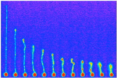
(36) Thèse de Himani Garg, Université de Lille, 2019. 18. 1.4 1.4.1. Chapter 1. Visco-elastic fluids and elastic turbulence. Elastic turbulence: An overview Experiments and theoretical investigations. One of the remarkable effects of polymers is that polymers with a long relaxation time τ and sufficiently high Weissenberg number W i are capable of giving rise to an irregular flow regime with velocity fluctuations spanning a broad range of spatial and temporal scales even in the limit of vanishing Reynolds number Re. The Reynolds number accounts for inertial instabilities and is defined by UL Re = (1.19) ν where U and L are, respectively, characteristic velocity and length scales and ν is the total viscosity of the solution. This irregular state caused by an instability due to the polymer stresses at high W i and in the limit of vanishing inertia, i.e. low Re, is known as elastic turbulence. The first quantitative experiments to demonstrate the onset of elastic turbulence were performed in a swirling visco-elastic flow of polymer solutions between two plates with a wide gap, in [21]. Steinberg and coworkers have identified a principal measure of elastic turbulence by measuring the ratio between the average shear stress and its corresponding value for a laminar flow between two rotating circular plates (see Ref. [21]). When the relative angular velocity between the two plates is increased, the average rescaled shear stress grows significantly, showing a sharp transition. The same maximum stress value is found in a corresponding flow of a Newtonian fluid for Re ∼ 104 , whereas the measurements were taken at Re < 1, showing that these effects are due to fluid elasticity. The frequency power spectrum of the velocity fluctuations in elastic turbulence displays a power-law decay, which spans about a decade in frequencies (see Fig. 1.5). The power-law dependence indicates that there is a broad range of timescales of the motion. It resembles that of the developed turbulence of a Newtonian fluid at high Re, but the energy spectrum has a steeper slope, i.e. the velocity fluctuations in elastic turbulence are concentrated at low wave numbers [8, 18, 21, 76]. This indicates that the flow is temporally irregular and driven by a few large scales. Qualitatively, the polymers are stretched by the shear flow, thus triggering purely elastic instabilities. These instabilities give rise to a secondary flow that acts back on the polymer molecules, stretching them further, and becomes increasingly turbulent, until a kind of saturated dynamic state is finally reached [18, 21, 23]. The fluctuating velocity field can be seen in the. © 2019 Tous droits réservés.. lilliad.univ-lille.fr.

(37) Thèse de Himani Garg, Université de Lille, 2019. 1.4. Elastic turbulence: An overview. 19. Figure 1.5: Power spectra of velocity fluctuations. The data were obtained at different shear rates ε. ˙ Curves 1 − 5 correspond to ε˙ = 1.25, 1.85, 2.7, 4 −1 and 5.9s , respectively. The spectrum of fluctuations is fitted by a power law, P ≈ f −3.5 , for ε˙ = 4s−1 . The figure is taken from the experiments of Groisman and Steinberg [21].. snapshots of the flow of the polymer solution above the transition, as shown in Fig. 1.6. The authors established that the onset of this new flow regime is due to a large elastic stress. Subsequently, a detailed experimental investigation was carried out by the same authors in three different systems: a shear flow between two circular plates, a Couette–Taylor flow, and a flow in a curvilinear channel (Dean flow) [25] (as shown in Fig. 1.7). The elastic turbulent flows are found to be highly correlated over space and the Eulerian temporal auto-correlation function decays rather fast with characteristic correlation times comparable to the largest polymer relaxation time [76]. Later, in 2006, a detailed experimental study of the previously unexplored transitional pathway from laminar to elastic turbulence provided a rich series of secondary flow states connecting the simple torsional shearing flow in a parallel plate device with elastic turbulence [77]. It has been found that the secondary-flow states involve axisymmetric rolls and non-axisymmetric spirals that compete at high Weissenberg number, producing oscillations,. © 2019 Tous droits réservés.. lilliad.univ-lille.fr.

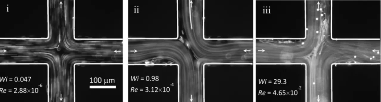
(38) Thèse de Himani Garg, Université de Lille, 2019. 20. Chapter 1. Visco-elastic fluids and elastic turbulence. Figure 1.6: Two representative snapshots of the polymer flows at W i = 13, Re = 0.7 taken from below. Figures are taken from the experiments of Groisman and Steinberg [21].. (a). (b). Figure 1.7: (a) Epifluorescent microphotograph of the entrance area of a microchannel used in experiments on mixing. Wide triangular region in front of a curvilinear channel allows adjusting equal flow rates for polymer solutions. (b) Confocal image of mixing in chaotic flow in the microchannel. Figures are taken from the experiments in a curvilinear micro-channel of a dilute solution of a high molecular weight polymer [18].. © 2019 Tous droits réservés.. lilliad.univ-lille.fr.

(39) Thèse de Himani Garg, Université de Lille, 2019. 1.4. Elastic turbulence: An overview. 21. (a). (b). Figure 1.8: Sample snapshots of dye advection experiments in straight microchannel system at Re < 0.01. (a) Newtonian case, (b) polymeric case, with W i = 10.9. The figure is taken from [26].. Figure 1.9: Flow patterns of visco-elastic fluid in the cross-slot geometry (i) Newtonian-like symmetric flow behaviour, (ii) steady asymmetric flow, and (iii) time-dependent flow. The figure is taken from [78].. apparent chaotic flow, and, eventually, apparent elastic turbulent flow with a broad spectrum of temporal fluctuations. The elastic turbulent flows are also characterized by divergent Lagrangian trajectories and, positive finite time Lyapunov exponents, could be measured by direct tracking of fluid particles in the flow and numerical integration of the measured flow velocity fields [23]. Systematic experiments performed in a von Karman flow between two disks by means of Laser Doppler Velocimetry and Digital Particle Image Velocimetry revealed a new characteristic space scale of the elastic turbulence, namely the width of the stress boundary layer [76]. A qualitative agreement with the theory of the elastic turbulence (discussed later) is found in terms of a saturation of the root mean square of fluctuations of the velocity gradients in the bulk of the flow [27].. © 2019 Tous droits réservés.. lilliad.univ-lille.fr.

(40) Thèse de Himani Garg, Université de Lille, 2019. 22. Chapter 1. Visco-elastic fluids and elastic turbulence. Since the pioneering work by Steinberg and coworkers, various microfluidic experiments have been performed to study elastic turbulence. In recent publications [18, 22, 27, 28, 79–82], it has been shown how these features of turbulence came into view in a highly elastic polymer solution at low Re in curvilinear flows, straight streamlines (as shown in Fig. 1.8), pipe flows and a cross-slot device (as shown in Fig. 1.9) [26, 78]. The behaviour of the flow observed for visco-elastic fluids is far more complex than that found for a Newtonian fluid. It is observed that visco-elasticity can lead to the onset of different types of purely elastic instabilities, depending on the rheological properties of the fluid. Other than in polymer solutions containing the usual high-molecular weight polymers (polyacrylamide, polyethylene oxide), the turbulent-like behaviour has also been perceived in complex fluids, in particular, using worm-like micelles for the elastic particles [83, 84]. The only existing theory of elastic turbulence in dilute polymer solutions with linear elasticity and the feedback reaction on the flow was published shortly after its discovery by Fouxon, Lebedev and Balkovsky [85, 86]. The major ingredient if the theory of the elastic turbulence is to relate the dynamics if the polymer stress tensor σ to the dynamics of a vector field with a linear damping [85–87]. The theory of elastic turbulence is restricted to unbounded flow of a polymer solution and is based upon the major assumption that the local feedback of the stretched polymer molecules on the flow field leads to a statistically stationary state by a saturation of both the polymer contribution to the stress tensor σ and the rms of the fluctuations of the velocity gradients (observed experimentally). With this assumption the theory explained the experimentally observed algebraic decay of the spectra of the velocity fluctuations and revealed the existence of an elastic turbulent regime. Latter a systematic description of these elastic instabilities (subcritical) in parallel shear flows of viscoelastic fluids is presented in Ref. [88]. Very recently a theory composed of a microscopic description of the polymer statistics and a macroscopic description of the stresses in a polymer solution has been proposed to investigate the boundary layer properties of elastic turbulence. Theory shows that in contrast to high Re , where the fluctuating velocity if always of the order of the mean flow in the viscous sublayer, wall-bounded elastic turbulence possesses a non-trivial relation between the mean and the fluctuating velocity components [89].. © 2019 Tous droits réservés.. lilliad.univ-lille.fr.

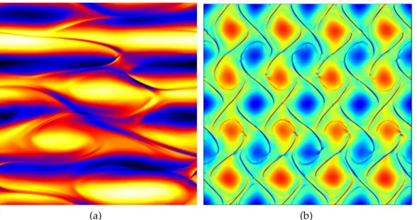
(41) Thèse de Himani Garg, Université de Lille, 2019. 1.4. Elastic turbulence: An overview. (a). 23. (b). Figure 1.10: Snapshot of vorticity field in numerical simulations of the twodimensional Oldroyd-B model (a) Re = 0.7 and W i = 22.4 and with a Kolmogorov forcing f = (F cos(y/L), 0), with L = 1/4 and where F = 64 is the forcing amplitude. The source of the figure is [90]; (b) Re = 1 and W i = 20 with a cellular forcing f = −F n [cos(nx) + cos(ny)] with n = 4 and F = 0.16 the forcing amplitude. The figure is taken from [91].. © 2019 Tous droits réservés.. lilliad.univ-lille.fr.

(42) Thèse de Himani Garg, Université de Lille, 2019. 24. 1.4.2. Chapter 1. Visco-elastic fluids and elastic turbulence. Numerical investigations. Elastic turbulence can also be numerically reproduced at least qualitatively in simulations using polymer solution models, for instance using the twodimensional Oldroyd-B model, in which only the largest relaxation time of the polymer is retained and the polymer elasticity is assumed to be linear. Preliminary attempts to simulate the elastic turbulence regime have been successful, for simplified 2D flow arrangements, such as the periodic Kolmogorov shear flow ( [90–93], Chapter 3). The Kolmogorov force produces a sinusoidal mean flow even in the presence of elastic polymers. Other constitutive models have been also used to simulate elastic tur-. (a). (b). Figure 1.11: (a) Contour plot of vorticity field for W i = 10 before and after the onset of a symmetry breaking transition. The study was performed by simulating the dynamics of the Oldroyd-B model, in a simple four-roll mill geometry [94]. (b) Snapshots of the normalized radial velocity component ur /umax for Weissenberg numbers of W i = 12.6, W i = 50.3 and W i = 106.8 (from left to right) in the 2D Taylor–Couette geometry. The figure is taken from [95]. bulence, such as those with a non-linear elastic force (FENE-P model), by. © 2019 Tous droits réservés.. lilliad.univ-lille.fr.

(43) Thèse de Himani Garg, Université de Lille, 2019. 1.4. Elastic turbulence: An overview. 25. taking into account the finite extensibility of polymers [96–98]. Numerical studies considering different flow geometries also display the presence of elastic instabilities [91, 94, 95] (see the snapshots of the vorticity field in Fig. 1.10(b) (cellular forcing), Fig. 1.11(a) (four-roll mill geometry) and Fig. 1.11(b) (2D Taylor-Couette geometry) ). Very recently, the occurrence of elastic turbulence of a visco-elastic fluid in a 2D Taylor–Couette geometry using the Oldroyd-B model has been investigated [95]. Numerical simulations show that for increasing fluid elasticity, i.e. increasing Weissenberg number W i, the Taylor–Couette or base flow becomes unstable. A secondary flow is created, which strongly fluctuates in time and which has a non-zero radial component. Snapshots of the normalized radial velocity component ur /umax are shown in Fig. 1.11(b). In fact, even a low-dimensional shell model of visco-elastic fluid reproduces elastic turbulence qualitatively [99]. Consistent with experimental results, numerical simulations indicate that the polymers stretch and apply stronger elastic forces to the flow if W i is sufficiently high. Numerically, it has been observed that the source of the turbulent stress comes from elasticity and elastic stresses play the role usually played by the Reynold stress in the usual inertial turbulence, which is the hallmark of elastic turbulence [90]. These experimental and subsequent numerical developments demonstrate that based on its similarity with turbulent fluid motion, elastic turbulence has been proposed as an efficient framework to enhance mixing in low Reynolds number flows [22]. The numerical investigation of elastic turbulence in two-dimensional Kolmogorov flows will be the subject of Chapter 3.. © 2019 Tous droits réservés.. lilliad.univ-lille.fr.


(45) Thèse de Himani Garg, Université de Lille, 2019. Chapter 2. Inertial particles in flows: Equations of motion and measurements of their concentration. Contents. 2.1. 2.1. Introduction . . . . . . . . . . . . . . . . . . . . . . . . . . . . .. 27. 2.2. The equations of motion for material particles transported by a flow . . . . . . . . . . . . . . . . . . . . . . . . . . . . . . .. 29. 2.2.1. Lagrangian tracer particles . . . . . . . . . . . . . . . .. 29. 2.2.2. Inertial particles . . . . . . . . . . . . . . . . . . . . . . .. 30. 2.3. The Stokes number . . . . . . . . . . . . . . . . . . . . . . . . .. 32. 2.4. The distribution of the particles in a flow . . . . . . . . . . .. 32. 2.4.1. The mechanism of preferential concentration . . . . . .. 33. 2.4.2. Correlation of preferential concentration with the fluid flow . . . . . . . . . . . . . . . . . . . . . . . . . . . . . .. 35. 2.4.3. Assessment of preferential concentration . . . . . . . .. 37. 2.4.4. Large scale clustering: Turbophoretic aggregation . . .. 42. Introduction. Particle-laden flows are everywhere, both in natural systems (sediments, plankton, aerosols, cloud droplets, etc.) and in human industrial activities (sprays, powders, combustion, extraction of oils, etc.). Predicting the dynamics of an ensemble of material particles transported in turbulent and non-turbulent flows remains a significant problem, which has motivated. © 2019 Tous droits réservés.. lilliad.univ-lille.fr.

(46) Thèse de Himani Garg, Université de Lille, 2019. 28. Chapter 2. Inertial particles in flows: Equations of motion and measurements of their concentration. countless studies over more than a century. Among the many situations where the transport of particles is of critical importance, a few environmental and industrial issues are worth being highlighted. For instance, the preferential concentration of inertial particles may enhance the probability of collision (and hence of coalescence) of water droplets in clouds, and therefore play an essential role in the initiation of rain [100, 101]. Similarly, it is believed that it can promote the agglomeration of fine particles in accretion disks, hence accelerating the formation of planetesimals [102]. In industrial applications, it can play a role in the coalescence of fuel droplets in diesel engines, and therefore affect the energetic efficiency, with significant economic and environmental implications [103]. The properties of particle suspensions are affected by the particle concentration as well as the by the properties of the suspending fluid. Indeed, variations of these characteristics induce important qualitative and quantitative changes in the behaviour of the suspension. It is intuitive that the scenario is even more complex when the suspending fluid itself has a complex rheological behaviour. Several industrial and daily-life materials fall in this category, including rubbers, detergents, paints, foods, and biological suspensions. The usual non-Newtonian properties, such as shear-thinning and the appearance of a normal stress difference, may strongly alter the micro-structure in flowing suspensions, even at low concentrations of particles. On the other hand, the peculiar particle dynamics induced by the complex rheology of the suspending fluid can be cleverly exploited to perform operations that would be difficult in Newtonian fluids. It is worthwhile to mention as an example the emerging use of non-Newtonian fluids in microfluidics to guide the suspended particles to some regions of the devices for counting, targeted drug delivery, diagnostics, the extraction of oils and gases from porous rocks, and particle separation applications [104]. Depending on the size and density of the particles relative to the fluid (eventually responsible for a non-zero response time of the particle due to its inertia), the particles will interact with the structures of the flow of the carrier at different time and spatial scales. Understanding the global dynamics of a particle suspended in Newtonian and non-Newtonian fluid flows is a topic of primary importance. This chapter is a review of some of the theoretical basis of the model equations which are currently employed to describe the motion of inertial particles under conditions of dilute suspension. This chapter also reviews the basic phenomenology of particle transport in turbulent flows, addressing, for instance, preferential concentration, and the tools currently used for. © 2019 Tous droits réservés.. lilliad.univ-lille.fr.

(47) Thèse de Himani Garg, Université de Lille, 2019. 2.2. The equations of motion for material particles transported by a flow 29. Figure 2.1: Visualization of turbulence by seeding the flow by 10 micron fluorescent polystyrene particles in a turbulent flow experiment (von Karman). The figure is taken from http://nicolas.mordant.free.fr/turbulence. html.. its quantitative characterization.. 2.2. The equations of motion for material particles transported by a flow. 2.2.1 Lagrangian tracer particles Fluid tracers are ideal particles which are transported by the flow without being subjected to any hydrodynamical or external force. Such particles, also called non-inertial tracers, are carried by the flow without having any effect on the flow field itself or on other quantities transported by the flow. Consequently, tracers can be thought of as identical to the fluid elements, and with the same density as that of the fluid (ρp = ρf ). These particles are ideally point-like and have the same velocity as the underlying fluid: dx = v(t) = u(x(t), t) dt. (2.1). where x and v are the position and velocity of tracer, respectively, and u is the velocity field of the fluid.. © 2019 Tous droits réservés.. lilliad.univ-lille.fr.

(48) Thèse de Himani Garg, Université de Lille, 2019. Chapter 2. Inertial particles in flows: Equations of motion and measurements of their concentration. 30. 2.2.2. Inertial particles. Unlike these fluid tracers, particles with a mass density that has a mismatch with that of the fluid (ρp ̸= ρf ) (either smaller, e.g. bubbles, or greater, e.g. sand grains) or with a size comparable to the characteristic scales of the flow (such as its smallest eddies) do not follow the flow exactly. Such particles are generally referred to as inertial particles. Particles with a density much greater than the density of the carrier fluid (ρp ≫ ρf ) are known as heavy inertial particles. In this thesis we only study heavy inertial particles. The formulation of the problem can be given in the following terms: considering a rigid sphere (density ρp and radius a) in a viscous Newtonian flow governed by the Navier–Stokes equations, with no-slip boundary conditions on the surface of the sphere, can we formalize the instantaneous action of the flow on the sphere? An answer to this longstanding question was formulated successively by Stokes [105] and Basset [106], and later refined by Boussinesq [107] and Oseen [108], who examined the motion of a sphere settling under gravity in a fluid at rest. Their analysis started from the unsteady situation of a sphere settling from rest in a quiescent viscous fluid, which concerns the transient acceleration until it reaches its terminal settling velocity. The difficulties encountered in this problem are independent of the dynamical regime of the fluid flow. The disturbance flow produced by the motion of the sphere was considered to have a sufficiently low Reynolds number (Rep ≪ 1) so that the fluid force on the sphere could be estimated from a Stokes flow (so that a second Reynolds number based on the spatial scale of shear is also small (ReS < 1)). Tchen extended this work to a sphere settling under gravity in a non-uniform flow, with a view already to turbulent flows [109]. The resulting model (known as BBOT, Basset–Boussinesq–Oseen–Tchen) was revised in 1983 and proper account taken of the Faxen correction for the unsteady Stokes flow, simultaneously by Maxey and Riley [110] and Gatignol [111], leading to the following equation of motion for a particle in a flow: mp. 1 d(u − v) Du dv = 6πµa(u − v) + mf + mf + (mp − mf )g+ dt 2 dt ∫ Dt t d(u − v) dt∗ √ √ 6a2 πρf µ dt t − t∗ −∞. (2.2). where v is the velocity of the particle, u is the velocity field of the unperturbed flow of the carrier, a is the radius of the particle, mp is the mass of the particle, ρf is the density of the carrier fluid, mf is the mass of the fluid displaced by the particle, and µ is the dynamic viscosity of the carrier fluid.. © 2019 Tous droits réservés.. lilliad.univ-lille.fr.