HAL Id: hal-02636673
https://hal.archives-ouvertes.fr/hal-02636673
Submitted on 26 Aug 2020HAL is a multi-disciplinary open access archive for the deposit and dissemination of sci-entific research documents, whether they are pub-lished or not. The documents may come from teaching and research institutions in France or abroad, or from public or private research centers.
L’archive ouverte pluridisciplinaire HAL, est destinée au dépôt et à la diffusion de documents scientifiques de niveau recherche, publiés ou non, émanant des établissements d’enseignement et de recherche français ou étrangers, des laboratoires publics ou privés.
New mixed integer approach to solve a multi-level
capacitated disassembly lot-sizing problem with
defective items and backlogging
Ilhem Slama, Oussama Ben-Ammar, Alexandre Dolgui, Faouzi Masmoudi
To cite this version:
Ilhem Slama, Oussama Ben-Ammar, Alexandre Dolgui, Faouzi Masmoudi. New mixed integer ap-proach to solve a multi-level capacitated disassembly lot-sizing problem with defective items and back-logging. Journal of Manufacturing Systems, Elsevier, 2020, 56, pp.50-57. �10.1016/j.jmsy.2020.05.002�. �hal-02636673�
Ilhem Slama, Oussama Ben-Ammar, Alexandre Dolgui, Faouzi Masmoudi. New mixed integer approach to solve a multi-level capacitated disassembly lot-sizing problem with defective items and backlogging.
Journal of Manufacturing Systems, Elsevier, 2020, 56, pp.50-57. ⟨10.1016/j.jmsy.2020.05.002⟩.
Mixed integer program to solve a capacitated disassembly scheduling
problem with lost and backordered items
Ilhem Slama1,2, Oussama Ben-Ammar1, Faouzi Masmoudi3, Alexandre Dolgui 1
1IMT Atlantique, LS2N, UMR-CNRS 6004, La Chantrerie, 4 rue Alfred Kastler - B.P. 20722, 44307 Nantes, France
2Laboratory of Modeling and Optimization for Decisional, Industrial and Logistic Systems (MODILS). Faculty of Economics and Management Sciences of Sfax, University of Sfax, Airport Road km 4, BP
1088, Sfax 3018, Tunisia
3Engineering School of Sfax, Laboratory of Mechanic, Modeling and Production (LA2MP), University of Sfax, Tunisia
E-mail : [email protected]; {ilhem.slama, oussama.ben-amma, alexandre.dolgui}@imt-atlantique.fr
Abstract
In the last few years, there has been a growing interest in the disassembly scheduling problem to fulfill the demands of individual disassembled parts over a given planning horizon. Planners have to determine the timing and the optimal quantity of ordering the end-of-life products. This paper focuses on the case of a multi-period planning problem, a single product type and multi-level structure. In this paper, we suggest a new mixed integer linear programming model for solving the capacitated disassembly scheduling problem in order to maximize total profit while minimizing of the sum of setup, inventory holding, external procurement, disposal, backlogging and overload costs in each time period. In other words, the objective function aims to (i) maximize the profit obtained by the resale of the recovered components after disassembly, from the valuation of the end-of-life products, and (ii) to minimize the costs related to the operation of disassembly process. Our computational experiments show that the proposed model gives the optimal solutions for all the test instances within acceptable time. Sensitivity studies on capacity, procurement and sale costs are also conducted, which provide some useful insights for industrial makers.
Keywords: Reverse logistic, Disassembly, Capacitated disassembly scheduling, Disposed items,
Backordering, Extra capacity.
1 Introduction
In the past decade, environmental protection has received growing attention. For economic, environmental and legislative reasons, waste reduction and recovery of end-of-life products have
become a major preoccupation (Benaissa et al. 2018). Reverse logistics, as the name suggests, refers to the logistics activities of an organization but in a reverse direction to what it may be in forward logistics. Their activities aim to plan collection, disassembly, repair, recycling, disposal, etc. of end-life products (Kim et al. 2018).
This research focuses on disassembly, which is one of the essential activities for recovering and elimination of used products in reverse logistics. In other words, the disassembly is one of the important domains in reverse logistics, since the end-of-life products cannot be recovered or even disposed of without disassembling them (Kim et al. 2018).
According to the classifications discussed by (Kim et al. 2018), the disassembly process necessitate to solve six categories of problems: disassembly planning, disassembly sequencing, disassembly line balancing, design of disassembly to order system, ergonomics and automation of disassembly systems. Among the disassembly problems mentioned earlier, our paper is based on R-MRP (Reverse-Material Requirements Planning) taking into account end-of-life products recovery process. R-MRP tends to be a disassembly planning system to determine when and how much end-of- life products to disassemble (Lee and Xirouchakis 2004). The goal is to meet customer components requirements over the planning horizon while minimizing the costs associated with the disassembly process.
Therefore, the following two questions are asked to optimize given performance indicators: (i) when to disassemble the end-of-life products? and (ii) how much end-of-life products must be disassembled to cover the demand for items used?
The literature on disassembly planning provides answers to these questions and offers a variety of approaches to help decision makers manage problems and improve their decisions in an unstable environment. (Lambert and Gupta 2004) highlighted that “a breakthrough in this domain came by considering the assembly process as a reverse of disassembly, which is valid under some specific assumptions”. (Kim and Xirouchakis 2010) argued the same point but went further to state that the disassembly planning problem can be regarded as a reverse version of the lot sizing problem for assembly systems. Authors indicated that, compared to assembly process, disassembly process is characterized by more different and complex physical and operational properties. In fact, the disassembly is a divergent process where a product is broken down into several parts and subassemblies, unlike the assembly where several parts converge to a single product. Due to divergence properties, the disassembly planning is more complex than lot sizing problem in the assembly systems. For more details of the divergence characteristics, readers can
refer to (Kim et al. 2007), or to (Morgan and Gagnon 2013), (Gagnon and Morgan 2014) and (Lee et al. 2001) for comprehensive reviews.
The main contributions of this paper include:
(1) A new compact and effective mixed-integer linear programming model (MIP) for the disassembly planning is suggested.
(2) In order to get close to reality as much as possible, we extend existing models to include additional parameters such as external procurement, disposed and backordered of items, setup time and extra capacity. These parameters make the problem more complex to handle mathematically. To the best of our knowledge, it is the first time to consider these parameters simultaneously.
(3) Some interesting managerial insights are observed. For example, increasing the disassembly capacity increase the quantities resulting from the disassembly. Moreover, small disassembly capacities extremely worsen the situation. They cause loss in profit. Therefore, managers should pay more attention to decreasing profit margin and procurement cost.
This paper is organized as follows. In the next section, we present a literature review on the relevant researches dealing with the disassembly planning problems. The studied problem is described in Section 3. Different mathematical programming models have been applied for disassembly planning with different objective functions. A new mathematical model is presented in Section 4. Numerical results are reported in Section 5. Finally, conclusions are drawn, and future studies are given in Section 6.
2 Related publications
This section reviews the previous studies on disassembly planning problems. Table 1 shows a summary of the relevant papers including our new approach. The classification is done according to two/multi levels structure, single/multi items, one/multi periods, commonality/no commonality of parts, capacitated/incapacitated constraints, and deterministic or stochastic approaches. In the next subsections, we review literature on approaches employed to model deterministic or stochastic, capacitated or incapacitated problems.
2.1 Deterministic and incapacitated models
Most of the earlier studies consider the deterministic incapacitated disassembly planning problems. To our knowledge, the first model was proposed by (Gupta and Taleb 1994) to study one-product type with multi-level structure and without parts commonality. They proposed a reverse material requirement planning algorithm (RMRP) without explicit objective function. Later, (Gupta et al. 1997) extended this basic case by considering the commonality of parts, and
suggested another RMRP algorithm to minimize the number of products to be disassembled. Parts commonality implies that a product or a sub-assembly shares its components and/or parts. (Taleb and Gupta 1997) considered the same problem but in the case of multiple types of products with parts commonality and suggested heuristics in two phases to optimize two independent objectives: to minimize the number of products to be disassembled and to minimize the total costs related to disassembly operations. (Kingdom 1998) proposed a mixed integer nonlinear program (MINLP) to maximize the profit and to satisfy the components demand by disassembling multi-products in each time period. Drawing on the work of (Taleb and Gupta 1997). (Neuendorf et al. 2001) proposed an algorithm based on Petri net that gives better solution than the reverse MRP algorithm. (Kim et al. 2003) derived the properties of the basic problem proposed by (Taleb and Gupta 1997) and applied in their work a heuristics algorithm and a linear programming (LP) relaxation approach to a case study to minimize the sum of setup, disassembly operation and inventory holding costs. (Lee and Xirouchakis 2004) derive the properties of the basic problem proposed by (Gupta and Taleb 1994) and suggested a two-phase heuristic in order to minimize the sum of purchase product, setup, disassembly operation and inventory holding costs. (Lee et al. 2004) proposed and solved three integer programming models for three problem cases, i.e. a single product type without parts commonality and single and multiple product types with parts commonality, they used CPLEX to solve the problem, the test results showed that the integer programming approaches can give optimal or near-optimal solutions only for small to medium size test problems. (Kim et al. 2006a) considered the disassembly planning problem with multiple product types and parts commonality and proposed a two-phase heuristic to minimize the sum of setup, disassembly operation and inventory holding costs. Later, (Langella 2007) presented an integer model and proposed a heuristic to solve a demand-driven disassembly planning problem with multiple product types, multi-levels product structure with the objective of minimizing the sum of separation, disposal, inventory holding and procurement costs. To solve this problem, they proposed a heuristic procedure that modifies the algorithm proposed by (Taleb and Gupta 1997) in order to alleviate the potential of infeasible solutions. (Gao and Chen 2008) proposed a genetic algorithm to solve the disassembly planning problem with a multi-level structure and one type product. The objective function is to minimize the sum of setup, inventory holding and disassembly operation costs. The results of computational experiments on randomly generated test problems indicate that the proposed approach gives the optimal solutions up to all moderate-sized problems in a short amount of computation time (less than 1 minute). (Kim et al. 2008) proposed a two-level disassembly structure and single type of product, to formulate the problem mathematically; they suggested an integer programming model and then reformulated
it into a dynamic programming model after having characterized properties of optimal solutions. (Barba-Gutiérrez et al. 2008) refocused attention on the use of MRP-like strategies proposed by (Gupta and Taleb 1994) and incorporated the lot sizing (LS-RMRP) to facilitate its use. Later, (Kim et al. 2009) proposed the Lagrangian relaxation-based heuristics with a branch and bound algorithm to address a multi-level and single-item disassembly planning problem without parts commonality.
Table 1. Summary on the literature review.
Authors Level Product PC C ap ac ity C riter ia Approach resolution Model type Two Mu lt i On e M u lt i De ter m in ist S to cha stic
Gupta and Taleb (1994) NP RMRP
Taleb et al. (1997) NP RMRP
Taleb and Gupta (1997) NP, 𝑑𝑐 Two phase Heuristics
(Kingdom 1998) Max profit MINLP
Neuendorf et al. (2001) NP Petri Nets
Lee et al. (2002) 𝑃𝐶, 𝐻𝑐,𝑑𝑐 LP
Kongar and Gupta (2002) Max profit, NPD Goal programming
Kim et al. (2003) 𝑆𝑐, 𝐻𝑐,𝑑𝑐 LP
Lee et al. (2004) 𝑆𝑐, 𝑃𝑐, 𝐻𝑐,𝑑𝑐 LP
Lee and Xirouchakis (2004) 𝑆𝑐, 𝑃𝑐, 𝐻𝑐,𝑑𝑐 Heuristics
Kim et al. (2005) NP Dynamic programming
Inderfurth and Langella (2005) 𝑑𝑐, 𝑍𝑐,𝑤𝑐 Heuristics
Kim et al. (2006a) 𝑆𝑐, 𝐻𝑐,𝑑𝑐 Two phase Heuristics
Kim et al. (2006b) 𝑆𝑐, 𝐻𝑐,𝑑𝑐 Lagrangian Heuristics
Kim et al.(2006c) NP Heuristics
Kongar and Gupta (2006) Max Profit, NPD Fuzzy goal programming
Langella (2007) 𝑆𝑐, 𝐻𝑐,𝑑𝑐, 𝑍𝑐,𝑤𝑐 Heuristics
Kim et al. (2008) 𝑆𝑐, 𝐻𝑐 Dynamic programming
Gao and Chen (2008) 𝑆𝑐, 𝐻𝑐,𝑑𝑐 Genetic algorithm
Barba-Gutiérrez et al. (2008) 𝑆𝑐, 𝐻𝑐,𝑑𝑐 LS-RMRP
Barba-Gutiérrez and
Adenso-Díaz (2009) NP F-RMRP
Kim et al. (2009) 𝑆𝑐, 𝐻𝑐, branch and bound
Kim and Xirouchakis(2010) 𝑆𝑐, 𝐻𝑐,𝑅𝑐 Lagrangian heuristics
Kang et al. (2011) 𝑆𝑐, 𝑑𝑐 Optimal algorithm
Kang et al. (2011) 𝑆𝑐, 𝑑𝑐 Heuristics
Kim and Lee (2011) 𝑆𝑐, 𝐻𝑐,𝑑𝑐 Heuristics
Prakashet al. (2012) 𝐻𝑐,𝑑𝑐 CBSA
Ullerich (2013) 𝑆𝑐, 𝐻𝑐,𝑑𝑐, 𝑍𝑐 Heuristics
Sung and Jeong (2014) 𝑆𝑐, 𝐻𝑐,𝑑𝑐, 𝑍𝑐 Heuristics
Ji et al. (2015) 𝑆𝑐, 𝐻𝑐,𝑑𝑐, 𝑍𝑐, 𝐶𝑐 Lagrangian heuristics Godichaud and Hrouga (2015) 𝑆𝑐, 𝐻𝑐,𝐿𝑐, 𝑂𝑐
Mixed Integer programming
(MIP), Genetic algorithm
Inderfurth et al. (2015) 𝑆
𝑐, 𝐻𝑐,𝑑𝑐, 𝑍𝑐,𝑤𝑐
Empirical and mathematical
analysis
Hrouga et al. (2016a) 𝑆𝑐, 𝐻𝑐,𝐿𝑐 GA and Fix and optimize
Hrouga et al. (2016b) 𝑆𝑐, 𝐻𝑐,𝐿𝑐, 𝑂𝑐 Heuristics
Liu and Zhang (2018) 𝑆𝑐, 𝐻𝑐,𝑃𝑐 Outer approximation
Kim and Lee (2018) 𝑆𝑐, 𝐻𝑐,𝑑𝑐 Two phase heuristics
Tian and Zhang (2018)
𝑆𝑐, 𝑃𝑐, 𝐻𝑐, 𝑤𝑐 PSO and dynamic programming
Current paper 𝑆𝑐, 𝐻𝑐,𝐴𝑐,𝑍𝑐,𝑂𝑐,𝑤𝑐,
Max Profit MILP
PC: Parts commonality, NP: Number of products to be disassembled, NPD: number of products to be disposed,𝑆𝑐: setup cost,𝑃𝑐: purchase cost of root,𝐻𝑐: Holding cost,𝑑𝑐:disassembly operation cost, 𝑍𝑐: purchase cost of parts,𝑊𝑐: disposal
cost,𝑅𝑐 : unsatisfied demand penalty cost, 𝐶𝑐: Start-up cost, 𝐿𝑐: lost sales penalty cost, 𝑂𝑐: overload cost, 𝐴𝑐:
Backlogging cost, CBSA: Constraint-Based Simulated Annealing Algorithm.
Unlike in the previous studies, (Kang et al. 2011) are the first to integrate the leveling and the disassembly planning problems at the same time. In this research, an optimal algorithm was proposed for the basic case problem with multiple products and single period and a heuristic for the extended problem with parts commonality after proving that the problem is NP-hard. (Kim and Lee 2011) extended the research result of (Kang et al. 2011) by considering a multi-period version. To solve this problem, they suggested a heuristics algorithm using a priority rule. Recently, (Kim et al. 2018) used the model suggested by (Kim and Lee 2011) and proposed a two-phase heuristic that consists: firstly, constructing an initial solution using a priority-based greedy heuristic and then improving it by removing unnecessary disassembly operations.
2.2 Stochastic and incapacitated models
Regarding the stochastic models, the authors generally consider uncertain parameters such as demands and yields. Considerations of uncertainties in the disassembly scheduling problem have not been addressed much in the literature. In fact, very few studies that dealt with the stochastic aspect have been published. To the best of our knowledge only three previous researches considered a non-deterministic incapacitated disassembly planning problem and they are confined to a single period planning. (Inderfurth and Langella 2006) consider multiple product types, parts commonality, two-level structures and yield uncertainty. A heuristic introduced to minimize the sum of disassembly operation, purchasing and disposal expected costs. By contrast,( Kongar and Gupta 2006) extends their earlier work (Kongar and Gupta 2002) by incorporating uncertainty in the number of end-of-life products retrieved, the total profit goal and the sum of recycled components. They utilized the fuzzy goal programming, which allow the goals of the problem to be characterized using intentional vagueness. (Barba-Gutiérrez and Adenso-Díaz 2009) extended the model proposed by (Barba-Gutiérrez et al. 2008) by integrating the uncertainty demand. For solving this problem, they proposed an algorithm F-RMRP (R-MRP based on a fuzzy logic).
2.3 Deterministic and capacitated models
There is a few of literature treats the capacitated disassembly planning problem. In fact, the capacity constraint makes the problem much more complex (Lee et al. 2002). The previous
researches on capacitated disassembly planning can be classified into single and multi-product structures.
For a single item, (Lee et al. 2002) are the first to study a deterministic capacitated problem.
They suggested an integer programming model to minimize the sum of disassembly operation, purchase products and inventory holding costs. For the same problem, (Kim et al. 2005) minimize the number of disassembled products and suggested an optimization algorithm. Authors prove that its optimal solution value is equal to the one found in an incapacitated problem. Then, (Kim et al. 2006b) extended the research result of , (Kim et al. 2005) by adding setup, disassembly operation and inventory holding costs in the objective function and proposed a Lagrangian heuristic algorithm. On the other hands, (Prakash et al. 2012) proposed a constraint-based simulated annealing algorithm to solve a single item disassembly planning problem with parts commonality.
For multiple items, (Ullerich and Buscher 2013) formulated a complete disassembly planning as
an integer linear programming model and considered a capacity constraint in each period. However, this work ignored the set-up cost which is a common and indispensable parameter in the industrial reality. On their part, (Ji et al. 2016) extended the work of (Ullerich and Buscher 2013) by introducing the start-up and the set-up costs and proposed a Lagrangian relaxation heuristic to address a capacitated disassembly planning with parts commonality. Another study was proposed by (Godichaud et al. 2016) to treat a capacitated lot-sizing disassembly problem with lost sales and penalty cost for overloading disassembly capacity, this problem was formulated as a MIP model and a GA was proposed to give a solution to this problem in a reasonable completion time for a large instance. In their study, (Hrouga et al. 2016a) combined a GA and Fix-and-Optimize heuristics to solve the multiple type products disassembly lot sizing problems with lost sales and capacity constraints. (Hrouga et al. 2016b) considered the disassembly lot sizing problem with lost sales, multi-product types, two levels and capacity constraint. To solve this problem, they proposed an efficient optimization method based on genetic algorithm and Fix-and-Optimize heuristics in order to minimize of the sum of setup, inventory holding, lost sales and overload costs. The last paper dealing with the studied problem has just been published by (Tian et Zhang 2018) in which the return of the returned products depends on the purchase price. The problem is formulated as a Nonconvex Mixed Integer ¨Program. The Particle Swarm Optimization (PSO) algorithm and dynamic programming are
combined to solve the problem in order to determine the correct acquisition prices of returned products, the appropriate timing and quantity of disassembly.
2.4 Stochastic and capacitated models
The existing literature on the stochastic capacitated disassembly planning problems is limited. Only three publications populate this category. (Kim and Xirouchakis 2010) considered the problem with multiple periods, multiple product types, two-level product structures, and stochastic demands. The objective is to minimize the sum of expected setup, inventory holding, and penalty costs on the non-satisfaction of requests. To solve this problem, they developed Lagrangian relaxation heuristics to solve it. (Inderfurth et al. 2015) formulated a disassembly planning problem, which stochastic yield, and suggested two-root and three-leaf mathematical model to illustrate the effect of yield uncertainty in stochastically proportional and binomial models respectively. In a recent paper by (Liu and Zhang 2018) a capacitated disassembly planning problem with random yields and demands is proposed. This problem is formulated as a mixed integer nonlinear program (MINLP) and an outer approximation-based solution algorithm is proposed to solve it.
In most studies, the authors considered that the disassembled items are all in a perfect condition besides and their state satisfies the demand. However, in the industrial reality, these items can be defective. Therefore, very few studies have studied the disassembly planning problem with the integration of disposal decisions. For this reason, it seems interesting for us to build a good example of the capacitated disassembly planning problem with certain specified demands for items, disposed items, external procurement, setup time, backordering and extra capacity. The relevant questions become how many roots should be disassembled in order to fulfill the demand in a cost-efficient manner. With only one item, the answer can be simply calculated and will be explained in the next section.
3 Problem description
3.1 Basic problem
This section will put forth a new mixed-integer linear program (MIP) model which can be used to obtain optimal solutions for a capacitated disassembly planning problem. We consider a problem with the disassembly product structure shown in Fig 1.
The disassembly structure with only one type of product must be explained first. The end-of-life product to be disassembled represents the root item, and the leaf items are the parts/components to be requested and not disassembled further. The parent element has more than one child and a child element denote item that has only one parent. Fig 1 shows an example of the disassembly structure, where element 1 designates the root item, items 2 and 3 represent the subassemblies items, and items 4-7 designate the parts or the leaf items. Similarly, the number in parentheses represents the number of units (yield) of the element obtained when a unit of its parent is disassembled; for example, item 2 is disassembled in three units of item 4 and one unit of item 5. Here, item 2 is called parent item, while items 4 and 5 are called child items. Also, the disassembly lead time denote by DLT implies the total time required to disassemble a parent item (Kim et al. 2006).
Fig 1. Disassembly structure: example
According to the disassembly structure described above, we consider the capacitated disassembly planning problem while satisfying the capacity over a planning horizon, that is to say, the total time required to perform the disassembly operations in each period must be less or equal than the available disassembly capacity in this period (Hrouga et al. 2016a) .
It is often too easy to impose a single capacity constraint over the planning horizon. This is because it is often the case that capacity can be added as would be the case if the disassembly plan called for it. Typical examples are the use of overtime or to bring in extra resources (VoB and Woodruff 2003). To keep our language simple, we refer to all these capacity additions such as overtime. Moreover, we assume that the capacity on overtime is limited.
The most researches on planning problem consider the setup cost in the objective function, that is to say when a parent item is disassembled, the equipment required for that item has to be set
DLT=1
up. This results in a set-up cost that is specific for each non-leaf item (can be root or subassemblies item). Although several previous researches on the capacitated disassembly planning problem do not consider the corresponding setup time required for preparing the disassembly operation. In general, the setup time is important, especially in manual disassembly operations, and hence should be integrated in the capacity constraint ( Kim et al. 2007). However, this issue increases the problem complexity more significantly. To the best of authors’ knowledge, no one has addressed the optimization of capacitated disassembly planning problem with setup time.
3.2 Problem statement and assumptions
In our model, the most goal is to fulfill the demand for items (can be subassemblies, or leaf items), which can either be seen as direct or external demand for non-root items (subassemblies and leaf items), or an internal demand for non-leaf items stemming from demand for remanufactured products and subassemblies items. All requirements must be satisfied either by disassembling the end of- life products, or we have assumed that we have access to new non-root items and can choose to buy these directly as a way to avoid disassembly with a very high penalty in the objective function. Inventory holding costs occur when are held in order to satisfy future demand.
The non-root items are also allowed to be disposed of at given costs and to be late with a penalty function may be used to model the fact that delay is a problem for some customers. Our concern is to make a simple model that allows non-root-items to be tardy but requires the end-of-life product to be on time. We assume that every unsatisfied demand on times is backordered. The disassembly planning problem considered in this paper can be defined as the problem of determining the disassembly plans of all parent items for a given disassembly product structure, while satisfying the external demand of non-root item over a certain planning horizon with the objective of maximizing the profit obtained by the resale of the recovered components after disassembly while minimizing the sum of setup, inventory holding, purchase, disposal, backlogging and overload costs over the planning horizon.
Given a deterministic demand for non-root items, a product structure, and the above-described relevant costs, this work concentrates on answering the following questions:
When should be disassembled the parent items, how much of each non-root item should be purchased, stored, backordered, sold, or disposed of, and how much of extra capacity can be added over a given planning horizon in order to meet this demand?
The conceptual model for the studied problem is presented by a mass flow diagram in Fig 2.
Fig2. Mass flow diagram of decision environment
The assumptions can be summarized as follows:
- The demands of the components are given and deterministic.
- The demand can be satisfied with the disassembly operation and/or the external procurement. - The backlogging is allowed; hence the demand may not be satisfied on time.
- The initial inventory of the items is assumed to be zero.
- The items obtained may not all be in good condition to meet the demand.
- There is no storage for the end-of-life products that can be obtained once they are requested. - Disassembly operation time and setup time of all parent items and deterministic.
- The capacity on overtime disassembly is limited. - The cost parameters are assumed to be constant.
4 New problem formulation
This paper presents the optimization of an R-MRP model. The objective is to find the optimal used/end-of-life products to satisfy customer demands on a given delivery date. To formulate this problem, all items in the disassembly structure are numbered in the topological order from bottom to top and from left to right, starting with number one for the root item. In our model, without loss of generality, all items are numbered by integers: 1,2, … . , 𝑖𝑙, 𝑖𝑙+1… , 𝑃 where 𝑖𝑙+1 denote the index for the first leaf item. Hence, all indices that are larger than 𝑖𝑙 represent leaf items.
Disassembly planning
Items from disassembly operation
Items from stock
Items externally purchased
Items stored for future demand
Items consumed by costumers Items disposed of
In order to suggest a new problem formulation, the idea is to compact the inventory balance equations for the parent items and the one for each leaf item as it is proposed in the literature in a single inventory equation. Indeed, we have inspired the idea from the mathematical formulation of MRP (Material Requirements Planning) production planning problem proposed by (VoB and Woodruff 2003) and we have adopted it in a R-MRP model , since the problem is basically a reversed form of the regular MRP (Lee et al. 2001).
Let 𝑖 = 1 be the index of the end-of-life product and 𝑃 the index of the last item obtained by disassembling it. Let the following three sets: (i) ℰ the set of items 𝑖 with 𝑖 = 1, … , 𝑃, (ii) 𝒜 the set of items 𝑖 of the last level of product structure which cannot be disassembled. These items verify the following equality: ∀ 𝑖 ∈ 𝒜, ∀𝑗 ∈ ℰ| 𝑅(𝑖, 𝑗) = 0, and (iii) 𝒜𝐶 the set of remaining items such as 𝒜 ∪ 𝒜C= ℰ. To facilitate model reading, we introduce a macro, denoted by ≡ to indicate the inventory of an item 𝑖 in each time period 𝑡.
The full list notations used throughout this paper is given below:
Indexes
𝑖 index for items 𝑖 = 1,2, . . . , 𝑃 𝑡 index for periods 𝑡 = 1,2, … … . , 𝑇
Parameters
𝑃 Number of items 𝑇 Number of time buckets
ℰ Set of items 𝑖 with 𝑖 = 1,2, . . . , 𝑃
𝒜𝐶 Set of items 𝑖 such as 𝒜 ∪ 𝒜𝐶 = ℰ (non-leaf items)
𝒜 Set of items 𝑖 of the last level of the product structure (leaf items)
𝑅(𝑖, 𝑗) number of units (yield) of item 𝑗 obtained from disassembling one unit of item 𝑖(𝑖 < 𝑗) 𝐷(𝑖, 𝑡) External demand of item 𝑖 (part or subassembly) in period 𝑡
𝐼(𝑖, 0) Beginning inventory of item 𝑖 𝐷𝐿𝑇(𝑖) Disassembly lead time of item 𝑖
𝐻(𝑖) Per period inventory holding cost of one unit of item 𝑖 𝑆(𝑖) Per period set-up cost of parent item 𝑖
𝜑(𝑖) parent of item 𝑖
𝐴(𝑖) Per period backlogging costs of one unit item 𝑖 𝐶(𝑖) Unit purchasing cost of one unit item 𝑖
𝛼(𝑖, 𝑡) Waste rate of item 𝑖 in period 𝑡 𝐺(𝑖) Disassembly operation time of item 𝑖 𝑈(𝑡) Disassembly capacity in time, in period 𝑡 𝑂(𝑡) Penalty cost disassembly time in period 𝑡
𝐹(𝑡) Disassembly capacity on overtime in time, in period 𝑡 𝐸(𝑖) Per period disposal cost of one unit item 𝑖
𝑆𝐶(𝑖) Per period sale’s cost of item 𝑖 𝑆𝑇(𝑖) Setup time of item 𝑖
𝑀 A large number
Decision variables
𝑥𝑖𝑡 Order release quantity of item 𝑖 in period 𝑡, ∀ 𝑖 ∈ 𝒜𝐶
𝛿𝑖𝑡 Binary indicator of disassembly of item 𝑖 in period 𝑡, ∀ 𝑖 ∈ 𝒜𝐶 𝐼𝑖,𝑡+ Inventory level of item 𝑖 at the end of period t ∀ 𝑖 ∈ ℰ∖{1} 𝐼𝑖,𝑡− Backordered quantity of item 𝑖 in period t ∀𝑖 ∈ ℰ∖{1} 𝑧𝑖𝑡 Procurement quantity of item 𝑖 in period t ∀𝑖 ∈ ℰ∖{1} 𝑤𝑖𝑡 Disposal quantity of waste of item i in period t ∀ i ∈ ℰ∖{1} 𝑦𝑡 Disassembly “Overtime” in period 𝑡
𝑄𝑖𝑡 Sale quantity of item 𝑖 in period t ∀ 𝑖 ∈ ℰ∖{1}
The optimization model is as follows. The objective function (1) maximizes the total sale cost while minimizing of the sum of inventory holding, backlogging, external procurement, disposal, setup, and overload costs over the planning horizon.
𝑀𝑎𝑥 ∑ (∑(𝑆𝐶(𝑖). 𝑄𝑖𝑡− 𝐻(𝑖). 𝐼𝑖,𝑡+ − 𝐴(𝑖). 𝐼𝑖,𝑡− − 𝐶(𝑖). 𝑧𝑖𝑡 − 𝐸(𝑖). 𝑤𝑖𝑡) 𝑃 𝑖=2 − 𝑂(𝑡). 𝑦𝑡 𝑇 𝑡=1 − ∑ 𝑆(𝑖). 𝛿𝑖𝑡 𝑖∈𝒜𝐶 ) (1)
Eq. (2) represents the demand and materials requirement for all non-root item 𝑖 and period 𝑡: In other words, at the end of the planning horizon, all requests of non-root item 𝑖 must be satisfied
𝐼𝑖,𝑡(𝑥) + ∑ 𝐷(𝑖, 𝜏) ≥ 0 𝑡
𝜏=1
∀ 𝑖 ∈ ℰ∖{1} ; ∀ t = 1, . . , 𝑇 (2)
Where 𝐼𝑖,𝑡(𝑥) the macro defined as follows:
𝐼𝑖,𝑡(𝑥) ≡ ∑ ∑(𝑅(𝜑(𝑖), 𝑖). 𝑥𝜑(𝑖),𝜏) 𝑃 𝑖=2 + 𝐼(𝑖, 0) − ∑(𝐷(𝑖, 𝜏) + 𝑥𝑖,𝜏+ 𝑤𝑖,𝜏− 𝑧𝑖𝜏) 𝑡 𝜏=1 𝑡−𝐷𝐿𝑇[𝜑(𝑖)] 𝜏=1
Eq. (3) defines the inventory balance for each non-root item 𝑖 at the end in each period 𝑡:
𝐼𝑖,𝑡+ − 𝐼𝑖,𝑡− = 𝐼𝑖,𝑡(𝑥) ∀ 𝑖 ∈ ℰ∖{1}, ∀ 𝑡 = 1, . . , 𝑇 (3)
Eq. (4) represents the modeling constraint for disassembly indicator for each non-leaf item 𝑖 and period 𝑡:
𝛿𝑖𝑡−𝑥𝑖,𝑡
𝑀 ≥ 0 ∀ 𝑖 ∈𝒜
𝐶, ∀ 𝑡 = 1, . . , 𝑇 (4)
Eq. (5) represents the waste quantity for each non-root items 𝑖 and period 𝑡:
w𝑖𝑡 = 𝛼(𝑖, 𝑡). 𝑅(𝜑(𝑖), 𝑖). 𝑥𝜑(𝑖),𝑡−𝐷𝐿𝑇[𝜑(𝑖)] ∀ 𝑖 ∈ ℰ∖{1}, ∀ 𝑡 = 1, . . , 𝑇 (5)
Eq. (6) represents the capacity constraint in each period 𝑡: ∑ (𝑆𝑇(𝑖).𝛿𝑖𝑡+ 𝐺(𝑖)
𝑖∈𝒜𝐶
. 𝑥𝑖,𝑡) ≤ 𝑈(𝑡) + 𝑦𝑡 ∀ 𝑡 = 1, . . , 𝑇 (6)
Eq. (7) represents the disassembly capacity on overtime in each period 𝑡:
𝑦𝑡 ≤ 𝐹(𝑡) ∀ 𝑡 = 1, . . , 𝑇 (7)
Eq. (8) guarantees that the backordered quantity for each item 𝑖 and period 𝑡 should be less than or equal to the demand in that period 𝑡:
Eq. (9) ensures that any quantity externally purchased of each item 𝑖 and period 𝑡 cannot exceed the demand in that period 𝑡:
𝑧𝑖𝑡 ≤ 𝐷(i, 𝑡) ∀ 𝑖 ∈ ℰ∖{1}, ∀ 𝑡 = 1, . . , 𝑇 (9)
Eq. (10) represents the sale quantity for each non-root item 𝑖 and period 𝑡:
𝑄𝑖𝑡 = (𝐷(i, 𝑡)−𝑧𝑖𝑡) ∀ 𝑖 ∈ ℰ∖{1}, ∀ 𝑡 = 1, . . , 𝑇 (10)
Eq. (11) – (19) provides the conditions on the decision variables:
𝑤𝑖,𝑡≥ 0 ∀ 𝑖 ∈ ℰ∖{1}, ∀ 𝑡 = 1, . . , 𝑇 (11) 𝑦𝑡 ≥ 0 ∀ 𝑡 = 1, . . , 𝑇 (12) 𝐼𝑖,𝑡− ≥ 0 ∀ 𝑖 ∈ ℰ∖{1}, ∀ 𝑡 = 1, . . , 𝑇 (13) 𝐼𝑖,𝑡+ ≥ 0 ∀ 𝑖 ∈ ℰ∖{1}, ∀ 𝑡 = 1, . . , 𝑇 (14) 𝑧𝑖𝑡 ≥ 0 ∀ 𝑖 ∈ ℰ∖{1}, ∀ 𝑡 = 1, . . , 𝑇 (15) 𝑥𝑖,𝑡 ≥ 0 ∀ 𝑖 ∈ 𝒜𝐶, ∀ 𝑡 = 1, . . , 𝑇 (16) 𝑥𝑖,𝑡 ≤ 0 ∀ 𝑖 ∈ 𝒜, ∀ 𝑡 = 1, . . , 𝑇 (17) 𝑄𝑖,𝑡 ≥ 0 ∀ 𝑖 ∈ ℰ∖{1}, ∀ 𝑡 = 1, . . , 𝑇 (18) 𝛿𝑖,𝑡∈ {0,1} ∀ 𝑖 ∈ 𝒜𝐶, ∀ 𝑡 = 1, . . , 𝑇 (19) 5 Numerical results
The CPLEX 12.6 commercial software package was used to solve optimally the new mixed integer linear programming (MILP). In fact, the program which generates the MILP formulations was coded in C with an Intel (R) Core ™ i7-5500 CPU @ 2.4 GHz.
5.1 Sensibility analysis
Sensitivity analysis is generated on a small instance on the product structure shown in Fig 1, when T = 10, P = 7. We conduct sensitivity study on three main parameters of the problem, namely disassembly capacity, sale and procurement costs. All these tests are carried out under parameters costs generated in table 2. The demand of non-root items is generated from the discrete uniform distribution 𝐷~𝑈(0,100) over the planning horizon. The units inventory holding, disposal, setup, and penalty disassembly time costs are generated from the discrete uniform distribution with [a, b]. For each non-root item, the unit backlogging cost 𝐴(𝑖) is
assumed twice as large as the unit inventory holding cost. The waste rate 𝛼(𝑖, 𝑡), for item 𝑖 ∀ 𝑖 ∈ ℰ∖{1}, is generated according to 𝐷~𝑈 (0,10). We assume that each disassembly operation time 𝐺(𝑖) and setup time 𝑆𝑇(𝑖) are 𝐷~𝑈(1,4) and 𝐷~𝑈(10,20), respectively for all 𝑖 ∈ 𝒜𝐶. The total disassembly capacity, 𝑈(𝑡) and disassembly capacity on overtime, 𝐹(𝑡) are generated according to 𝐷~𝑈 (240,480), 𝐷~𝑈 (60,120), respectively.
According to the real-life case, we assume that the costs of purchase new items are greater in front the unit cost of disassembling (setup and holding costs) and disposal of items issued from the disassembly process. Two parameters γ, β ∈ ℝ+ are introduced to fix the units sale and purchase costs, where 𝛾 and β represent the profit margin and margin compared to cost generated by the disassembly process, respectively. It has been assumed in this example that 𝛾 to 1.5 and β to 1.8.
Table 2: Values costs generation Parameters Value 𝐻(𝑖) 𝐷~𝑈 (12,20) 𝑆(𝑖) 𝐷~𝑈 (0,1500) 𝐴(𝑖) 2 × 𝐻(𝑖) 𝐸(𝑖) 𝐷~𝑈 (15,30) 𝑂(𝑡) 𝐷~𝑈 (20,25) 𝑆𝐶(𝑖) γ × (𝐻(𝑖) + 𝑆(𝑖) + 𝐸(𝑖)) 𝐶(𝑖) 𝛽 × (𝐻(𝑖) + 𝑆(𝑖) + 𝐸(𝑖))
Impact of capacity time
The total costs composition in table 3 shows that larger capacity leads to larger total cost. In fact, larger capacity is preferred in terms of operational costs (larger sales and smaller external procurement as shown in Fig 3). A few capacities limit the productivity within a minimum disassembly quantity, larger overload and external procurement costs.
Table 3: Impact of capacity time on the total cost and cost items
𝑼 Total cost Sale cost Procurement cost Holding cost Backlogging cost Setup cost Overload cost 240 151361.203 185759 6075 2757 3690 2900 18975 320 166022.906 186417 5285 3831 3778 2700 4800 400 175416.703 189577 1495 4273 5392 3000 0 480 176027.297 190135 825 4664 5618 3000 0
However, when capacity is relatively small, managers have no alternative but to satisfy a part of the requirements by external procurements. Extremely, excessively small capacity and small
extra capacity causes infeasibility. However, managers should also balance the trade-off between higher capacity investment, lower operational costs and larger of sales.
Fig 3: Disassembly quantity under different capacity value
Impact of procurement cost
To know until which cost of purchase it is profitable to satisfy the demands of components by disassembling the end-of-life products, we fix the profit margin 𝛾 to 1.5 and we vary the ratio 𝛾 𝛽⁄ between 10−3 and 103. Then, the quantities resulting from the disassembly and the external purchases to satisfy the external demands as function of the ratio 𝛾 𝛽⁄ are obtained in Fig 4.
Table 4: Impact of procurement cost on the total cost and cost items
𝛾 𝛽⁄ Total cost Sale cost Procurement cost Holding cost Backlogging cost Setup cost Overload cost 10−3 560320.563 1217587 586498 11583 12584 22000 24600 10−2 1082298.000 1217555 61800 14088 12670 21999 23680 10−1 1119148.000 1215053 31200 10943 8638 23000 22125 1 1157070.000 1211201 6971 3448 5612 24000 14100 10 1164231.375 1197201 2095 4951 6498 18000 1425 10 2 1169190.125 1197934 201 6256 6586 10000 700 10 3 1164578.875 1198088 17 8636 5904 17000 700
Economically speaking, to satisfy the external demand, the quantity from disassembly operation decreases as function of the ratio 𝛾 𝛽⁄ . Further, the external demand should be satisfied by the disassembly operation if the value of γ compared to the value of β is sufficiently high to cover
0 500 1000 1500 2000 2500 3000 240 320 400 480 Di sa ss embly q u an ti ty Capacity Procurement Disassembly
all disassembly costs. Indeed, low disassembly quantities favor the purchase decision because it generates only small profits.
In other words, the choice between buying and disassembling depends on economic considerations, i.e. the quantity resulting from disassembly depends on the purchasing cost (see table 4)
Fig 4: Disassembly quantity under different procurement cost
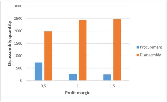
Impact of sale cost
To compute to identify the right business model, we fix 𝛽 to 1.8 and we vary the profit margin 𝛾 . As shown in Table 5, total and sale costs sharply increase when the profit margin becomes larger.
Table 5: Impact of sale cost on the total cost and cost items
𝛾 Total cost Sale cost Procurement cost Holding cost Backlogging cost Setup cost Overload cost 0.5 528530.875 589823 23339 6346 7532 20500 3575 1 1127389.000 1187951 8395 5496 6994 24500 15175 1.5 1718149.375 1782815 7327 2566 7296 31000 16475
Fig 5 describes the distribution of the quantities resulting from the disassembly and external purchase to satisfy the external demands over the planning horizon under different profit margin. When profit margin is relatively large, the optimal solution tends to disassemble so that it can increase the sale cost. This implies that the proposed model finds the optimal solution while considering the trade-offs between the relevant costs.
0 500 1000 1500 2000 2500 3000 0,001 0,01 0,1 1 10 100 1000 Di sa ss embly q u an ti ty Ratio Procurement Disassembly
Fig 5: Disassembly quantity under different sale cost
5.2 Performance tests
To show the performance of the proposed mixed integer linear programming model more generally, a number of randomly generated test problems are solved and the test results are reported in this section. The performance measures used are:
The numbers of optimal solutions obtained by CPLEX,
The percentage deviations from optimal solution (Note that the percentage deviations can be obtained directly from CPLEX),
The computation times in seconds required to obtain optimal solutions, CPU(s)
The computational tests were done on 750 randomly generated instances consist of 50 problems for each combination of five levels of the number of items (10, 20, 30, 40 and 50) and three levels of the number of the periods (10, 20, and 30). For each level of the number of items, 10 disassembly product structures (and hence totally 50 structures) were randomly generated. In the disassembly structures, the number of child items for each parent and its yield were generated from 𝐷~𝑈 (3, 6) and 𝐷~𝑈 (1, 3), respectively. Here, 𝐷~𝑈 (𝑎, 𝑏) is the discrete uniform distribution with [a, b]. Disassembly lead times were set to 0 and 1 with probabilities 0.3 and 0.7 respectively. The different instances of parameters are generated in the same manner as Section 5.1.
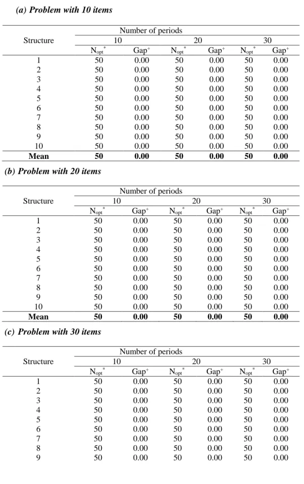
Table 7 summarizes the numbers of optimal solutions (obtained from CPLEX) and the percentage deviations from optimal solutions (or lower bound). As can be seen from the table 7, all the
0 500 1000 1500 2000 2500 3000 0,5 1 1,5 Di sa ss embly q u an ti ty Profit margin Procurement Disassembly
problems are solved optimally.The percentage deviations from the optimal solutions were within 0 per cent on average, which means that the CPLEX gives the optimal solution for all the product structure.
Table 7: Performance of the Mixed Integer linear Programming model
(a) Problem with 10 items
Number of periods
Structure 10 20 30
Nopt* Gap+ Nopt* Gap+ Nopt* Gap+
1 50 0.00 50 0.00 50 0.00 2 50 0.00 50 0.00 50 0.00 3 50 0.00 50 0.00 50 0.00 4 50 0.00 50 0.00 50 0.00 5 50 0.00 50 0.00 50 0.00 6 50 0.00 50 0.00 50 0.00 7 50 0.00 50 0.00 50 0.00 8 50 0.00 50 0.00 50 0.00 9 50 0.00 50 0.00 50 0.00 10 50 0.00 50 0.00 50 0.00 Mean 50 0.00 50 0.00 50 0.00
(b) Problem with 20 items
Number of periods
Structure 10 20 30
Nopt* Gap+ Nopt* Gap+ Nopt* Gap+
1 50 0.00 50 0.00 50 0.00 2 50 0.00 50 0.00 50 0.00 3 50 0.00 50 0.00 50 0.00 4 50 0.00 50 0.00 50 0.00 5 50 0.00 50 0.00 50 0.00 6 50 0.00 50 0.00 50 0.00 7 50 0.00 50 0.00 50 0.00 8 50 0.00 50 0.00 50 0.00 9 50 0.00 50 0.00 50 0.00 10 50 0.00 50 0.00 50 0.00 Mean 50 0.00 50 0.00 50 0.00
(c) Problem with 30 items
Number of periods
Structure 10 20 30
Nopt* Gap+ Nopt* Gap+ Nopt* Gap+
1 50 0.00 50 0.00 50 0.00 2 50 0.00 50 0.00 50 0.00 3 50 0.00 50 0.00 50 0.00 4 50 0.00 50 0.00 50 0.00 5 50 0.00 50 0.00 50 0.00 6 50 0.00 50 0.00 50 0.00 7 50 0.00 50 0.00 50 0.00 8 50 0.00 50 0.00 50 0.00 9 50 0.00 50 0.00 50 0.00
10 50 0.00 50 0.00 50 0.00
Mean 50 0.00 50 0.00 50 0.00
(d) Problem with 40 items
Number of periods
Structure 10 20 30
Nopt* Gap+ Nopt* Gap+ Nopt* Gap+
1 50 0.00 50 0.00 50 0.00 2 50 0.00 50 0.00 50 0.00 3 50 0.00 50 0.00 50 0.00 4 50 0.00 50 0.00 50 0.00 5 50 0.00 50 0.00 50 0.00 6 50 0.00 50 0.00 50 0.00 7 50 0.00 50 0.00 50 0.00 8 50 0.00 50 0.00 50 0.00 9 50 0.00 50 0.00 50 0.00 10 50 0.00 50 0.00 50 0.00 Mean 50 0.00 50 0.00 50 0.00
(e) Problem with 50 items
Number of periods
Structure 10 20 30
Nopt* Gap+ Nopt* Gap+ Nopt* Gap+
1 50 0.00 50 0.00 50 0.00 2 50 0.00 50 0.00 50 0.00 3 50 0.00 50 0.00 50 0.00 4 50 0.00 50 0.00 50 0.00 5 50 0.00 50 0.00 50 0.00 6 50 0.00 50 0.00 50 0.00 7 50 0.00 50 0.00 50 0.00 8 50 0.00 50 0.00 50 0.00 9 50 0.00 50 0.01 50 0.00 10 50 0.00 50 0.00 50 0.00 Mean 50 0.00 50 0.00 50 0.00
Nopt*: Number of problems (out of 50 problems) that solved optimally.
Gap+:Percentage deviation from the optimal solution (averaged over 50 problems for each product structure).
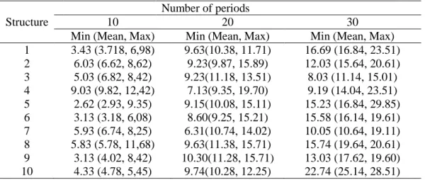
The test results summarized in Tables 8 represents the minimal, average and maximal values of the CPU(s) required by CPLEX. It can be seen from this table that the new mixed-integer linear programming model can gives the optimal solution for all the test problems within a reasonable amount of computation time. In fact, its CPU(s) do not exceed 42.16 in average. In summary, it can be concluded that the new MILP suggested in this paper can give the optimal solutions of the practical-sized problems within very short computation times. However, CPU time mainly depend on the problem data, such as disassembly structure, capacity time, cost values, etc.
Table 8: CPU seconds of the new mixed integer linear programming model
(a) Problem with 10 items
Number of periods
Structure 10 20 30
Min (Mean, Max) Min (Mean, Max) Min (Mean, Max) 1 0,125(0.324,0.547) 0.15(0.18,0.22) 0,24(0.47,1.15) 2 0,092(0.134,0.617) 0.09(0.15,0.51) 0,46(0.57,1.95) 3 0,152(0.724,0.923) 0.09(0.15,0.51) 0,11(0.47,0.55) 4 0,112(1.934,1.297) 0.19(0.20,0.43) 0,34(0.47,1.25) 5 0,089(0.564,0.946) 0,12(0.35,0.51) 0,13(1.07,2.12) 6 0,142(0.974,1.226) 0,29(0.31,0.40) 1,34(1.47,3.25) 7 0,092(0.589,0.932) 0,09(0.25,0.31) 0,29(0.77,3.59) 8 0,252(0.886,1.023) 0,19(0.88,0.92) 0,34(0.47,1.25) 9 0,122(0.798,0.973) 1,29(1.31,1.51) 1.04(1.07,2.95) 10 0,152(0.724,1.563) 0,09(0.24,0.50) 3,23(3.97,5.25) (b) Problem with 20 items
Number of periods
Structure 10 20 30
Min (Mean, Max) Min (Mean, Max) Min (Mean, Max) 1 0,35 (0.53, 1.15) 0,42 (0.61, 1.21) 9.68 (10.87, 16.15) 2 1,05 (1.93, 4.95) 3,02 (4.51, 8.91) 11.16 (13.18, 19.25) 3 1,56. (2.03, 3.95) 1.22 (2.90, 3.81) 10.86 (11.68, 15.25) 4 0,95 (1.63, 2.05) 1,92 (3.11, 6.91) 12.08 (15.75, 18.95) 5 0,22 (0.23, 0.45) 3.02 (3.51, 5.91) 9.16 (11.18, 19.25) 6 0,93 (1.53, 5.15) 2,92 (2.91, 6.16) 15. 76 (19.86, 29.56) 7 2,15 (2,93, 3.95) 0,92 (1.80, 5.98) 16.68 (18.28, 19.25) 8 0,85 (1,13, 2.05) 1,92 (2.01, 9.92) 10.38 (11.67, 16.37) 9 0,77 (0,93, 3.15) 0,42 (0.61, 1.21) 9.16 (11.98, 12.35) 10 1,05 (1,56, 3.92) 4.46 (5.01, 6.22) 9.06 (10.87, 14.56) (c) Problem with 30 items
Number of periods
Structure 10 20 30
Min (Mean, Max) Min (Mean, Max) Min (Mean, Max) 1 3.43 (3.718, 6,98) 9.63(10.38, 11.71) 16.69 (16.84, 23.51) 2 6.03 (6.62, 8,62) 9.23(9.87, 15.89) 12.03 (15.64, 20.61) 3 5.03 (6.82, 8,42) 9.23(11.18, 13.51) 8.03 (11.14, 15.01) 4 9.03 (9.82, 12,42) 7.13(9.35, 19.70) 9.19 (14.04, 23.51) 5 2.62 (2.93, 9.35) 9.15(10.08, 15.11) 15.23 (16.84, 29.85) 6 3.13 (3.18, 6,08) 8.60(9.25, 15.21) 15.58 (16.14, 19.61) 7 5.93 (6.74, 8,25) 6.31(10.74, 14.02) 10.05 (10.64, 19.11) 8 5.83 (5.78, 11,68) 9.63(11.38, 15.71) 15.74 (19.64, 20.61) 9 3.13 (4.02, 8,42) 10.30(11.28, 15.71) 13.03 (17.62, 19.60) 10 4.33 (4.78, 5,45) 9.74(10.28, 12.25) 22.74 (25.14, 28.51)
(d) Problem with 40 items
Number of periods
Structure 10 20 30
Min (Mean, Max) Min (Mean, Max) Min (Mean, Max) 1 9.65 (6.83, 9.92) 19.09 (19.88, 23.46) 21.06 (23.88, 25.34) 2 10.82 (11.33, 16.42) 12.65 (15.83, 19.92) 20.52 (25.52, 26.02) 3 8.02 (10.23, 15.22) 11.12 (12.88, 13.46) 27.89 (28.89, 29.04) 4 7.79 (9.19, 12.04) 15.01 (16.30,20.02) 12.60 (13.83, 25.92) 5 7.22 (8.48, 10.42) 10.52 (15.52, 16.02) 25.08 (25.68, 29.73) 6 10.01 (11.30, 15.02) 13.9 (16.35, 19.42) 19.01 (26.30,30.02) 7 8.03 (16.58, 19.20) 15. 95(18.85, 21.40) 24.05 (20.60, 26.74) 8 9.02 (9.33, 10.40) 19.9 (26.35, 29.42) 28.93 (30.58, 39.21) 9 13.9 (16.35, 19.42) 17.89 (19.09, 22.24) 29.73 (30.58, 39.21) 10 11.82 (12.33, 15.10) 18.45 (19.87, 20.40) 23.056 (23.608, 18. 34) (e) Problem with 50 items
Number of periods
Structure 10 20 30
Min (Mean, Max) Min (Mean, Max) Min (Mean, Max) 1 12,703 (12,99, 23,96) 15,84 (16,50, 18,40) 30,10 (32,53, 38,90) 2 10,89 (11,71, 22,21) 17,96 (18,87, 20,62) 27,24 (30, 36, 33,25) 3 15,18 (16,99, 18,96) 19,64 (19,90, 20,09) 31,12 (31,93, 32,25) 4 10,45 (13,45, 15,82) 18,36 (21,42, 24,68) 29,98 (31, 56, 32,35) 5 11,92 (12,72, 18,32) 16,41 (18,12, 20,35) 25,87 (29, 55, 35,12) 6 13,76 (20,33, 22,66) 25,94 (26,59, 28,25) 40,87 (42, 16, 59,25) 7 10,36 (11,65, 12,16) 23,15 (26,51, 28,56) 27,32 (28,63, 29,16) 8 15,19 (16,85, 18,34) 19,12 (20,48, 21,96) 36,28 (39, 26, 42,15) 9 20,37 (21,19, 22,68) 14,84 (16,50, 18,40) 30,93 (33,74, 36,36) 10 10,72 (13,96, 15,43) 23,74 (25,95, 28,46) 23,45 (30,68, 34,38) 6 Conclusion
In this research, we considered the capacitated disassembly planning problem in which we determine the timing and the optimal quantity of ordering the end-of-life products to fulfill the external demands of individual disassembled items over a given planning horizon. The objective is to maximize the profit while minimizing the sum of cost functions which one might encounter in practice, such as a setup cost for each non-leaf item, the sum of inventory holding, external procurement, disposal, backlogging costs for each non-root items and penalty cost for
overloading disassembly capacity along time horizon. A new mathematical formulation of R-MRP model was suggested. It is formulated as a mixed-integer linear programming (MIP) to represent and solve optimally the basic case of the problem, i.e. multi-period planning problem,
single product type and multi-level product structure. Sensitivity analyses on disassembly capacity, sale and procurement costs are also conducted, leading to the following useful insights: • Expanding the capacity maximize total cost. However, managers should carefully treat the trade-off between larger capacity investment, smaller costs and maximum of sales.
• The choice between buying and disassembling depends on economic considerations (procurement and sale costs).
The test results on a number of randomly generated problems showed that the new MIP model can give the optimal solution for all test problems within very short computation times. This research can be extended in several ways. First, it is interesting to consider the problem with parts commonality and multiple product types. Also, as in other disassembly problems, stochastic demands, disassembly lead times and yields are important subjects in disassembly planning problems.
References
Barba-Gutiérrez, Y., & Adenso-Díaz, B. (2009). Reverse MRP under uncertain and imprecise demand.
International Journal of Advanced Manufacturing Technology, 40(3–4), 413–424. doi:10.1007/s00170-007-1351-y
Barba-Gutiérrez, Y., Adenso-Díaz, B., & Gupta, S. M. (2008). Lot sizing in reverse MRP for scheduling disassembly. International Journal of Production Economics, 111(2), 741–751. doi:10.1016/j.ijpe.2007.03.017
Benaissa, M., Slama, I., & Dhiaf, M. M. (2018). Reverse Logistics Network Problem using simulated annealing with and without Priority-algorithm. Archives of Transport, 47(3), 7–17. doi:10.5604/01.3001.0012.6503
Gagnon, R. J., & Morgan, S. D. (2014). Remanufacturing scheduling systems : an exploratory analysis comparing academic research and industry practice, 4, 179–198.
Gao, N., & Chen, W. (2008). A genetic algorithm for disassembly scheduling with assembly product structure. Proceedings of 2008 IEEE International Conference on Service Operations and Logistics,
and Informatics, IEEE/SOLI 2008, 2, 2238–2243. doi:10.1109/SOLI.2008.4682907
Godichaud, M., Amodeo, L., & Hrouga, M. (2016). Metaheuristic based optimization for capacitated disassembly lot sizing problem with lost sales. Proceedings of 2015 International Conference on
Industrial Engineering and Systems Management, IEEE IESM 2015, (October), 1329–1335.
doi:10.1109/IESM.2015.7380324
Gupta, S. M., & Taleb, K. N. (1994). Scheduling disassembly. International Journal of Production
Research, 32(8), 1857–1866. doi:10.1080/00207549408957046
Gupta, S. M., Taleb, K. N., & Brennan, L. (1997). Disassembly of complex product structures with parts and materials commonality. Production Planning and Control, 8(3), 255–269. doi:10.1080/095372897235316
Hrouga, M., Godichaud, M., & Amodeo, L. (2016a). Heuristics for multi-product capacitated disassembly lot sizing with lost sales. IFAC-PapersOnLine, 49(12), 628–633. doi:10.1016/j.ifacol.2016.07.749 Hrouga, M., Godichaud, M., & Amodeo, L. (2016b). Efficient metaheuristic for multi-product
disassembly lot sizing problem with lost sales. IEEE International Conference on Industrial
Engineering and Engineering Management, 2016–Decem, 740–744. doi:10.1109/IEEM.2016.7797974
Inderfurth, K., & Langella, I. M. (2006). Heuristics for solving disassemble-to-order problems with stochastic yields. OR Spectrum, 28(1), 73–99. doi:10.1007/s00291-005-0007-2
Inderfurth, K., Vogelgesang, S., & Langella, I. M. (2015). How yield process misspecification affects the solution of disassemble-to-order problems. International Journal of Production Economics, 169, 56–67. doi:10.1016/j.ijpe.2015.07.016
Ji, X., Zhang, Z., Huang, S., & Li, L. (2016). Capacitated disassembly scheduling with parts commonality and start-up cost and its industrial application. International Journal of Production Research, 54(4), 1225–1243. doi:10.1080/00207543.2015.1058536
Kang, K. W., Doh, H. H., Park, J. H., & Lee, D. H. (2016). Disassembly leveling and lot sizing for multiple product types: a basic model and its extension. International Journal of Advanced Manufacturing
Technology, 82(9–12), 1463–1473. doi:10.1007/s00170-012-4570-9
Kim, D. H., Doh, H. H., & Lee, D. H. (2018). Multi-period disassembly levelling and lot-sizing for multiple product types with parts commonality. Proceedings of the Institution of Mechanical
Engineers, Part B: Journal of Engineering Manufacture, 232(5), 867–878. doi:10.1177/0954405416661001
Kim, D. H., & Lee, D. H. (2011). A heuristic for multi-period disassembly leveling and scheduling. 2011
IEEE/SICE International Symposium on System Integration, SII 2011, 762–767. doi:10.1109/SII.2011.6147544
Kim, H.-J., Lee, D.-H., & Xirouchakis, P. (2008). An Exact Algorithm for Two-Level Disassembly Scheduling TT - 2 수준 분해 일정계획 문제에 대한 최적 알고리듬. 대한산업공학회지, 34(4), 414–424. http://www.dbpia.co.kr/Article/NODE01914536
Kim, H. J., Lee, D. H., & Xirouchakis, P. (2006a). Two-phase heuristic for disassembly scheduling with multiple product types and parts commonality. International Journal of Production Research, 44(1), 195–212. doi:10.1080/00207540500244443
Kim, H. J., Lee, D. H., & Xirouchakis, P. (2006b). A Lagrangean heuristic algorithm for disassembly scheduling with capacity constraints. Journal of the Operational Research Society, 57(10), 1231– 1240. doi:10.1057/palgrave.jors.2602094
Kim, H. J., Lee, D. H., & Xirouchakis, P. (2007). Disassembly scheduling: Literature review and future research directions. International Journal of Production Research, 45(18–19), 4465–4484. doi:10.1080/00207540701440097
Kim, H. J., Lee, D. H., Xirouchakis, P., & Kwon, O. K. (2009). A branch and bound algorithm for disassembly scheduling with assembly product structure. Journal of the Operational Research
Society, 60(3), 419–430. doi:10.1057/palgrave.jors.2602568
Kim, H. J., Lee, D. H., Xirouchakis, P., & Züst, R. (2003). Disassembly scheduling with multiple product types. CIRP Annals - Manufacturing Technology, 52(1), 403–406. doi:10.1016/S0007-8506(07)60611-8
Kim, H. J., & Xirouchakis, P. (2010). Capacitated disassembly scheduling with random demand.
International Journal of Production Research, 48(23), 7177–7194. doi:10.1080/00207540903469035
Kim, J., Jeon, H., Kim, H., Lee, D., & Xirouchakis, P. (2005). Capacitated Disassembly Scheduling : Minimizing the Number of Products Disassembled, 538–547.
Kongar, E., & Gupta, S. M. (2002). A Multi-criteria Decision Making Approach for Disassembly-to-order Systems, 11(2), 171–183.
Kongar, E., & Gupta, S. M. (2006). Disassembly to order system under uncertainty. Omega, 34(6), 550– 561. doi:10.1016/j.omega.2005.01.006
Lambert, A., & Gupta, S. (2004). Disassembly Modeling for Assembly, Maintenance, Reuse and Recycling, 19. doi:10.1201/9780203487174
Langella, I. M. (2007). Heuristics for demand-driven disassembly planning. Computers and Operations
Research, 34(2), 552–577. doi:10.1016/j.cor.2005.03.013
Lee, D. H., Kim, H. J., Choi, G., & Xirouchakis, P. (2004). Disassembly scheduling: Integer programming models. Proceedings of the Institution of Mechanical Engineers, Part B: Journal of Engineering
Manufacture, 218(10), 1357–1372. doi:10.1243/0954405042323586
Lee, D. H., Rang, J. G., & Xirouchakis, P. (2001). Disassembly planning and scheduling: Review and further research. Proceedings of the Institution of Mechanical Engineers, Part B: Journal of
Engineering Manufacture, 215(5), 695–709. doi:10.1243/0954405011518629
Lee, D. H., & Xirouchakis, P. (2004). A two-stage heuristic for disassembly scheduling with assembly product structure. Journal of the Operational Research Society, 55(3), 287–297. doi:10.1057/palgrave.jors.2601690
Lee, D. H., Xirouchakis, P., & Zust, R. (2002). Disassembly scheduling with capacity constraints. CIRP
Annals - Manufacturing Technology, 51(1), 387–390. doi:10.1016/S0007-8506(07)61543-1
Liu, K., & Zhang, Z. H. (2018). Capacitated disassembly scheduling under stochastic yield and demand.
European Journal of Operational Research, 269(1), 244–257. doi:10.1016/j.ejor.2017.08.032
Morgan, S. D., & Gagnon, R. J. (2013). A systematic literature review of remanufacturing scheduling.
International Journal of Production Research, 51(16), 4853–4879. doi:10.1080/00207543.2013.774491
Neuendorf, K.-P., Lee, D.-H., Kiritsis, D., & Xirouchakis, P. (2001). Disassembly scheduling with parts commonality using Petri nets with timestamps. Fundamenta Informaticae, 47(3–4), 295–306. Prakash, P. K. S., Ceglarek, D., & Tiwari, M. K. (2012). Constraint-based simulated annealing (CBSA)
approach to solve the disassembly scheduling problem. International Journal of Advanced
Manufacturing Technology, 60(9–12), 1125–1137. doi:10.1007/s00170-011-3670-2
Taleb, K. N., & Gupta, S. M. (1997). Disassembly of multiple product structures. Computers & Industrial
Engineering, 32(4), 949–961. doi:10.1016/S0360-8352(97)00023-5
Tian, X., & Zhang, Z. H. (2018). Capacitated disassembly scheduling and pricing of returned products with price-dependent yield. Omega (United Kingdom). doi:10.1016/j.omega.2018.04.010
Ullerich, C., & Buscher, U. (2013). Flexible disassembly planning considering product conditions.
International Journal of Production Research, 51(20), 6209–6228. doi:10.1080/00207543.2013.825406
VoB, S., & Woodruff, D. L. (2003). Introduction to Computational Optimization Models for Production