The salesman and the tree: the importance of search in CP

HAL Id: hal-01436214

https://hal.archives-ouvertes.fr/hal-01436214

Submitted on 16 Jan 2017

HAL is a multi-disciplinary open access

archive for the deposit and dissemination of

sci-entific research documents, whether they are

pub-lished or not. The documents may come from

teaching and research institutions in France or

abroad, or from public or private research centers.

L’archive ouverte pluridisciplinaire HAL, est

destinée au dépôt et à la diffusion de documents

scientifiques de niveau recherche, publiés ou non,

émanant des établissements d’enseignement et de

recherche français ou étrangers, des laboratoires

publics ou privés.

The salesman and the tree: the importance of search in

CP

Jean-Guillaume Fages, Xavier Lorca, Louis-Martin Rousseau

To cite this version:

Jean-Guillaume Fages, Xavier Lorca, Louis-Martin Rousseau. The salesman and the tree: the

im-portance of search in CP. Constraints, Springer Verlag, 2016, 21, pp.145 - 162.

�10.1007/s10601-014-9178-2�. �hal-01436214�

The Salesman and the Tree:

the importance of search in CP

Jean-Guillaume Fages1_{, Xavier Lorca}1_{, and Louis-Martin Rousseau}2

1 _{TASC - Ecole des Mines de Nantes,}

{jean-guillaume.fages,xavier.lorca}@mines-nantes.fr

2

CIRRELT - Ecole Polytechnique de Montréal louis-martin.rousseau@cirrelt.net

Abstract. The traveling salesman problem (TSP) is a challenging opti-mization problem for CP and OR that has many industrial applications. Its generalization to the degree constrained minimum spanning tree prob-lem (DCMSTP) is being intensively studied by the OR community. In par-ticular, classical solution techniques for the TSP are being progressively generalized to the DCMSTP. Recent work on cost-based relaxations has improved CP models for the TSP. However, CP search strategies have not yet been widely investigated for these problems.

The contributions of this paper are twofold. We first introduce a natu-ral genenatu-ralization of the weighted cycle constraint (WCC) to the DCM-STP. We then provide an extensive empirical evaluation of various search strategies. In particular, we show that significant improvement can be achieved via our graph interpretation of the state-of-the-art Last Conflict heuristic.

1

Motivation

The traveling salesman problem (TSP) involves finding a Hamiltonian cycle of minimum weight in a given undirected graph G = (V, E) associated with a weight function w : E → Z. It has been widely investigated by the opera-tional research (OR) community for more than half a century, because it is an important optimization problem with many industrial applications. Its simple structure has enabled the development of general techniques, such as cutting planes, variable fixing, Lagrangian relaxation, and heuristics. These techniques are the key to the success of dedicated solvers (e.g., Concorde [3]), and they can be adapted to a range of optimization problems. Some have even been integrated into general MIP solvers, leading to great improvements in OR.

A natural extension of the TSP is the degree constrained minimum span-ning tree problem (DCMSTP). Given an undirected weighted graph G = (V, E) associated with a weight function w : E → Z and an integer array dmax, the

DCMSTP involves finding a minimum spanning tree (MST) of G for which every vertex v ∈ V has at most dmax[v]neighbors. In this way, a TSP can be

reduced to a DCMSTP in which for any v ∈ V , dmax[v] = 2. Consequently, the

From the constraint programming (CP) point of view, the TSP is very chal-lenging, because it is only slightly constrained, and the cost function is a major difficulty. This means that only a poor propagation can be expected from a ba-sic CP approach. However, when relaxations are considered, a good cost-based filtering can be achieved [7, 9]. Indeed, the most successful CP approaches to date owe their success to the introduction of relaxations, first introduced in OR, in the global constraints [2, 8]. From this perspective, the TSP allows us to study the behavior of CP solvers on problems that are dominated by optimization and to experiment with hybridization between CP and OR. However, search has not yet been widely investigated for this problem. Furthermore, none of the recent advances have been generalized to the DCMSTP, although such generalization is natural.

The contributions of this paper are twofold. First, in Section 2.2 we introduce a natural generalization of the weighted cycle constraint (WCC) [2] to the DCM-STP. Second, we empirically evaluate a wide range of graph search heuristics on the TSP and the DCMSTP. These heuristics are presented in Section 3. They include a graph adaptation of Last Conflict [15], which brings a greedy form of learning to the model. The experimental analysis (Sections 4 and 5) shows that significant improvement can be achieved by considering some simple graph properties at the search level. More precisely, the runtime is improved by up to four orders of magnitude over that of the state-of-the-art TSP approach of Benchimol et al. [2]. This pushes further the limits of CP, although dedicated OR solvers [3] remain ahead. For the DCMSTP, the results show that CP is a competitive approach.

2

The state-of-the-art CP models for the TSP and the DCMSTP

This section presents the state-of-the-art TSP model in CP (Section 2.2) and de-rives a DCMSTP model from it (Section 2.3). Since these models rely on a graph variable, we begin by providing an introduction to graph variables (Section 2.1).

2.1 Graph variables

Graph variables were introduced in [16]. We recall that a graph variable GRAPH has a domain defined by a graph interval dom(GRAPH) = [GRAPH, GRAPH]. A value for GRAPH is a graph included between GRAPH and GRAPH; see Figure 1 for an illustration.

The solving process involves adding to GRAPH (enforcing) some vertices and edges, and removing from GRAPH some other vertices and edges. Such operations are triggered by either filtering algorithms or the search process. These steps are performed until the graph variable is instantiated, i.e., until

GRAPH= GRAPH. In other words, GRAPH and GRAPH are respectively

A C D F G H (a) GRAPH A B C D E F G H (b) GRAPH A B C D E F G H (c) GRAPH compact domain representation A C D E F G H

(d) A possible value for GRAPH

Fig. 1.Graph variable illustration.

We use an undirected graph variable for which every vertex is mandatory, so the branching and filtering will concern only edges. More precisely, we use a binary search process in which each decision selects an unfixed edge, enforcing it in the left branch and removing it in the right branch. One can view the graph variable as an abstraction over a set of binary variables representing edges. In this representation, a decision selects a non-instantiated binary variable associ-ated with an edge, and tries to assign it first the value 1 and then 0. Additional information on graph variables can be found in [6, 17].

2.2 TSP state-of-the-art model

The state-of-the art CP formulation for the TSP uses a single graph variable GRAPHto represent the expected cycle and an integer variable Z to represent the objective function:

INPUT: Undirected graph G = (V, E)

Weight function w : E → Z

CP MODEL:

Minimize Z (1)

Constraint WCC(GRAPH, Z, w) (2)

Initial domains dom(GRAPH) = [(V, ∅), (V, E)], (3)

As can be seen, the TSP can be modeled as a minimization problem (1) involving a single graph constraint (2), the WCC, introduced by Benchimol et al. [2]. The graph variable GRAPH is defined (3) as a spanning subgraph of G. The domain of the objective variable Z (4) is initialized via the Lin–Kernighan– Helsgaun heuristic (LKH) [14], which is probably the most efficient heuristic for the TSP. No initial lower bound is given since the WCC propagation handles the lower bounding.

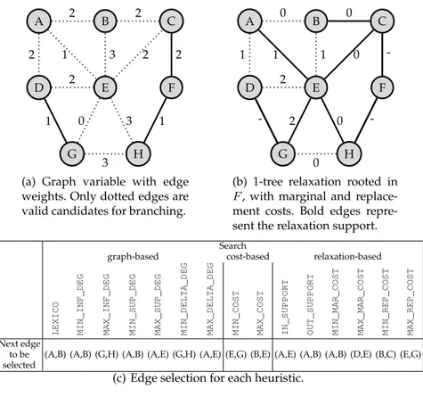
The WCC of Benchimol et al. [2] was a significant step forward that enabled CP to be competitive on instances of a reasonable size. This constraint is defined over a graph variable and embeds the 1-tree relaxation of Held and Karp [13], which provides a very powerful filtering. The 1-tree relaxation is roughly a care-ful adaptation of the minimum spanning tree relaxation to the case where a cy-cle is expected instead of a tree. More precisely, a 1-tree rooted in a vertex u ∈ V consists of a minimum tree spanning every vertex but u, plus the two cheap-est edges that are incident to u, so that the resulting relaxation has as many edges as a Hamiltonian cycle. This relaxation is improved with the subgradi-ent optimization of Held and Karp [13], which tends to the linear relaxation of the classical TSP linear programming model. In addition to lower bounding, back-propagation can be achieved from this relaxation: edges in (resp. out of) the relaxation support can be enforced (resp. removed) based on replacement (resp. marginal) costs [2]. The filtering rules of WCC are detailed in [2], and they mainly stem from [13, 18, 19], which form good further references. An illustra-tion is provided in Figure 2(c). This relaxaillustra-tion is rooted at vertex F and gives a lower bound of 12.

2.3 Extending the TSP model to solve the DCMSTP

From the above TSP model, we can naturally derive a CP model for the DCM-STP. It uses a single graph variable GRAPH to represent the expected tree, an array of n integer variables D to represent the vertex degrees, and an integer variable Z to represent the objective function:

INPUT: Undirected graph G = (V, E)

Weight function w : E → Z

Maximum degree function d : V → N

CP MODEL:

Minimize Z (5)

Constraint DCWSTC(GRAPH, Z, w, D) (6)

Initial domains dom(GRAPH) = [(V, ∅), (V, E)], (7)

dom(D[v]) = [1, d(v)], ∀v ∈ V (8)

dom(Z) = [−∞, +∞] (9)

The DCMSTP is modeled as a minimization problem (5) involving a single graph constraint (6), the degree constrained weighted spanning tree constraint (DCWSTC) that we introduce as a generalization of WCC. The graph variable GRAPHis defined as a spanning subgraph of G (7). The degree variables D are

defined according to the maximum degree function d (8). The domain of the objective variable Z has no initial bounds (9).

The DCWSTC is a direct generalization of the WCC in which the 1-tree is re-placed by a spanning tree, and the vertex degrees are no longer constrained to be 2 but are equal to the corresponding degree variable. It thus involves a La-grangian process that iteratively solves the MST problem and updates the cost function according to the violations of the degree constraints, as described in [1, 4]. The filtering rules are directly derived from the WCC.

In contrast to the TSP model, the DCMSTP model has no particular up-per bounding procedure. Since DCWSTC requires an upup-per bound for its sub-gradient method, we set up our own preprocessing step by simply changing the search strategy of the model. We compute a first solution by branching on the cheapest edges and propagating constraints (with Lagrangian relaxation turned off). Once a solution has been found, the solver restarts and the prepro-cessing is over. Thanks to the powerful DCWSTC filtering, the model is better at finding a good lower bound than improving the upper bound. Therefore, we use a bottom-up minimization strategy: instead of computing improving solu-tions, the solver aims to find a solution that has the value of the objective lower bound. If no such solution exists, then the objective lower bound is increased by one unit. This scheme is implemented by branching on the objective vari-able and enumerating its values. Once the objective varivari-able has been fixed, we must branch on the graph variable to either find a solution or prove that none exists. This paper focuses on the use of graph search heuristics for this step.

3

Studying graph search strategies

This section describes the application of various general heuristics to a graph variable. We also suggest several graph adaptations of Last Conflict [15], which may be useful for solving many other graph problems.

3.1 General graph heuristics

We believe that simpler heuristics are more likely to be used in different con-texts and therefore more likely to yield general results. We describe some heuris-tics that can naturally be applied to a graph variable, and we experimentally compare them in the next section:

– General graph heuristics consider only the graph variable: • LEXICO: Selects the first unfixed edge.

• MIN_INF_DEG (resp. MAX_INF_DEG): Selects an edge for which the sum of the endpoint degrees in GRAPH’s lower bound is minimal (resp. maximal).

• MIN_SUP_DEG (resp. MAX_SUP_DEG): Selects an edge for which the sum of the endpoint degrees in GRAPH’s upper bound is minimal (resp. maximal).

• MIN_DELTA_DEG (resp. MAX_DELTA_DEG): Selects an edge for which the sum of the endpoint degrees in GRAPH’s upper bound minus the sum of the endpoint degrees in GRAPH’s lower bound is minimal (resp. maximal).

– Weighted-graph heuristics have access to the cost function w:

• MIN_COST (resp. MAX_COST): Selects an edge with the minimal (resp. maximal) weight.

– Relaxation-based graph heuristics have access to a problem relaxation, pre-sumably embedded in a global constraint, which maintains a support, vari-able marginal costs, and varivari-able replacement costs:

• IN_SUPPORT (resp. OUT_SUPPORT): Selects an edge in (resp. out of) the support of the relaxation.

• MIN_MAR_COST (resp. MAX_MAR_COST): Selects an edge with the min-imal (resp. maxmin-imal) marginal cost, i.e., the edge outside the relaxation support for which enforcing involves the smallest (resp. largest) in-crease in the relaxation value.

• MIN_REP_COST (resp. MAX_REP_COST): Selects an edge for which the replacement cost is minimal (resp. maximal), i.e., the edge of the relax-ation support for which removal involves the smallest (resp. largest) increase in the relaxation value.

To keep this study simple, we break ties in a lexicographic manner. Figure 2 illustrates the behavior of the heuristics. Given the graph variable domain of Figure 2(a) and the relaxation of Figure 2(b), Figure 2(c) indicates the edge that each heuristic would branch on at the next decision.

It is worth mentioning that the TSP model of [2] uses MAX_REP_COST to branch on edges. However, it uses an opposite branching order: it first removes the selected edge and then enforces it upon backtracking. We found that the branching order had no significant influence on the results, so we decided to consider only the case where the edge is first enforced and then removed. This order is more natural, by analogy to integer variables for which decisions are usually value assignments, not value removals.

A B C D E F G H 2 2 2 1 3 2 2 3 1 2 1 0 3

(a) Graph variable with edge weights. Only dotted edges are valid candidates for branching.

A B C D E F G H 0 0 1 1 1 0 -0 -2 - 2 0

(b) 1-tree relaxation rooted in F, with marginal and replace-ment costs. Bold edges repre-sent the relaxation support.

Search

graph-based cost-based relaxation-based

LEXICO MIN_INF_DEG MAX_INF_DEG MIN_SUP_DEG MAX_SUP_DEG MIN_DELTA_DEG MAX_DELTA_DEG MIN_COST MAX_COST IN_SUPPORT OUT_SUPPORT MIN_MAR_COST MAX_MAR_COST MIN_REP_COST MAX_REP_COST Next edge

to be (A,B) (A,B) (G,H) (A,B) (A,E) (G,H) (A,E) (E,G) (B,E) (A,E) (A,B) (A,B) (D,E) (B,C) (E,G) selected

(c) Edge selection for each heuristic.

Fig. 2.Illustration of various strategies.

3.2 Adapting Last Conflict to graph problems

This paper focuses on exact approaches that are able to provide an optimality certificate. Because of the need to prove optimality, the search will presumably spend much time in infeasible regions of the search space. Hence, the Fail First principle [12] recommends first taking the decisions that are the most likely to fail, in order to get away from infeasible regions as soon as possible. To follow this principle, we apply a graph adaptation of the Last Conflict search pattern together with a heuristic.

Last Conflict [15] is a generic heuristic that is designed to be used together with any other heuristic, whence the term search pattern. We recall that its main rule is basically: If branching on some variable x yields a failure, then continue branch-ing on x. Let us consider a decision involvbranch-ing a variable x that resulted in a fail-ure. Last Conflict is based on the intuition that including x in the next decision would have a similar result, i.e., another failure. More precisely, there exists a minimal unsatisfiable set (MUS) of constraints [11], CMU S, that is responsible

for the failure that occurred. There is no guarantee that x is involved in a con-straint of CMU S. However, if x is not responsible for the unsatisfiability of the

problem, it has allowed propagation to determine that the problem was not sat-isfiable at the previous search node. This could be a matter of luck, or it could occur because the problem structure is such that x is strongly related to CMU S. If

so, and if the problem remains unsatisfiable after several backtracks, it is likely that branching on x will allow the solver to again determine the unsatisfiability. Thus, this process should speed up the recovery of a satisfiable state as well as the proof of optimality. For this reason, Last Conflict can be seen as a form of greedy learning, coming with no overhead.

In our case, the LKH heuristic [14] provides an extremely good initial upper bound for the TSP. Furthermore, since our DCMSTP model involves a bottom-up minimization, the objective bottom-upper bound of the DCMSTP is also low. Thus, both the TSP model and the DCMSTP model are presumably unsatisfiable dur-ing most of the search, and faildur-ing again is therefore desirable. However, when we use a single graph variable, Last Conflict is useless because any decision al-ready considers this variable. Thus, we must modify Last Conflict to achieve its expected behavior. We suggest a graph adaptation that involves a vertex, instead of a variable, in the last decision. The resulting branching rule is illus-trated in Figure 3. Whenever a decision over an edge (u, v) ∈ E is computed, one of its endpoints, say u, is arbitrarily chosen to be stored. While failure oc-curs, our graph interpretation of Last Conflict states that the next decision must involve an edge that is incident to u, if at least one such edge is unfixed. In other words, the heuristic continues branching in the same region of the graph, because it believes that there is more structure to exploit there.

We empirically investigate several policies for choosing the vertex to reuse after a failed branching decision over an edge (u, v) ∈ E:

– LC_FIRST: Reuses the first vertex, u.

– LC_RANDOM: Keeps both u and v in memory and randomly chooses which to reuse.

– LC_BEST: Keeps both u and v in memory and reuses that most suited for the heuristic. For instance, if MIN_COST is used, then this policy will select the vertex with the cheapest unfixed edge in its neighborhood.

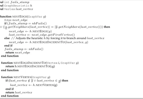
A simple way to implement LC_FIRST is given by Algorithm 1. This branch-ing rule adjusts the heuristic upon failure by restrictbranch-ing the decision scope to the subset of unfixed edges induced by the neighborhood of a given vertex (line 7), if this subset is not empty. Otherwise, while no failure occurs, the heuris-tic operates normally. For the sake of generality, we show how it can be used when branching on vertices as well (see theNEXTVERTEXfunction). However, in the context of the TSP, only edge selection is relevant because every vertex is mandatory.

Algorithm 1Implementation of LC_FIRST as a composite GraphHeuristic

global int f ails_stamp

global GraphHeuristic h global Vertex last_vertex

1:functionNEXTEDGE(GraphVar g)

2: Edgenext_edge

3: if (f ails_stamp = nbF ails()

∨ (|g.getN eighbors(last_vertex)| = |g.getN eighbors(last_vertex)|)) then

4: next_edge ← h.NEXTEDGE(g)

5: last_vertex ← next_edge.getF irstV ertex()

6: else// Adjusts the heuristic h by forcing it to branch around last_vertex

7: next_edge ← h.NEXTEDGEINCIDENTTO(last_vertex, g)

8: end if

9: f ails_stamp ← nbF ails()

10: return next_edge

11:end function 12:

13:functionNEXTEDGEINCIDENTTO(Vertex i, GraphVar g)

14: returnh.NEXTEDGEINCIDENTTO(i,g)

15:end function 16:

17:functionNEXTVERTEX(GraphVar g)

18: if(last_vertex /∈ g ∨ last_vertex ∈ g) then

19: last_vertex ← h.NEXTVERTEX(g)

20: end if

21: return last_vertex

22:end function

An illustration of the behavior of LC_FIRST with the MAX_COST heuristic is given in Figure 3. MAX_COST sequentially selects edges (B, E), (G, H), and (A, B). The constraint propagation then raises a failure, so the solver backtracks and removes edge (A, B). This leads to another failure, as well as the removal of edge (G, H), so the solver backtracks and deduces that edge (B, E) must be removed. Propagating this information leads to no failure, so a new decision has to be computed to continue the solving process. LC_FIRST now adjusts MAX_COSTby forcing it to use an edge around vertex A, because A was in the last decision. . . . (B, E) (G, H) (A, B) failure failure failure (A, ?) enforce remove

Fig. 3.Illustration of the search tree when using LC_FIRST with MAX_COST on the ex-ample. After a failure, the next decision must involve the last decision’s first vertex (A).

4

Experimental analysis for the TSP

4.1 Settings

Our implementation has been integrated into Choco-3.1.1, a Java library for constraint programming, so that the community can reproduce our results. The state-of-the-art model of [2] was implemented in C++; it was compiled with gcc with optimization flag -O3. All the experiments were performed on a Macbook

Prowith a 6-core Intel Xeon at 2.93 Ghz running MacOS 10.6.8 and Java

1.7. Each run had one core.

We considered the TSP instances of the TSPLIB data set, which is a refer-ence benchmark in OR. This library is a compilation of the most challenging TSP instances that have been studied in the literature. These instances are due to various authors and stem from routing, VLSI design, simulations, etc. We considered instances with up to 300 vertices, which seems to be the new limit for exact CP approaches on this benchmark.

This study is divided into two parts. First, we compare the heuristics of Section 3.1, together with the Last Conflict policies of Section 3.2 and the case where no policy is used, in order to highlight both good and bad design choices. Second, we compare the best model found with the state-of-the-art approach and measure the speedup we achieve.

4.2 Heuristic comparison

We now evaluate the heuristics suggested in Section 3.1, together with the graph-based Last Conflict policies of Section 3.2, to determine the best combination. To reduce the computational time, we consider the 42 simplest instances of the TSPLIB and use a time limit of one minute. Figure 4 gives the results for the various search heuristics, together with several Last Conflict policies. The policy NONEcorresponds to the case where we do not use any form of Last Conflict.

The best results are achieved by MAX_COST and MIN_DELTA_DEG. In con-trast, MIN_COST is surprisingly bad. This result confirms the intuition of the Fail-First principle on which our approach is based. Indeed, MIN_DELTA_DEG, which selects edges in sparse graph areas, may trigger failures from structure-based propagation, and MAX_COST, which selects expensive edges, may trigger failures from the 1-tree relaxation. This result also shows that simple heuristics perform better than more elaborate ones that require access to a problem relax-ation (to obtain marginal and replacement costs). Surprisingly, MAX_REP_COST does not give good results. Since it is used in the state-of-the-art model, this con-firms the claim that search plays an important role in the solution process and that it can still be improved.

Furthermore, whatever the policy, Last Conflict improves every search strat-egy evaluated. LC_FIRST allows us to solve 27% more instances on average. While it is the simplest policy, it performs better than both LC_RANDOM and

enables us to solve 41 of the 42 instances within the one-minute time limit. In-terestingly, the instance that remains unsolved varies from one heuristic to an-other. However, we were not able to solve all 42 instances by combining two heuristics. In summary, Last Conflict significantly improves the model, and im-portant performance differences can be observed from one heuristic to another.

(a) Graphical representation: whatever the search heuristic, it is always better to use it with one of the Last Conflict policies. LC_FIRSTand LC_BEST respectively provide the best results for 10 and 4 of the 15 tested heuristics.

Search

graph-based cost-based relaxation-based

Last

Conflict

policy

LEXICO MIN_INF_DEG MAX_INF_DEG MIN_SUP_DEG MAX_SUP_DEG MIN_DEL

T

A_DEG

MAX_DELTA_DEG MIN_COST MAX_COST IN_SUPPORT OUT_SUPPORT MIN_MAR_COST MAX_MAR_COST MIN_REP_COST MAX_REP_COST Minimum Average Maximum NONE 26 33 25 25 29 35 24 24 34 26 26 30 22 31 23 22 27.5 35 LC_FIRST 32 39 35 33 37 41 35 27 41 32 39 37 34 33 29 27 34.9 41 LC_BEST 31 38 30 35 38 39 28 27 40 30 36 41 31 36 27 27 33.8 41 LC_RANDOM32 38 34 31 37 40 33 27 40 29 36 37 30 33 26 26 33.5 40 Minimum 26 33 25 25 29 35 24 24 34 26 26 30 22 31 23 Average 30.3 37.0 31.0 31.0 35.3 38.8 30.0 26.3 38.8 29.3 34.3 36.3 29.3 33.3 26.3 Maximum 32 39 35 35 38 41 35 27 41 32 39 41 34 36 29

(b) Table representation, with minimum, average, and maximum: LC_FIRST, MIN_DELTA_DEG, and MAX_COST provide the best average results.

Fig. 4.Quantitative evaluation of search heuristics, together with various Last Conflict policies: number of instances among 42 simple instances of the TSPLIB solved within a one-minute time limit.

4.3 Pushing the limits of CP

We now compare our model to the state-of-the-art CP approach of Benchimol et al. [2], referred to as SOTA. For these comparisons we use MAX_COST with LC_FIRST, which appears to work well. We note that similar results are ob-tained when MIN_DELTA_DEG is used instead of MAX_COST.

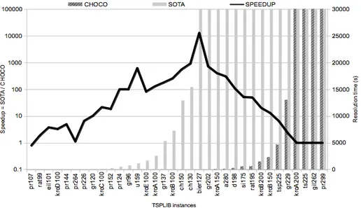
For this study, we increase the time limit to 30, 000 seconds to obtain a more precise evaluation of the speedup possible. We consider 34 challenging in-stances, with between 100 and 300 vertices, which represents the current limit of CP. The simpler instances are solved in less than a second by both approaches, whereas the harder ones cannot be solved by either approach. Figure 5 com-pares our approach with SOTA. The horizontal axis represents the instances. The first vertical axis shows the speedup (black), which is defined as the ra-tio of the solura-tion time of SOTA over the solura-tion time of CHOCO, with a log scale. The second vertical axis shows the solution time of CHOCO (dark gray) and SOTA (light gray), in seconds. The raw solution times are also provided.

Figure 5 shows that our heuristic gives a significant speedup on most in-stances. More precisely, the speedup is 511 on average, and it increases with the instance difficulty, up to four orders of magnitude (on bier127). The speedup then decreases because of the time limit. The solution time of the two approaches clearly shows that we have pushed the exponential further, from 100–200 to 200–300 vertices. This remains however below the performance of Concorde [3], the state-of-the-art TSP solver in OR (see [2] for a comparison).

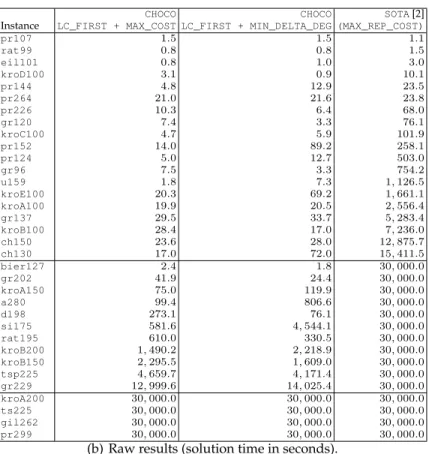
(a) Comparison of solution time in seconds for SOTA [2] and CHOCO with LC_FIRST and MAX_COST. The speedup is computed as the solution time of SOTA over the solution time of CHOCO. The speedup decrease is due to the time limit.

CHOCO CHOCO SOTA[2] Instance LC_FIRST + MAX_COST LC_FIRST + MIN_DELTA_DEG (MAX_REP_COST)

pr107 1.5 1.5 1.1 rat99 0.8 0.8 1.5 eil101 0.8 1.0 3.0 kroD100 3.1 0.9 10.1 pr144 4.8 12.9 23.5 pr264 21.0 21.6 23.8 pr226 10.3 6.4 68.0 gr120 7.4 3.3 76.1 kroC100 4.7 5.9 101.9 pr152 14.0 89.2 258.1 pr124 5.0 12.7 503.0 gr96 7.5 3.3 754.2 u159 1.8 7.3 1, 126.5 kroE100 20.3 69.2 1, 661.1 kroA100 19.9 20.5 2, 556.4 gr137 29.5 33.7 5, 283.4 kroB100 28.4 17.0 7, 236.0 ch150 23.6 28.0 12, 875.7 ch130 17.0 72.0 15, 411.5 bier127 2.4 1.8 30, 000.0 gr202 41.9 24.4 30, 000.0 kroA150 75.0 119.9 30, 000.0 a280 99.4 806.6 30, 000.0 d198 273.1 76.1 30, 000.0 si175 581.6 4, 544.1 30, 000.0 rat195 610.0 330.5 30, 000.0 kroB200 1, 490.2 2, 218.9 30, 000.0 kroB150 2, 295.5 1, 609.0 30, 000.0 tsp225 4, 659.7 4, 171.4 30, 000.0 gr229 12, 999.6 14, 025.4 30, 000.0 kroA200 30, 000.0 30, 000.0 30, 000.0 ts225 30, 000.0 30, 000.0 30, 000.0 gil262 30, 000.0 30, 000.0 30, 000.0 pr299 30, 000.0 30, 000.0 30, 000.0

(b) Raw results (solution time in seconds).

Fig. 5.Comparison with the state-of-the-art CP approach on challenging instances of the TSPLIB with a 30, 000-second time limit.

5

Experimental analysis for the DCMSTP

5.1 Settings

Our implementation has been integrated into Choco-3.1.0, a Java library for constraint programming, so that the community can reproduce our results. We reproduced the state-of-the-art approach of [5]. All our experiments were done on a Macbook Pro with a 6-core Intel Xeon at 2.93 Ghz running MacOS

10.6.8and Java 1.7. Each run had one core.

We consider the hardest DCMSTP instances in the literature, the data sets ANDINST, DE, and DR [4]. In the ANDINST and DE instances, each vertex is associated with a randomly generated point in the Euclidean plane. The cost function is then the Euclidean distance between the vertices. The maximum degree of each vertex is randomly chosen in [1, 4] for the ANDINST instances, and it is in [1, 3] for the DE instances. Thus, DE can be said to be harder to solve. In the set DR, the cost function associates with each edge a randomly

generated value in the range [1, 1000], and the maximum degree of each vertex is in [1, 3]. This last set is known to be hard to solve by existing approaches. The ANDINST instances have from 100 to 2, 000 vertices, while the DE and DR instances involve graphs of 100 to 600 vertices.

This study is divided into two parts. First, we compare the heuristics of Section 3.1, together with the Last Conflict policies of Section 3.2 and the case where no policy is used, in order to highlight both good and bad design choices. Second, we compare the best model found with the state-of-the-art approach and measure the speedup we achieve.

5.2 Heuristic comparison

We now extend the previous experimental analysis to the DCMSTP. As a first step, we evaluate the heuristics of Section 3.1, together with the graph-based Last Conflict policies of Section 3.2, to determine the best combination. To re-duce the computational time, we consider the 36 smallest instances and use a time limit of one minute. These 36 instances have up to 400 vertices, and they are evenly spread over the data sets ANDINST, DE, and DR. Figure 6 shows the number of instances that could be solved within the time limit, for each heuris-tic combination. NONE corresponds to the case where we do not use any form of Last Conflict.

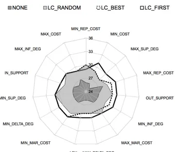
Fig. 6.Evaluation of search heuristics, together with various Last Conflict policies: num-ber of instances among the 36 smallest DCMSTP instances solved within a one-minute time limit. LC_FIRST provides the best results for every heuristic except one.

We make two observations. First, Last Conflict has a similar impact on the results as in the TSP case. Whatever the policy, it improves every search strategy evaluated. Furthermore, LC_FIRST again provides the best results on most of the problems. It gives a significant improvement, allowing us to solve 14% more instances on average.

Second, when LC_FIRST is used, all the search heuristics lead to similar results (between 29 and 31 solved instances). This is quite different from the observations for TSP instances.

5.3 Competitiveness of CP

We now compare our model to the state-of-the-art approach of Salles da Cunha and Lucena [5], referred to as SOTA. This method is inspired by techniques found in [3] that are used to solve the TSP. It combines local search, Lagrangian relaxation, filtering, and cutting planes. We used the MIN_SUP_DEG heuristic with LC_FIRST, which appears to work well for solving the DCMSTP with CP. For this study, because some of the instances are hard to solve, we increase the time limit to 30, 000 seconds. We consider all the instances of the data sets ANDINST, DE, and DR that were studied in [5]. Figure 7 depicts the improve-ment (or deterioration) over SOTA. The horizontal axis represents the instances. The first vertical axis shows the speedup (black), which is defined as the ratio of the solution time of SOTA to the solution time of CHOCO, with a log scale. The second vertical axis shows the solution time of CHOCO (dark gray) and SOTA (light gray) in seconds. Figure 7 is split according to the data sets.

Figure 7(a) shows that our CP approach to the DCMSTP is competitive with [5] on most easy Euclidean instances. However, it has difficulty solving three 2, 000-vertex instances. Since the input graphs are complete, this represents about two million edge instances. In the Euclidean case, when the maximum vertex degrees become more restricted (Figure 7(b)), the CP approach gets into trouble on smaller instances. More precisely, it cannot solve two instances, with 500and 600 vertices respectively, within the time limit. This indicates that, up to a certain size, CHOCO is competitive with SOTA. However, for large instances, the dedicated OR approach is more efficient. One reason that Euclidean in-stances are hard to solve in CP is the fact that the proximity relationship be-tween the vertices is transitive: if vertex A is close to vertex B and if B is close to C, then vertices A and C are also close. This impacts the behavior of the Lagrangian relaxation, which may have weak marginal costs and therefore an insufficient filtering. In contrast, CP is well suited to random instances (see Fig-ure 7(c)). CHOCO achieves a significant speedup over SOTA, up to two orders of magnitude. On such instances, the vertex proximity is no longer transitive, and so the propagation of any edge removal (or enforcing) through the DCWSTC provides a strong filtering. This enables CHOCO to solve every instance in less than three minutes, whereas SOTA takes, for example, more than two hours to solve dr_600_2.

(a) Easy Euclidean instances (ANDINST): CP and OR are comparable on most instances. CP has difficulty solving some 2, 000-vertex instances.

(b) Hard Euclidean instances (DE): CP has difficulty scaling over 400 vertices.

(c) Random instances (DR): CP beats OR!

Fig. 7.Comparison with the state-of-the-art OR approach for the DCMSTP (SOTA) [5], with a 30, 000-second time limit. The CHOCO model uses LC_FIRST and MIN_SUP_DEG. The speedup is computed as the solution time of SOTA over the solution time of CHOCO. The instances are sorted by increasing size.

6

Conclusion

This paper suggests a generalization of the WCC, which requires a graph vari-able to form a weighted spanning tree for which every vertex degree is con-strained. As the WCC requires an important implementation investment, this natural generalization is convenient.

We have presented an extensive experimental study of the ability of numer-ous general graph heuristics to solve the TSP and the DCMSTP. We decided to study simple and natural heuristics, which we believe are more likely to be implemented and extended to other problems than sophisticated and ded-icated ones are. Additionally, we have investigated several ways to adapt Last Conflict to graph variables. All of them improve the CP model, whatever the underlying heuristic. This gives a general significance to our results. Surpris-ingly, the experiments indicate that the simplest heuristics have the best per-formance, which is desirable. From a more practical point of view, we show how to improve the state-of-the-art CP approach for the TSP by up to four or-ders of magnitude, pushing further the limits of CP. We have shown that the CP model outperforms the state-of-the-art OR method on random DCMSTP in-stances. However, it does not yet compete with OR [3, 5] on the hardest TSP and DCMSTP instances.

Since Last Conflict is a greedy form of learning, a natural next step for the CP community would be to further investigate how learning can help the solution process, e.g., by explaining the WCC constraint. Recent work on explaining the circuitconstraint [10] provides a promising starting point.

References

1. Rafael Andrade, Abilio Lucena, and Nelson Maculan. Using Lagrangian dual infor-mation to generate degree constrained spanning trees. Discrete Applied Mathematics, 154(5):703–717, 2006.

2. Pascal Benchimol, Willem Jan van Hoeve, Jean-Charles Régin, Louis-Martin Rousseau, and Michel Rueher. Improved filtering for weighted circuit constraints. Constraints, 17(3):205–233, 2012.

3. Concorde TSP solver. http://www.tsp.gatech.edu/concorde.html.

4. Alexandre Salles da Cunha and Abilio Lucena. Lower and upper bounds for the degree-constrained minimum spanning tree problem. Networks, 50(1):55–66, 2007. 5. Alexandre Salles da Cunha and Abilio Lucena. A hybrid relax-and-cut/branch and

cut algorithm for the degree-constrained minimum spanning tree problem. Techni-cal report, Universidade Federal do Rio de Janeiro, 2008.

6. Grégoire Dooms, Yves Deville, and Pierre Dupont. CP(Graph): Introducing a graph computation domain in constraint programming. In Principles and Practice of Con-straint Programming, CP, volume 3709, pages 211–225, 2005.

7. Filippo Focacci, Andrea Lodi, and Michela Milano. Cost-based domain filtering. In CP, volume 1713 of Lecture Notes in Computer Science, pages 189–203. Springer, 1999. 8. Filippo Focacci, Andrea Lodi, and Michela Milano. Embedding relaxations in global constraints for solving TSP and TSPTW. Annals of Mathematics and Artificial Intelli-gence, 34(4):291–311, 2002.

9. Filippo Focacci, Andrea Lodi, and Michela Milano. Optimization-oriented global constraints. Constraints, 7(3–4):351–365, 2002.

10. Kathryn Glenn Francis and Peter J. Stuckey. Explaining circuit propagation. Con-straints, 19:1–29, 2013.

11. Maria J. García de la Banda, Peter J. Stuckey, and Jeremy Wazny. Finding all minimal unsatisfiable subsets. In PPDP, pages 32–43, 2003.

12. Robert M. Haralick and Gordon L. Elliott. Increasing tree search efficiency for con-straint satisfaction problems. In Proceedings of the 6th International Joint Conference on Artificial Intelligence - Volume 1, IJCAI’79, pages 356–364. Morgan Kaufmann Pub-lishers Inc., 1979.

13. Michael Held and Richard M. Karp. The traveling-salesman problem and minimum spanning trees: Part II. Mathematical Programming, 1:6–25, 1971.

14. Keld Helsgaun. An effective implementation of the Lin-Kernighan traveling sales-man heuristic. European Journal of Operational Research, 126(1):106–130, 2000. 15. Christophe Lecoutre, Lakhdar Sais, Sébastien Tabary, and Vincent Vidal.

Reason-ing from last conflict(s) in constraint programmReason-ing. Artif. Intell., 173(18):1592–1614, 2009.

16. Claude Le Pape, Laurent Perron, Jean-Charles Régin, and Paul Shaw. Robust and parallel solving of a network design problem. In Principles and Practice of Constraint Programming, CP, volume 2470, pages 633–648, 2002.

17. Jean-Charles Régin. Tutorial: Modeling problems in constraint programming. In Principles and Practice of Constraint Programming, CP, 2004.

18. Jean-Charles Régin. Simpler and incremental consistency checking and arc consis-tency filtering algorithms for the weighted spanning tree constraint. In Integration of AI and OR Techniques in Constraint Programming for Combinatorial Optimization Prob-lems, CPAIOR, volume 5015, pages 233–247, 2008.

19. Jean-Charles Régin, Louis-Martin Rousseau, Michel Rueher, and Willem Jan van Hoeve. The weighted spanning tree constraint revisited. In Integration of AI and OR Techniques in Constraint Programming for Combinatorial Optimization Problems, CPAIOR, volume 6140, pages 287–291, 2010.