1
A novel algorithm of cloud detection for water quality studies using 250 m downscaled 1
MODIS imagery 2
3
Claudie Ratté-Fortin*, Karem Chokmani, Anas El Alem 4
Institut National de la Recherche Scientifique, Centre Eau Terre Environnement, 490 De 5
la Couronne Street, G1K 9A9, Quebec city, Quebec, Canada. 6
7
*Corresponding author: [email protected] 8
Please cite this article as: Ratté-Fortin, C., Chokmani, K., and El-Alem, A. (2018). A 9
novel algorithm of cloud detection for water quality studies using 250 m downscaled 10
MODIS imagery. International Journal of Remote Sensing, 1-12. 11 12 13 14 15 16 17 18 19 20 21 22
Keywords: Cloud, mask, MODIS, chlorophyll-a, total suspended solids, dissolved 23
organic matter, inland waters, lakes, algal blooms, cyanobacteria. 24
2 Abstract
25
This study is part of a project aimed at developing an automated algorithm for algal 26
bloom detection and quantification in inland water bodies using Moderate resolution 27
imaging spectroradiometer (MODIS) imagery. An important step is to adequately detect 28
and exclude clouds and haze because their presence affects chlorophyll-a (chl-a) 29
estimations. Currently available cloud masking products appear to be ineffective in turbid 30
coastal waters. The purpose of this study is to develop a cloud masking algorithm based 31
on a probabilistic algorithm (Linear Discriminant Analysis) and designed for water 32
bodies by using MODIS images downscaled at a 250 m spatial resolution 33
(MODIS-D-250). Confusion matrix shows that the new cloud mask algorithm yields very 34
satisfactory results, enabling water classification for heavy turbid conditions with a mean 35
kappa coefficient ( (of 0.982 and a 95% confidence interval ranging from 0.979 to 36
0.986. The model also shows a very low commission error (sensitive to the presence of 37
haze) which is essential for accurate water quality monitoring, knowing that the presence 38
of clouds/haze/aerosols leads to major issues in the estimation of water quality 39
parameters. The cloud mask model applied on MODIS-D-250 images improves the 40
sensitivity to haze and the classification of turbid waters located at the edge of urban 41
areas better than the operational MODIS products, and it clearly shows an improvement 42
of the spatial resolution (250 m spatial resolution) compared to other cloud mask 43
algorithms (500 m or 1 km spatial resolution) leading to an increase in exploitable data 44
for water quality studies. 45
3 1. Introduction
47
Water colour satellite data are increasingly used to manage and monitor water quality for 48
ocean and coastal waters. In water colour data processing, good cloud masking is an 49
essential step in obtaining an accurate water colour signal. For that purpose, different 50
cloud mask algorithms have been developed but all have certain issues, specifically in the 51
processing of water colour data. In fact, a lot of these algorithms were developed 52
specifically for turbid water colour data, which leads to classification errors or to the loss 53
of valuable data (Chen & Zhang, 2015). Recently, efforts have been deployed to develop 54
explicit algorithms for cloud masking over turbid water colour data, but most were 55
applied on ocean and coastal waters (Wang & Shi, 2006; Banks & Mélin, 2015; Chen et 56
al., 2015). No cloud masking algorithm has been specifically designed for inland waters 57
(lakes, rivers, and estuaries), where water contains a lot more optically active components 58
such as chlorophyll-a (chl-a), total suspended solids (TSS), and coloured dissolved 59
organic matter (CDOM). 60
In ocean water studies, cloud detection techniques are generally based on the hypothesis 61
that the reflectance signal of water at near infrared (NIR) is almost null (Nagamani et al., 62
2015). This approach becomes, however, less effective with the presence of optically 63
active components in water, such as a high phytoplankton biomass, known to generate 64
turbid waters, which significantly increase reflectance at red and NIR channels (Kahru et 65
al., 2004). Turbid waters can be mistaken as cloud pixels, even under clear skies. 66
Moderate resolution imaging spectroradiometer (MODIS) Atmosphere Group developed 67
the standard MODIS cloud product generated at a 1 km and 250 m spatial resolution. 68
This product also uses a NIR threshold which is its principal weakness when applying the 69
4
algorithm on turbid waters (Robinson et al., 2003). Another 1 km-spatial resolution 70
algorithm developed by Nordkvist et al. (2009) and based on spectral variability of 71
visible and NIR often incorrectly mask intense phytoplankton blooms (Banks et al., 72
2015). Considering the high spatial variability of clouds, there are also algorithms based 73
on a spatial variability threshold of the MODIS green band (Martins et al., 2002) and the 74
MODIS NIR band (Nicolas et al., 2005). Once again, the use of visible and NIR bands 75
will identify turbid waters as clouds, due to their high spatial variability at these 76
wavelengths (Lubac & Loisel, 2007). To avoid this problem, certain cloud detection 77
algorithms use the MODIS shortwave infrared (SWIR) threshold such as that of Wang et 78
al. (2006) and Chen et al. (2015) who proposed a spatial variability threshold at SWIR 79
band. These cloud masks are generated at a spatial resolution of 1 km and 500 m 80
respectively. These methods based on SWIR band threshold appear to show the best 81
overall performance; however, they lack adequate spatial resolution for water studies in 82
small to medium-sized lakes. 83
This study is part of a project aimed at monitoring and assessing past, present and future 84
water quality in inland waters by using MODIS imagery downscaled to 250 m spatial 85
resolution (MODIS-D-250). In fact, the Canadian Center for Remote Sensing has 86
developed an approach allowing to downscale the spatial resolution of MODIS bands 3-7 87
from 500 m to 250 m (Trishchenko et al., 2006). Annexe products are also generated with 88
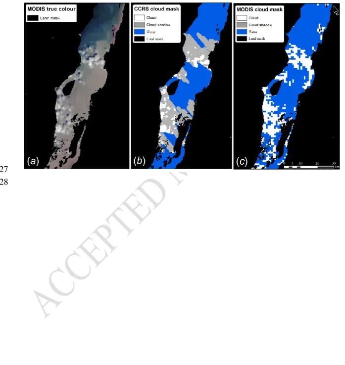
the downscaled images including a cloud mask at a spatial resolution of 250 m. However, 89
this model generally doesn’t perform well when detecting clouds and cloud shadows over 90
water bodies (see figure 1, centre). Furthermore, the actual cloud masking product 91
available for MODIS images is recorded at 250 m and 1 km spatial resolution (Ackerman 92
5
et al., 2010). The one generated at 1 km-spatial resolution is unsuitable for water quality 93
monitoring in small to medium-sized inland waters and in addition, it appears to be 94
ineffective in turbid coastal waters (see figure 1, right). The 250 m spatial resolution 95
MODIS cloud mask (Platnick et al., 2017) incorporates the results from the 1 km 96
resolution tests to maintain consistency with the 1-km cloud mask, and so, it appears to 97
show the same issues than the 1 km cloud mask in detecting thin clouds/haze and 98
distinguishing turbid waters. The Linear Discriminant Analysis (LDA) appears to be an 99
interesting alternative. This method, which is designed to highlight inland water bodies in 100
remotely sensed imagery, has often been used for land cover classification (Friedl & 101
Brodley, 1997; Xia et al., 2014; Priedītis et al., 2015) and for water index (Adrian Fisher 102
& Danaher, 2013). Indeed, multivariate techniques provide much richer and more global 103
information to the predictive model. The use of LDA is also preferred to threshold 104
algorithms when finding an optimal discriminant model. 105
The objective of this paper is to develop a cloud mask for water bodies (inland, coastal, 106
and open ocean) based on a LDA algorithm using MODIS-D-250 data. The present paper 107
focuses on the application of a probabilistic method using 1-7 MODIS-D-250 bands to 108
predict pixel classes, instead of actual parametric methods, as proposed in the literature 109
(threshold algorithms). 110
111
2. Material and Methods 112
2.1. Data collection and pre-processing 113
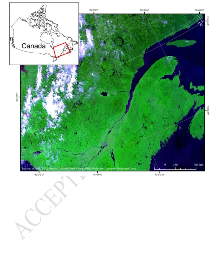
Satellite data that cover the southern part of the province of Quebec, Canada (44º-50º N, 114
67º-80º W) were acquired from MODIS sensor aboard the Terra platform of NASA’s 115
6
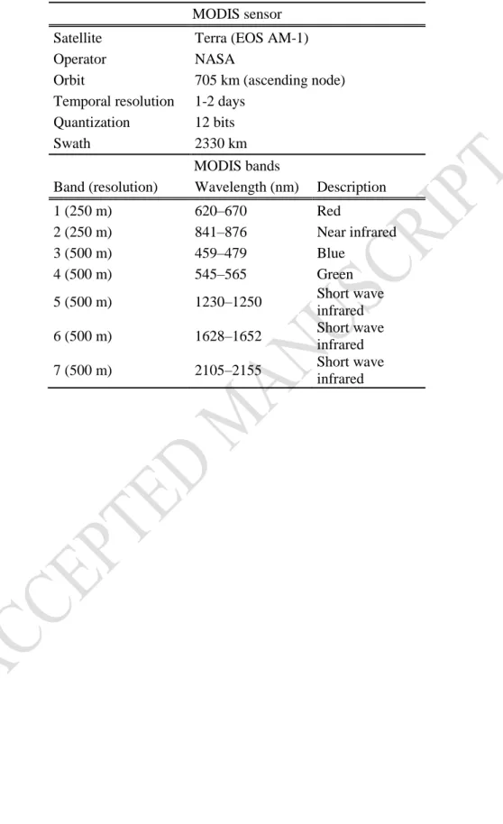
Earth Observation System (see figure 2). Characteristics of the MODIS bands used in this 116
study are presented in table 1. The spatial resolution of bands 3-7 was downscaled from 117
500 m to 250 m by using an adaptive regression and radiometric normalization as 118
described in Trishchenko et al. (2006). The approach used to downscale MODIS bands 3 119
to 7 from 500-m to 250 m spatial resolution (Trishchenko et al., 2006) was validated 120
using data at higher spatial resolution (Landsat ETM+ (30 m)). Results showed that the 121
downscaling procedure does not alter the radiometric properties of a scene, and so, the 122
higher resolution bands can be used to generate a reliable cloud mask at 250 m spatial 123
resolution. Besides, the MODIS bands originally at 250 m spatial resolution (bands 1-2) 124
and those downscaled (bands 3 to 7) are originally designed for aerosol, cloud and land 125
applications. Images were then re-projected from the Sinusoidal to the Lambert 126
Conformal Conic projection, and were corrected for atmospheric effects using the 127
Simplified Model for Atmospheric Correction (SMAC). Image pre-processing, including 128
downscaling, re-projection, and atmospheric correction was performed using an 129
automatic tool developed by the Canadian Center for Remote Sensing (Trishchenko et 130
al., 2007). Finally, in order to better distinguish water pixels from mixed pixels (land-131
water), a land mask developed by El Alem (2014) was applied to the MODIS database. 132
133
2.2. Model description 134
This section briefly describes the linear discriminant analysis modelling framework, 135
which was computed using Matlab software (R2016a). This method was proposed by 136
Ronald Fisher (1936) and consists of finding a projection that minimizes the variance 137
between classes while maximizing the distances between the projected means of the 138
7
classes. A general description of LDA can be found in Xanthopoulos et al. (2013). We 139
assume that we have a categorical dependent variable corresponding to the following 140
classes water, haze (a priori), and cloud, and independent variables corresponding to the 141
reflectance values of the 1-7 MODIS-D-250 bands. Independent variables are 142
transformed for normality. LDA allows to determine a subspace of dimension inferior to 143
that of the original data in which data are separable in terms of statistical measures of 144
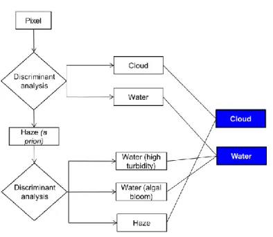
mean and variance values. First, the model discriminates the three classes (water, haze (a 145
priori), and cloud), assuming that independent variables have a multivariate normal 146
distribution and the same covariance matrix for each class (figure 3). Clear water is easy 147
to distinguish from cloud and fog due to the low reflectance in visible and near-infrared. 148
At the opposite, water containing optically active components such as TSS, CDOM and 149
chl-a is more difficult to distinguish from cloud/fog pixels in this spectral region. For that 150
reason, a second LDA is performed only on the pixels classified as fog to try to 151
discriminate real fog from waters with moderate to high chl-a concentrations or turbid 152
waters. The resulting data are further separated into three other classes: water (high 153
turbidity), water (algal bloom), and haze. A chl-a concentration estimator designed to 154
perform in optically complex inland waters (El-Alem et al., 2014) was used to manually 155
classify those three categories: fog, water (bloom), and water (turbidity). To classify 156
these categories, the chl-a concentration estimator was applied to images taken during 157
important algal blooms and on lakes known to have high turbidity. 158
159 160 161
8 2.3. Calibration and validation
162
A set of samples from twenty-six MODIS images were selected from the ice-free season 163
(May to November) of the years 2000 to 2015, and used for model calibration and 164
validation (table 2). We selected several free water samples (lakes, rivers, gulf, bay and 165
estuaries) from each MODIS scene that are representative of trophic classes of 166
waterbodies (oligotrophic, mesotrophic, eutrophic and hypereutrophic classes). Helped 167
by visual inspection of the maps and the highly turbid lakes known in the literature, a 168
chl-a concentration estimator designed to perform in optically complex inland waters (El-169
Alem et al., 2014) was also used to distinguish clear water, algal blooms and turbid 170
waters. The samples cover all the range of trophic classes based on very low chl-a 171
concentrations (0,1 g l–1) to very high chl-a concentrations (more than 1000 g l–1). 172
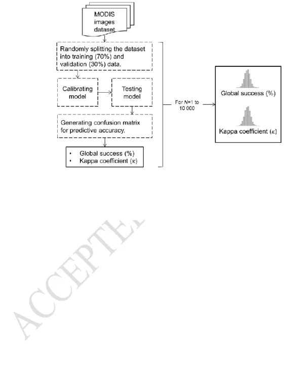
The dataset was then partitioned into two sets: we saved some images for calibration, 173
containing 70% (6186 pixels) of the data, and used the other for validation with 30% 174
(2651 pixels) of the data. The performance of the statistical model is evaluated using a 175
Monte-Carlo cross-validation: the random split of the original sample into calibration and 176
validation data is repeated 10,000 times in order to obtain a distribution of the global 177
success and the kappa coefficient ( values of the classification (see figure 4). To 178
evaluate the performance of the cloud mask algorithm, the model was applied to several 179
MODIS images (qualitative validation). These images were not used in the model 180
calibration/validation steps. Scenes that include lakes and estuaries known to be highly 181
turbid and lakes during a period when an algal bloom was occurring were selected. The 182
algorithm estimating chl-a concentration in inland waters (El-Alem et al., 2014) was also 183
applied to the validation images, allowing us to detect algal blooms. 184
9 3. Results and Discussion
185
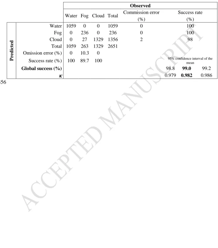
Table 3 presents the confusion matrix of the double discriminant analysis model over the 186
three classes. Results show that the classification of cloud and water pixels is not 187
problematic. The model adequately classifies water pixels with 0% false negative. The 188
model underestimates cloud detection in 1% of cases (false negatives) but those pixels 189
are classified as haze, which is not problematic for water colour data studies. 190
Consequently, none of the water pixels are misclassified as cloud or haze, which is the 191
major classification problem of actual cloud mask algorithms in presence of optically 192
active components (chl-a, TSS or CDOM) in water (Banks et al., 2015). Overall, the 193
model’s performance is very good with a of 0.982 and a 95% confidence interval 194
ranging from 0.979 to 0.986. Global success of the classification is 98.9% ranging from 195
99.0% to 99.2% (95% confidence interval). In order to compare our cloud mask 196
algorithm with the 250 m and 1 km MODIS cloud masks, we also have generated the 197
global success and over two classes (cloud, no cloud) into one combined cloud class. 198
Table 4 presents the results obtained with the three cloud masks applied on the same 199
validation data set. 200
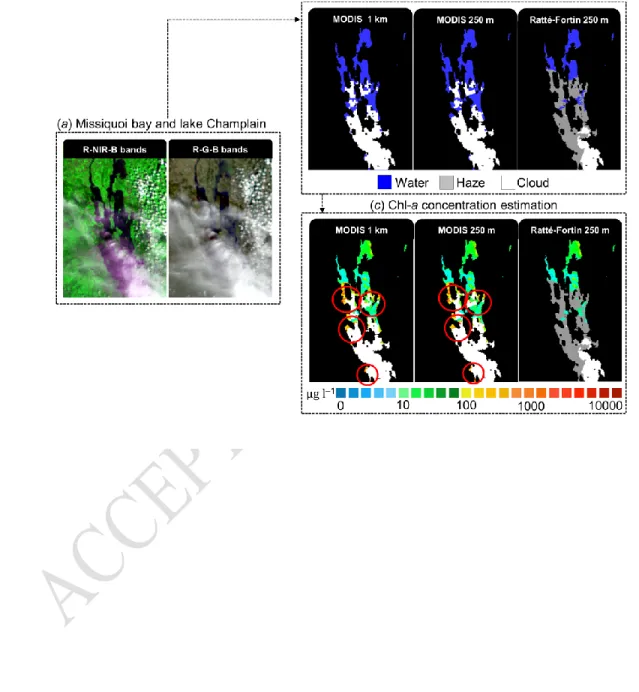
As a qualitative validation, the new cloud mask algorithm was applied to MODIS-D-250 201
images and compared to the current MODIS 1 km and 250 m cloud masks. Figures 5 and 202
6 present results for the Missisquoi Bay of Champlain Lake (during a period with 203
moderate to high chl-a concentration), St-Lawrence river (moderate turbidity and 204
moderate chl-a concentration) and Macamic Lake (high turbidity). MODIS cloud masks 205
don’t appear to be sensitive enough to haze, which leads to major issues in remote chl-a 206
estimates. Figure 5 shows an example of that issue and the improvement of haze 207
10
detection of our new algorithm. It presents the Missisquoi Bay during an algal bloom (at 208
the top) and the Champlain Lake covered in part with cloud and haze (at the bottom). The 209
three cloud masks are then presented (1km MODIS cloud mask, 250 m MODIS cloud 210
mask, and the new 250 m cloud mask), and below, the chl-a concentration estimated with 211
the remaining water pixels. The chl-a values were generated using an algorithm 212
developed by El-Alem et al. (2014). Both MODIS cloud masks are not enough sensitive 213
enough to haze, which yields some high estimates of chl-a concentration for pixels 214
without a priori algal bloom. 215
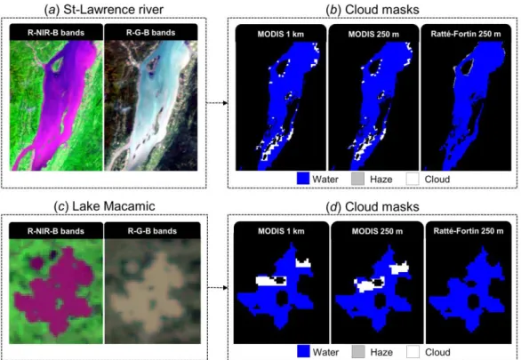
MODIS cloud masks are also not suited to perform well in turbid waters. It happens that 216
the masks falsely detect clouds in turbid waters. The St-Lawrence MODIS scene in figure 217
6 shows that the cloud/haze classification is highly improved with the new 250 m cloud 218
mask compared to both MODIS cloud masks. Highly turbid waters located at the edge of 219
an urban area, which are often problematic to cloud masking algorithms, are now much 220
better classified as water pixels. It should be noted that the land mask which was 221
developed and applied to the images covers transition zones from land to water (mixed 222
pixels) up to 250 m of the edge of lakes. Also, on small to medium-sized lakes and 223
particularly those with turbid waters, the false classification of MODIS cloud masks 224
becomes a major issue in terms of exploitable data. Figure 6 (bottom) shows another 225
MODIS scene on a smaller area, the Macamic Lake which has a surface area of 45 km2. 226
MODIS cloud masks falsely classify as cloud approximately 16 % of the lake area. 227
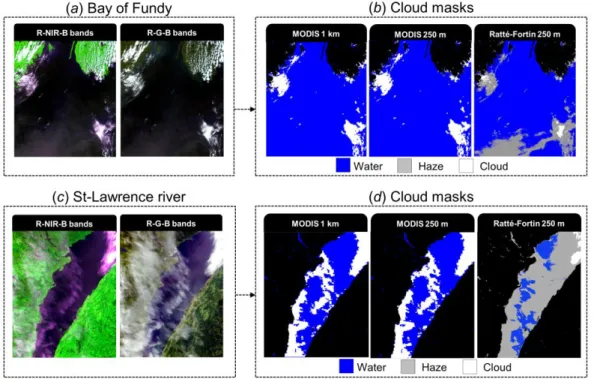
Figure 7 presents the cloud masks performance in thin haze and in cirrus conditions. The 228
image of the Bay of Fundy from 24 August 2014 shows the very good performance of the 229
algorithm in haze detection especially when compared to the MODIS cloud masks. The 230
11
second scene taken on St-Lawrence river clearly shows a lack of performance in 231
detecting cirrus clouds by the MODIS products. As we showed earlier, the lack of 232
sensitivity to haze and thin clouds can lead to misinterpretation of the water quality 233
parameters. 234
4. Conclusion 235
In conclusion, a cloud masking algorithm based on a double discriminant analysis at a 236
resolution of 250 m for MODIS imagery was presented. Overall, the new cloud mask 237
shows a better performance than the MODIS cloud mask when it is applied on turbid 238
waters, and particularly on highly turbid waters located at the edge of an urban area. The 239
new cloud mask presents an improved resolution of 250 m, leading to an increase of 240
exploitable data in the context of water colour studies, and particularly for water quality 241
monitoring in small to medium-sized inland waters. The new algorithm reduces potential 242
commission errors more efficiently than the MODIS cloud mask, which is less sensitive 243
to haze. The commission error reduction is essential for accurate algal blooms 244
monitoring, because the presence of clouds and haze affects chl-a concentration 245
estimations. Finally, the innovative aspect of this algorithm is the use of a probabilistic 246
method to generate a cloud mask compared to current methods proposed in the literature 247
based on threshold algorithms, leading to an optimal and accurate predictive model. 248
Confusion matrix results highlight the very good concordance between observed and 249
predicted classes using the algorithm on the downscaled MODIS bands, showing a global 250
success average of 99.6% with a 95% confidence interval ranging from 99.4% to 99.8%, 251
and a average of 0.993 with a 95% confidence interval ranging from 0.990 to 0.997. 252
12 References
253
Ackerman S, Strabala K, Menzel P, Frey R, Moeller C & Gumley L (2010) 254
Discriminating clear-sky from cloud with MODIS algorithm theoretical basis 255
document (MOD35. MODIS Cloud Mask Team, Cooperative Institute for 256
Meteorological Satellite Studies, University of Wisconsin. Citeseer. 257
Banks AC & Mélin F (2015) An assessment of cloud masking schemes for satellite ocean 258
colour data of marine optical extremes. International Journal of Remote Sensing 259
36(3):797-821. 260
Chen S & Zhang T (2015) An improved cloud masking algorithm for MODIS ocean 261
colour data processing. Remote Sensing Letters 6(3):218-227. 262
El-Alem A, Chokmani K, Laurion I & El-Adlouni SE (2014) An adaptive model to 263
monitor chlorophyll-a in inland waters in southern Quebec using downscaled 264
MODIS imagery. Remote Sensing 6(7):6446-6471. 265
El Alem A (2014) Développement d’une approche de suivi des fleurs d’eau d’algues à 266
l’aide de l’imagerie désagrégée du capteur MODIS, adaptée aux lacs du Québec 267
méridional. (Université du Québec, Institut national de la recherche scientifique). 268
Fisher A & Danaher T (2013) A water index for SPOT5 HRG satellite imagery, New 269
South Wales, Australia, determined by linear discriminant analysis. Remote 270
Sensing 5(11):5907-5925. 271
Fisher R (1936) The use of multiple measurements in taxonomic problems. Annals of 272
eugenics 7(2):179-188. 273
13
Friedl MA & Brodley CE (1997) Decision tree classification of land cover from remotely 274
sensed data. Remote sensing of environment 61(3):399-409. 275
Kahru M, Michell BG, Diaz A & Miura M (2004) MODIS detects a devastating algal 276
bloom in Paracas Bay, Peru. Eos, Transactions American Geophysical Union 277
85(45):465-472. 278
Lubac B & Loisel H (2007) Variability and classification of remote sensing reflectance 279
spectra in the eastern English Channel and southern North Sea. Remote Sensing of 280
Environment 110(1):45-58. 281
Martins JV, Tanré D, Remer L, Kaufman Y, Mattoo S & Levy R (2002) MODIS cloud 282
screening for remote sensing of aerosols over oceans using spatial variability. 283
Geophysical Research Letters 29(12). 284
Nagamani P, Latha TP, Rao K, Suresh T, Choudhury S, Dutt C & Dadhwal V (2015) 285
Setting of cloud albedo in the atmospheric correction procedure to generate the 286
ocean colour data products from OCM-2. Journal of the Indian Society of Remote 287
Sensing 43(2):439-444. 288
Nicolas J, Deschamps P, Loisel H & Moulin C (2005) Algorithm Theoretical Basis 289
Document, POLDER-2/Ocean Color/Atmospheric corrections.). 290
Nordkvist K, Loisel H & Gaurier LD (2009) Cloud masking of SeaWiFS images over 291
coastal waters using spectral variability. Opt. Express 17(15):12246-12258. 292
Platnick S, Meyer KG, King MD, Wind G, Amarasinghe N, Marchant B, Arnold GT, 293
Zhang Z, Hubanks PA & Holz RE (2017) The MODIS cloud optical and 294
14
microphysical products: Collection 6 updates and examples from Terra and Aqua. 295
IEEE Transactions on Geoscience and Remote Sensing 55(1):502-525. 296
Priedītis G, Smits I, Dagis S, Paura L, Krumins J & Dubrovskis D (2015) Assessment of 297
hyperspectral data analysis methods to classify tree species. Research for Rural 298
Development. International Scientific Conference Proceedings (Latvia). Latvia 299
University of Agriculture. 300
Robinson W, Franz B, Patt F, Bailey S & Werdell P (2003) Masks and flags updates. 301
Algorithm updates for the fourth Sea-WiFS data reprocessing, NASA Technical 302
Memorandum 206892:34-40. 303
Trishchenko A, Luo Y & Khlopenkov K (2006) A method for downscaling MODIS land 304
channels to 250 m spatial resolution using adaptive regression and normalization. 305
Remote Sensing for Environmental Monitoring 6366:36607-36607. 306
Trishchenko A, Luo Y, Khlopenkov K & Park W (2007) Multi-‐ spectral clear-‐ sky 307
composites of MODIS/Terra Land Channels(B1-‐ B7) over Canada at 250m 308
spatial resolution and 10-‐ day intervals since March, 2000: Top of the 309
Atmosphere (TOA) data. Enhancing Resilience in a Changing Climate. Earth 310
Sciences Sector Canada Centre for Remote Sensing (CCRS). Natural Resources 311
Canada. 312
Wang M & Shi W (2006) Cloud masking for ocean color data processing in the coastal 313
regions. IEEE Transactions on Geoscience and Remote Sensing 44(11):3196-314
3105. 315
15
Xanthopoulos P, Pardalos PM & Trafalis TB (2013) Linear discriminant analysis. Robust 316
Data Mining, Springer. p 27-33. 317
Xia J, Du P, He X & Chanussot J (2014) Hyperspectral remote sensing image 318
classification based on rotation forest. IEEE Geoscience and Remote Sensing 319
Letters 11(1):239-243. 320
321 322
16 Tables and Figures
323
Figure 1: (a) MODIS true color image, (b) corresponding cloud mask developed by the 324
Canadian Center for Remote Sensing and (c) cloud mask developed by MODIS 325
Atmosphere Group. 326
327 328
17
Figure 2: Geographic location of MODIS imagery historical database. 329
330 331
18
Figure 3: Detailed method used to distinguish between cloud and water classes using 332
discriminant analysis. 333
19
Figure 4: Details of the method used to estimate the distribution of the global success of 335
the classification (%) and using Monte-Carlo cross-validation. 336
20
Figure 5 : (a) MODIS R-NIR-B color and R-G-B color of the Missisquoi Bay and the 338
Champlain Lake, (b) the three cloud masks generated and (c) the corresponding chl-a 339
concentration layers estimated with the remaining water pixels left (bottom-right). The 340
red circles show high chl-a concentration values where there is a priori no bloom. 341
21
Figure 6 : MODIS R-NIR-B color and R-G-B color of the St-Lawrence river (a) and the 343
lake Macamic (c), and the corresponding three cloud masks (b) and (d). 344
22
Figure 7 : MODIS R-NIR-B color and R-G-B color of the Bay of Fundy (a) and the St-346
Lawrence river (c), and the corresponding three cloud masks (b) and (d). 347
23
Table 1: Characteristics of the MODIS bands used in this study. 349
MODIS sensor
Satellite Terra (EOS AM-1)
Operator NASA
Orbit 705 km (ascending node)
Temporal resolution 1-2 days
Quantization 12 bits
Swath 2330 km
MODIS bands
Band (resolution) Wavelength (nm) Description
1 (250 m) 620–670 Red 2 (250 m) 841–876 Near infrared 3 (500 m) 459–479 Blue 4 (500 m) 545–565 Green 5 (500 m) 1230–1250 Short wave infrared 6 (500 m) 1628–1652 Short wave infrared 7 (500 m) 2105–2155 Short wave infrared 350
24
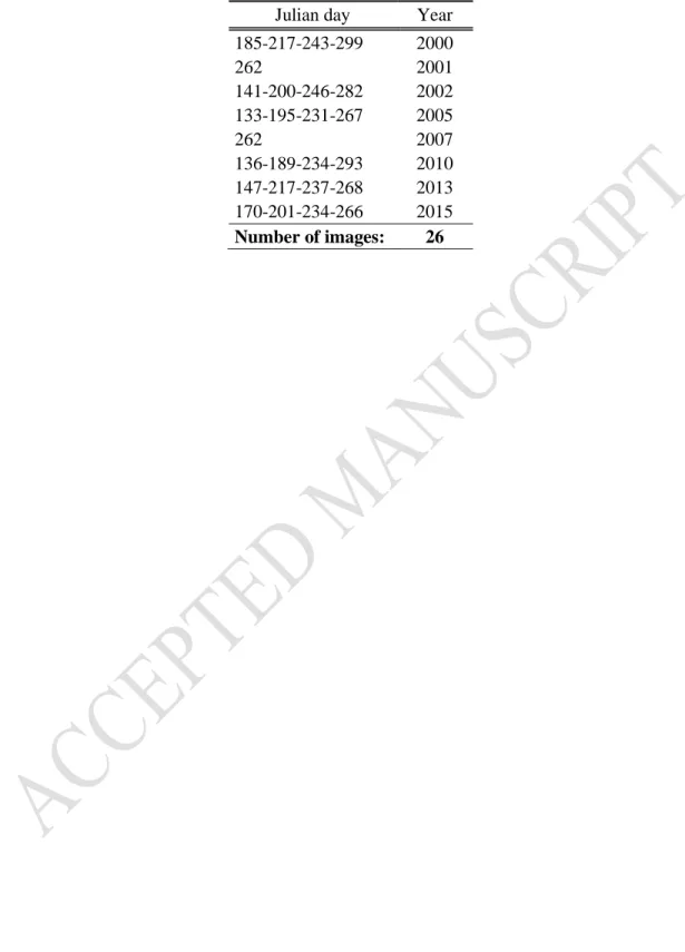
Table 2: List of the MODIS images used for the model calibration and validation. 351
Julian day Year
185-217-243-299 2000 262 2001 141-200-246-282 2002 133-195-231-267 2005 262 2007 136-189-234-293 2010 147-217-237-268 2013 170-201-234-266 2015 Number of images: 26 352
25
Table 3: Results of the double discriminant analysis confusion matrix with 95% 353
confidence intervals (percentile 2.5 and 97.5 of the distribution) of global success and 354
means. 355
Observed
Water Fog Cloud Total Commission error Success rate
(%) (%) Predi ct ed Water 1059 0 0 1059 0 100 Fog 0 236 0 236 0 100 Cloud 0 27 1329 1356 2 98 Total 1059 263 1329 2651 Omission error (%) 0 10.3 0
Success rate (%) 100 89.7 100 95% confidence interval of the mean
Global success (%) 98.8 99.0 99.2
0.979 0.982 0.986
26
Table 4 : Classification results of the two MODIS cloud products (1 km and 250 m) and 357
the proposed approach. 358
MODIS 1 km MODIS 250 m Ratte-Fortin
250 m
Global success (%) 91.3 95.3 99
0.827 0.905 0.982