W
HATM
OBILET
ERMINATIONR
EGIME FORA
SYMMETRICF
IRMS WITH AC
ALLINGC
LUBE
FFECT?
(Forthcoming in the International Journal of Management and Networks Economics)
Available at SSRN: http://ssrn.com/abstract=1088290
Patrice Geoffron1 Haobo Wang2
Summary: The aim of our paper is to determine the efficiency of asymmetric regulation of mobile termination rates (MTRs) in a market where firms are differentiated in size and with commercial offers including calling club effects. Major regulatory issues are related to these analyses, since some European National Regulatory Authorities and the European Commission tend to question asymmetric regulation mechanisms. Based on a model designed to determine firm profits and consumer surplus, our main results are the following: a) Asymmetric regulation of MTRs may contribute to increase welfare. If the impact is neutral regarding firms (simple reallocation of profits from the large to the small player), consumer surplus is increased; b) The appropriate way to proceed is to decrease the large firm’s MTRs, rather than increasing the smaller firm’s ones, which could produce negative side effects; c) From a dynamic point of view, appropriate asymmetric regulation may contribute to balance market shares and, in such a way, to compensate first mover advantages.
1 Introduction
As consumers are usually ignorant on Mobile Termination Rates (MTRs), collusion is a major concern in their setting. Starting from the works of Laffont, Rey & Tirole (1998 a, b) and Armstrong (1998), the general result obtained is that firm symmetry in market shares have incentives to increase their access charges in a logic of “double marginalization”. Furthermore, size symmetry may facilitate collusion, even without having recourse to access charges.
If these results are consistent for symmetric firms, one may wonder whether the reasoning should be modified when considering asymmetries. Indeed, asymmetric firms may have conflicting aims leading to more fragile collusive equilibriums. Thus, moving from “symmetry” to “asymmetry” to determine the effects of setting MTRs, and appropriate regulation, does not mean modifying a minor assumption. Recent works
1
) Corresponding author: Patrice Geoffron is Professor of Economics at the Université Paris-Dauphine, LEDa (Laboratory of Economics in Dauphine), Place du Maréchal de Tassigny, 75116, France, patrice.geoffron@dauphine.fr, +33660996733.
2
Haobo Wang is a telecommunications engineer, a graduate of the Ecole Nationale Supérieure des Telecommunications (Paris) and Tsinghua University (Beijing).
(Benzoni 2007, Dewenter 2007) highlight that European mobile markets are still impacted by first mover advantages, leading to long lasting asymmetries, taking such asymmetries into account is essential to determine appropriate regulation.
Regarding these issues, the conventional approach is that, in the early period of liberalization, asymmetric regulation (meaning differentiation of MTRs between mobile operators) is necessary to help entrants be competitive with the incumbent. Nonetheless, in the long run, when entrants are well established in the market, asymmetric regulation should be replaced by symmetric regulation of access charges at cost. This principle has been widely used by National Regulatory Authorities (NRAs) throughout Europe in the determination of MTRs to account for sequential market entry across all EU Member States. Nevertheless this differentiated treatment of mobile network operators’ MTR has been increasingly questioned by Member States. At the root of needs for a “sunset clause” on MTR asymmetry is the belief that initial disadvantages for the later entrants have either become negligible or are related to inefficient market entry, so that they may no longer be justified from a welfare point of view.
In the context of this regulatory debate, the aim of our paper is the following: to determine, with a model designed to consider asymmetric mobile operators proposing offers with a calling club effect, if asymmetric regulation of MTRs is consistent with an increase of consumer surplus and, in a dynamic perspective, efficient to balance market shares.
We will proceed as follows. After a literature review in section 2, our model will be presented in section 3. In section 4, we will carry out a simulation to highlight the main effect of asymmetric regulation on both welfare and market equilibrium. Research perspectives will be defined in conclusion.
2 Literature Review
Research on MTRs came to light in 1998, when both Laffont-Rey-Tirole (LRT from now on 1998 a, b) and Armstrong (1998) were published as milestone works. From then on, and up through the most recent working papers, two concerns have been always paid attention to: the collusive role of access charges and the advantage that larger or incumbent firms derived from this access charges framework. Miscellaneous factors have gradually been integrated into the research to fit with various market hypotheses. Regarding the risks of collusion, Armstrong (1998) indicated that for high access charges, symmetric operators use this tool to fuel their collusion in a linear tariff scenario that resembles the result of LRT (1998a). This point shows that equilibrium
between two firms can’t be reached when either access charges or substitutability are too high, whereas negotiated access prices can effectively lower this level of competition. Both Armstrong (1998) and LRT (1998a) evoke two part tariffs. With two part tariffs, however, access charges will not lower competition since it can lead to an increase in the cost per minute and not on the fixed price of a subscription. Operators can thus lower tariffs for fixed prices.
Another point regards inter-network and intra-network price discrimination and is put forward by LRT (1998b). They stress the network effects in the presence of such discrimination between two identical services, effects called “tariff mediated network externalities”. On a market where operators act symmetrically, this discrimination should be rewarded since welfare is increased.
For Carter and Wright (1999), the impact of brand loyalty is introduced to analyze unequal competition, but neither the on-net/off-net price discrimination nor club effects are accounted for. Given this framework, collusion by setting interconnection charges can be retained and non-reciprocal access charges can be used to set up market entry barriers. In their subsequent work, Carter and Wright (2003) assess an asymmetric market with brand loyalty. The authors state that incumbents with brand loyalty prefer cost-based access fees. Nevertheless, if brand loyalty is strong enough, all competitors have the same preference for cost-based access fees.
According to Gans and King (2001), both cost-based access charges and the bill-and-keep mode can be used to reduce competition. In a two part tariff structure, mobile network operators can benefit from a high subscription charge in spite of low (meaning, lower than marginal cost) access charges, since the latter reduces the appeal for new subscribers. Their points of view are opposed by Cambini and Valletti (2003) who tend to prove that the bill-and-keep mode can be beneficial to the social welfare due to positive impact of quality-focussed investments.
Call externality is another dimension in this literature family and is considered by Berger (2004, 2005) for linear and two-part tariff situations. The author concludes that, given linear tariffs on a symmetric market, competitors will still have the incentive to collude if access charges are set below cost and if on-net prices are below off-net prices. In the two-part tariff scenario, he demonstrates that the bill-and-keep mode can effectively raise welfare compared to the cost-based mode.
Dewenter (2005) focuses on the regulation of access charges in his work on markets presenting asymmetries in firm size. Based on the hypothesis that customers are ignorant about calling number termination, access charges tend to be higher since network externality is more evident, in accordance with Gans and King (2000). Dewenter also introduces asymmetry in competitor size as well as concomitant
regulation asymmetry. The results show that smaller operators can justify their increase in access charges since they have no significant influence on the wholesale price. Further, if larger operators are regulated unilaterally, the smaller operators may raise their access charge.
On these matters, Peitz (2005) insists on non-reciprocal regulation in an asymmetric market allowing entrants to charge a higher access fee compared to the incumbents. This framework will be socially desirable as it favours both new entrants and consumers’ surplus.
The emphasis of Hoernig (2007) lies in the differential between on-net and off-net tariff with the presence of receiving calls’ utility. Equilibrium in this context proves to be dependant on firms’ market share. Larger firms will consciously or not charge a higher off-net price, either under a linear or two-part tariff. The author also glimpses at the possibility of predatory pricing behaviour when that differential increases to a certain threshold.
In another recent paper, Gabrielsen & Vagstad (2007) explain how the calling club effect and switching costs influence a symmetric market. They show that within a symmetric market with reciprocal access charges, certain configurations of switching costs and access charges can lead to collusion instead of waging price wars against each other.
Our paper, on integrating certain practical market hypotheses, provides an overview on linear tariff competition between an incumbent and a later entrant. Call externality, mentioned in Berger’s two articles, is comprised in our modelling together with the calling club effect. Our goal is to discuss, within this given setting, the significance of regulating interconnection terminal charges and the possibility to re-establish the symmetry in the marketplace in accordance with the caution behind the “sunset clause”.
3 The Model
In our research, we set up our model on the base of LRT (1998 a,b) and Armstrong (1998). Other factors are also integrated to make the present model closer to certain real observed cases (persistent asymmetries in firms’ sizes and diffusion of offers with club effects).
• Consumer
Two differentiated network operators are located “à la Hotelling” at two ends of a unit line along which customers are uniformly distributed. In order to represent market asymmetries, we have adopted the method proposed in Behringer (2006) where subscribers derive different benefits from the selected network.
Firm 1, located at point 0, has a smaller user group compared to firm 2, located in the other end. Their market shares are noted separately as α1α2, and α1+α2 =1. Each
subscriber, whose location is different from 0 or 1, suffers from “undesirability” for not having the exact tailored service. Such undesirability is calculated by the distance from his location to that of the network multiplied by a transport cost t. This means that, if a customer at point x has subscribed to the service of network 2, his undesirability ist −1 x. Another way to express t is to use
t
2 1 =
σ which denotes substitutability between networks and, by the way, market competition.
Behringer (2006) used a differentiated utility amplifier factorη . Here we adapt his method by adding this factor β <1 exclusively for firm 2, incumbent as a first mover advantage. Thus, the undesirability of a customer at x suffers ∗x
σ
2 1
if he subscribes to firm 1 whereas if he subscribes to firm 2. This sufferance alters to 1−x
2σ β
withβ∈
( )
0,1 . Compared to Hoernig (2007) who added a priori disequilibrium σ β = A, we believe that this disequilibrium can better embody the network effect instead of a brand loyalty effect.Thus, in our “à la Hotelling” model, the market divides where the customer feels indifferent in choosing either side in terms of his welfare. Incumbent, firm 2, enjoys its advantage by less undesirability.
• Cost, price and utility
Each customer will incur a fixed cost fi for network i, and each call, despite the destination, adds a per-minute-cost c=c0 +c1+c0
c0 is the cost of originating and terminating a call whereas c is the cost of transmitting 1
access charge if one call happens to originate from network i and terminate on network j and network i pays j. Therefore a perceived cost of an off-net call can be represented as
0
c a c cioff = + j −
As the utility expression is concerned, we adopt the “traditional” way that began at LRT (1998 a,b) and other followers:
A customer can receive utility u(q) in making a call of q minutes,
( )
η η η η 1 1 − ∗ − = q q u (1)At the same time, when a customer is called, he also receives a certain utility that is proportioned to the caller’s. We note thereby u
( )
q =τ ∗u( )
q as the corresponding utility. η − = p p q )( (2) η− is therefore demand’s elasticity to price. u(q)can also be expressed by p:
η η η − ∗ − = 1 1 ) (p p u (3)
( )
p(
u( )
q pq)
v = maxq − (4) After FOC, the v(p) can be written as:η η − − = 1 1 1 ) (p p v (5)
Network operator i charges
(
Fi, pii, pij)
, the first is the fixed payment that supports the fixed cost of providing the service as well as the source of profit (to be proven further on). If we consider the linear tariff, then F=0.(
p ,ii pij)
is the retail price for on-net and off-net calls, otherwise the triplet combines to make the payment structure.Thus, the costs are classically divided into three parts: originating, transmitting and terminating, the last of which will be replaced by the MTR as a perceived cost. Quantity of consuming is a nonlinear function of price, and utility is also linked by consumed quantity.
• Calling club effect
Consumer behaviour breaks down into two categories as indicated by Gabrielsen and Vagstad (2007): “Tribe” calls and other calls which obey a balanced call pattern, i.e. the probability to call a subscriber is strictly equal. The significance of introducing a calling club comes from the observation in the European mobile market where more and more operators have already implemented a tribe numbers policy. The main idea is to offer a special price for one subscriber to call a certain fixed number of destinations, which might be his friends, his family or somebody with an important and steady demand for communication.
The prerequisite of such an offer is that all these subscribers belong to the same operators. The price is normally lower than other calls including on-net and calls are sometimes free, and thus labelled as unlimited. To facilitate modelling, we followed the assumption of Gabrielsen and Vagstad (2007) that pricing is fixed at the same level as on-net calls3. The proportion of tribe calls to total calls is a fixed parameter γ , which means that any subscriber has a probability of γ to call on the tribe and
(
1−γ)
to others among which on-net calls and off-net calls are determined by the ratio of market share of each network.• Market share in equilibrium
Until now, we can express the utility of a random customer situated at x and subscribing to network 1: x U σ ω 2 1 1 1 = − (6) Where: € ω1=γ1∗ v p
(
( )
11 + u q( )
11)
+ 1−(
γ1)
∗[
α1(
v p( )
11 + u q( )
11)
+α2(
v p( )
12 + u q( )
21)
]
− F1 (7)The utility of a customer at x and subscribing to network 2 is:
(
x)
U = − 1− 2 2 2 σ β ω (8) 3€
ω2=γ2∗ v p
(
(
22)
+ u q( )
22)
+ 1−(
γ2)
∗[
α2(
v p(
22)
+ u q( )
22)
+α1(
v p( )
21 + u q( )
12)
]
− F2 (9)The indifferent user in the Hotelling model is the point x whereU1
( )
x =U2( )
x , concretely, this point x is (also theα ): 1(
1 2)
1 2 1 β ω ω σ β β − + + + = x (10)In the symmetric situation (β =1), it is the same as traditional literature. Compared to Hoernig (2007), not only does the asymmetry parameter influence the basic cut (first item
β β +
1 ), utility is also amplified by1+β 2
. It is thus not difficult to solve the equilibrium market splitting point x is:
(
)
[
(
)
]
(
)
[
]
(
1 11 2 22 1 1 11 1 12 2 1 22 1 21 2 1)
1 ) 1 ( 1 1 1 1 2 1 F F h h h h h h − + − + − − − − + + − × + + + = α α γ α α γ γ γ β σ β β α (11)If we notehii =v
( ) ( )
pii +u qii ; hij =v( ) ( )
pij +u qji , then we solve α : 1(
)
(
)
(
)
[
]
(
)(
) (
)(
)
[
1 11 12 2 22 21]
1 2 22 2 12 1 22 2 11 1 1 1 1 2 1 1 1 1 2 1 h h h h F F h h h h − − + − − + − − + − − − + − + + + = γ γ β σ γ γ γ γ β σ β β α (12)To make the expression clearer:
(
)
(
)
(
)
[
1 11 2 22 1 12 2 22 2 1]
1 1 1 1 2 1 h h h h F F H − + − − − + − + + + = γ γ γ γ β σ β β (13)(
)
(
)
(
)
[
2 22 1 11 2 21 1 11 1 2]
2 1 1 1 2 1 1 F F h h h h H − + − − − + − + + + = γ γ γ γ β σ β (14) 2 1 H H H = + (15) Then, H H H H H 1 2 1 1 1 = + = α (16)(
)
H H H H H 2 2 1 2 1 2 1 = + = − = α α (17)• Profit and welfare
The profit of each firm comes from three parts: the fixed fee of subscription (this is optional in the linear tariff case); the revenue from calls part is the unforeseen part, since calls that fall in the network or the other together with the tribal part; with interconnection charges coming from the rival.
€
πi=αiγi
(
pii− c)
qii+αi(
1− γi)
[
αi(
pii− c)
qii+αj(
pij− c + a(
j− c0)
)
qij]
+αi(
Fi− fi)
+αiαj(
1− γj)
(
ai− c)
qji(18)
Under such circumstances, total consumer surplus for each network is separate (given certainα ):
( )
σ α ω α α 4 2 1 1 1 0 1 1 − =∫
U x dx (19)(
)
(
)
σ α β ω α α 4 1 1 ) ( 2 1 2 1 1 2 1 − − − =∫
U x dx (20)It is evident that the incumbent possesses a higher consumer surplus than the competitor even in a ceteris paribus situation (equal market share and utility providing ability). Total social welfare is:
€ W =π1+π2+ CS = α1γ1+α1 2 1−γ1
(
)
(
)
∗ 1+[
(
τ)
u q( )
11 − cq11]
+ α2γ2+α2 2 1−γ2(
)
(
)
∗ 1+[
(
τ)
u q( )
22 − cq22]
+α1α2{
(
1−γ1)
∗ 1+[
(
τ)
u q( )
12 − cq12]
+ 1−(
γ2)
∗ 1+[
(
τ)
u q( )
21 − cq21]
}
−α1f1−α2f2− α1 2 +βα2 2 4σFrom the social welfare point of view, the optimal price, if market is fixed, is:
τ + = 1 c pso (21)
4 Equilibrium with asymmetric tribe effect and linear tariff
In this part, we will study the equilibrium that emerges with different tariff schemes from two parts through a simulation. The rule of the game is that two firms separately set their own pricing package, including subscription fees, on-net price and off-net price. Customers then choose to subscribe to either firm (no right to abandon), resulting in subsequent market share, Profit will be calculated based on this data. We, therefore, assume that throughout this “game” the two firms are non-cooperative meaning the Cournot-Nash equilibrium will be established.
We will first determine how the market will be split if the incumbent possesses a larger tribe-effect and its rival a smaller one. Equilibrium prices, market shares, profit as well as total social welfare will be measured to assess the impact of each value of certain parameters. In the second part, we construct a dynamic process to test the effect and result of the regulatory “sunset clause”.
4.1 Comparison of the impact of two terminal-charge adjustment
measures
Market share in this discussion is set to be 25% versus 75%. Indeed, across the European mobile market, the market was dominated by one historical operator with another great challenger arriving a short time later, third and fourth (if exist) entrants always suffer from a “never-catching-up” syndrome4 explained by first mover advantages. Therefore defining such an allocation of market shares is a manner to characterize the basic division between the incumbents and later entrants.
Let’s assume that the tribe effect of the small firm is 10% compared with 30% of the larger one, this ratio being proportional to their market shares. To the regulators, the aim is to both foster long-term competition by favouring the later entrant and increase customer and social welfare. The only parameter that can be set outside the game is the MTR, which the regulator can change. We have, therefore, altered this parameter to observe the outcome.
The effort to counterbalance the innate discrepancy between two firms can be conducted in two ways, either raise the current access charge mark-up of the small firm (usually later entrant), or draw the terminal rate of incumbents down to the cost level.
4
Through simulation based on the model presented above, we have two tables of results (see Annex Table 7).
It is obvious that with such a favourable action, Firm1 will no doubt benefit from a larger market share as well as a higher profit. Firm2, i.e. the incumbent, loses in accordance market share and profit. It seems that disequilibrium is disappearing despite total welfare and consumer surplus is suffering a decrease thanks to this increase of the small firm’s MTR.
An alternative way to counterbalance the a priori disequilibrium between two firms is to lower the MTR’s incumbent towards cost level. Our simulation results are listed in Annex Table 8.
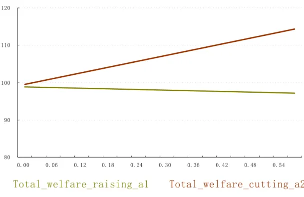
This table indicates a different scenario where market share and profit for the smaller firm shows a more effective increase (correspondingly, incumbent suffers more). What interests us is the increase of both total welfare and consumer surplus. We made a comparison in the Figures below to visualize this effectiveness.
80 90 100 110 120 0.00 0.06 0.12 0.18 0.24 0.30 0.36 0.42 0.48 0.54
Total_welfare_raising_a1
Total_welfare_cutting_a2
80 85 90 95 100 105 0.00 0.06 0.12 0.18 0.24 0.30 0.36 0.42 0.48 0.54
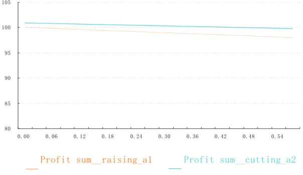
Profit sum__raising_a1 Profit sum__cutting_a2
Figure 2 : Sum of profit of two firms in two scenarios (trend line)
Figures 1 and 2 show the trend line of total welfare and profit sum as a result of adjustment. The trend line gives a clearer altering tendency compared with column Figures. All data is unified with respect to the original value which is transformed to 100 in the Figure’s vertical axis and the scale is zoomed within 80 to 120. As to the horizontal axis, the value is marked by the absolute increase or decrease of a1 or a2 for the convenience of comparison.
The two firms’ profit, which is the main part of total welfare, shows a quasi-constant level since terminal charges have a profit shift function versus increasing welfare.
80 90 100 110 120 130 140 150 0.00 0.06 0.12 0.18 0.24 0.30 0.36 0.42 0.48 0.54 profit1_by_raising_a1 profit1_by_cutting_a2 IsDO (profit1_by_cutting_a2) IsDO (profit1_by_raising_a1)
Figure 3: Comparison of entrant firm’s profit by increasing MTR1 and decreasing MTR2 Down to firm1, Figure 3 describes the profit increasing details. Obviously, lowering the incumbent’s MTR could provide an entrant with a much more effective increase in its profit compared to allowing it to raise its own MTR. Numerically, a 45%’s-plus increase is registered versus a slight drop in raising firm1’s terminal charges.
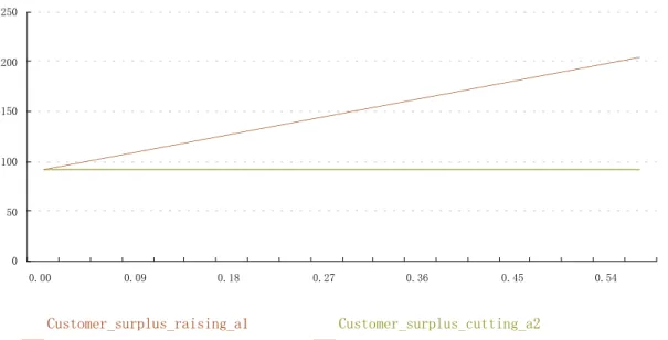
0 50 100 150 200 250 0.00 0.09 0.18 0.27 0.36 0.45 0.54 Customer_surplus_raising_a1 Customer_surplus_cutting_a2
IsDO (Customer_surplus_cutting_a2) IsDO (Customer_surplus_raising_a1)
Figure 4 finally indicates the great difference of benefit between the two measures. In terms of customer surplus, cutting MTR of incumbent may not only double the consumer’s surplus, but also force the incumbent to cut down its on-net price to keep its profit (see Table 7 and Table 8). Certainly, raising entrant’s MTR can have the same impact but the dimension is by far negligible.
4.2 Dynamic results
In this section, still using a dynamic simulation, we explore the possibility of resetting market symmetry with the prerequisite of rationality to pursue maximum profit of a later entrant’s firm.
One issue has been mentioned during the discussion dealing with asymmetric market in previous literature: the deadline of asymmetric regulation policy (if it is to be implemented for some time). The “sunset clause” advocates the presence of asymmetric policy, whereby the later entrant firm can actually practices two strategies targeting profit seeking (meaning rent seeking in fact) or at market share gaining.
Our model dynamically simulates the procedure that might take place when the regulator gradually shut down favorable asymmetric regulation policy. The entrant does not change its pursuit for profit, i.e. it sets its on-net and off-net price just to maximize its profit. Market share, however, is not particularly considered for the entrant.
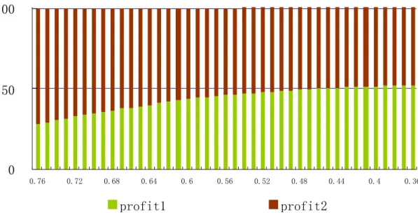
0.0% 50.0% 100.0%
0.76 0.72 0.68 0.64 0.6 0.56 0.52 0.48 0.44 0.4 0.36
marketshare1 marketshare2
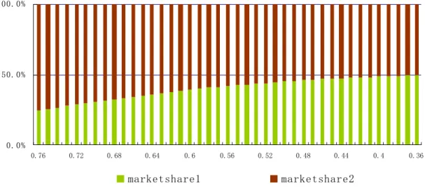
Figure 5 shows the impact on market share where the horizontal axis is the unit of period. At the beginning, the entrant’s terminal charge is set at a high level. Later on, as a result of the asymmetric regulation, the entrant’s market share and club effect increase. This new data will be brought into the next period as the basic set-up when the regulator slightly decreases the entrant’s terminal charge of the entrant.
The vertical axis of Figure 5 reflects the percentage change. Initial partitioning of the market is 1:3, and can also be considered as the ratio of calling club effect. Over time the two firms’ market share tends to converge, even though in a slower pace. In the last period, the terminal charges of both firms are equal and market share is 50% vs. 50%. With equal partitioning achieved before the whole de-asymmetry process, the regulator can thus stop whenever the market share of the later entrant has reached 50%.
0 50 100
0.76 0.72 0.68 0.64 0.6 0.56 0.52 0.48 0.44 0.4 0.36
profit1 profit2
Figure 6 : Impact of dynamic asymmetric regulation on profit
The entrant’s profit increases at almost the same speed as, if not higher than, its market share. It is worth noting that profit reached the 50% mark earlier than market share, due to higher access charge revenue. The gradual adjustment of asymmetric regulation on terminal charge works efficiently without much intervention in the frame of this model. In the meantime, our model shows that it is the length of time and frequency of adjustment that counts, as opposed to the total asymmetry quantity granted to the entrant.
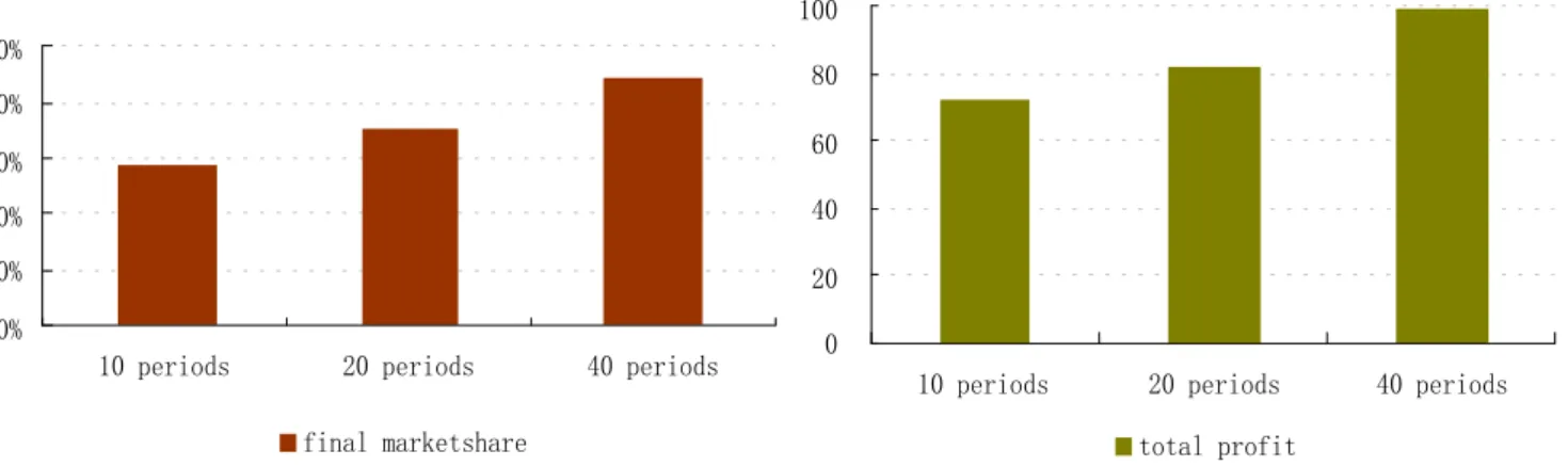
0% 10% 20% 30% 40% 50%
10 periods 20 periods 40 periods
final marketshare 0 20 40 60 80 100
10 periods 20 periods 40 periods total profit
Figure 7 : Comparing the different dynamics of de-asymmetry schemes
In Figure 7, we compare three possible de-asymmetry regulation schemes. In the model, regulators can divide a certain period into 10, 20 or 40 fragments with the initial and final value of the entrant’s terminal charge. Specifically, let’s suppose that the regulator authorizes the entrant to access mark-up as high as 40, for the case of 10 periods of asymmetry, the entrant will in period two to have a mark-up of 36, then 32 in period 3, until in the last period it has zero access mark-up, with each period including 4 time slots.
For up to 20-subdivisions, the entrant can have 40 as its access mark-up, then decrease 38, 36, 34 and until the last zero mark-up, each period lasts 2 time slots. This reasoning is the same as for the 40-subdivision case.
It is quite clear that the more frequent the change in asymmetric regulation policy (decrease of entrant’s access mark-up, to be specific) the more market share the entrant will seize by the end of asymmetric regulation. Total profits for entrant gains, follow the same law.
Therefore, we can draw the conclusion that for the dynamic simulation of de-asymmetry that when the regulator regularly alters the asymmetric policy on access mark-up for the entrant, the latter will automatically regain its market share to maximize its profit (by adjusting its on-net and off-net price). During this procedure, it is recommended that the regulator should reduce the entrant’s access mark-up and reduce it each time with a smaller part.
5 Conclusion
The aim of our paper was to determine the efficiency of asymmetric regulation of MTRs in a context where firms are differentiated in size and with commercial offers based on calling club effects. Major regulatory issues are related to these analyses, since some European National Regulatory Authorities and the European Commission tend to question asymmetric regulation due to the maturity of main national markets. But, since some of these markets may still be impacted by initial entry delays and various derived first mover advantages (brand loyalty, higher calling club effects, switching costs,…), our view is that the tools of asymmetric regulation should still be considered with attention and be kept in the scope of NRAs.
In the context of that debate, our main results are the following:
• Asymmetric regulation of MTRs may contribute to increase welfare. If the impact is neutral for the firms (simple reallocation of profits from the large to the small player), consumer surplus is augmented.
• The appropriate way to proceed is to decrease the larger firm’s MTRs, rather than increasing the smaller firm’s ones, that may lead to side effects which are contrary to the regulator’s aims.
• From a dynamic point of view, asymmetric regulation may contribute to balance market shares and, in such a way, erode the first mover advantages (meaning that the problem of the “sunset clause” would find a natural solution at the end of the game).
Of course, this process of balancing market shares would make no sense in a national context where market shares differences are the result of merits. But, since persistent first mover advantages (see Benzoni and Geoffron 2007) seems to still prevail in Europe, such regulation tools may not be neglected for the moment, especially given the current period of technological transition from 2G to 3G.
References
• Armstrong M. (1998), “Network Interconnection in Telecommunications” Economic Journal, Vol. 108, pp.545-564
• Benzoni L. (2007), “The “curse of the later entrants”: the case of the European mobile markets”, in Benzoni L. and Geoffron P. (eds.) (2007).
• Benzoni L. and Geoffron P. (eds.) (2007), Competition and Regulation with Asymmetries in Mobile Markets, Quanfitica Editions.
• Berger U. (2004), “Access charges in the presence of call externalities”,. Contributions to Economic Analysis & Policy 3(1), Article 21.
• Berger. U. (2005), "Bill-and-keep vs. cost-based access pricing revisited", Economics Letters 86 (1), 107-112.
• Berhinger S. (2006): “Asymmetric Equilibria and Non-Cooperative Access Pricing in Telecommunications”, mimeo, Universität Frankfurt.
• Cambini C. and Valletti T. (2003), "Network competition with price discrimination: bill-and-keep is not so bad after all", Economics Letters 81, 205–213.
• Carter, M. and Wright J. (1999), “Interconnection in network industries”, Review of Industrial Organization, 14, 1–25.
• Carter M. and Wright J. (2003), “Asymmetric network interconnection”, Review of Industrial Organization, 22, 27—46.
• Dewenter R. (2007), “First mover advantage in mobile telecommunications: the Swiss case”, in Benzoni L. and Geoffron P. (eds.) (2007).
• Dewenter R. and Haucap J. (2005), “The effects of regulating mobile termination rates for asymmetric networks”,. European Journal of Law and Economics 20, 185–197.
• Gabrielsen T.-S. and Vagstad S. ( 2007), “Why is on-net traffic cheaper than off-net traffic? Access markup as a collusive device and a barrier to entry”, European Economic Review, forthcoming.
• Gans J. and King S. (2001), “Using ‘bill and keep’ interconnect arrangements to soften network competition”, Economics Letters 71, 413–420.
• Hoernig S. (2007), “On-net and off-net pricing on asymmetric telecommunications networks”, Information Economics and Policy, 19, 2, 171-188.
• Laffont J.–J., Rey P. and Tirole, J. (1998a), “Network competition: I. Overview and non-discriminatory pricing”, The RAND Journal of Economics, 29, 1–37. • Laffont J.–J., Rey P. and Tirole J. (1998b), “Network competition: II. Price
discrimination”, The RAND Journal of Economics, 29, 38–56.
• Peitz M., (2005), “Asymmetric regulation of access and price discrimination in telecommunications”, Journal of Regulatory Economics, 28 (3), 327–343.
•
Annex
•
Parameters in the model and simulation
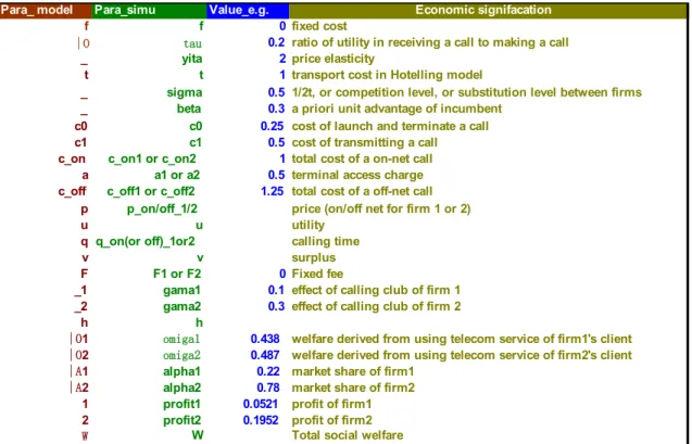
To make the model more comprehensive and clearer, we will list the parameters that correspond to modelling before and the code in the simulation.
Para_ model Para_simu Value_e.g.
f f 0 |O tau 0.2 _ yita 2 t t 1 _ sigma 0.5 _ beta 0.3 c0 c0 0.25 c1 c1 0.5
c_on c_on1 or c_on2 1
a a1 or a2 0.5
c_off c_off1 or c_off2 1.25
p p_on/off_1/2 u u q q_on(or off)_1or2 v v F F1 or F2 0 _1 gama1 0.1 _2 gama2 0.3 h h |O1 omiga1 0.438 |O2 omiga2 0.487 |A1 alpha1 0.22 |A2 alpha2 0.78 1 profit1 0.0521 2 profit2 0.1952
W W Total social welfare
Fixed fee
price (on/off net for firm 1 or 2) utility
calling time surplus
profit of firm1 profit of firm2 market share of firm1 market share of firm2 effect of calling club of firm 1
welfare derived from using telecom service of firm1's client effect of calling club of firm 2
welfare derived from using telecom service of firm2's client total cost of a off-net call
Economic signifacation
1/2t, or competition level, or substitution level between firms a priori unit advantage of incumbent
cost of launch and terminate a call total cost of a on-net call
terminal access charge cost of transmitting a call fixed cost
ratio of utility in receiving a call to making a call price elasticity
transport cost in Hotelling model
Table 1 : Parameters of model and simulation
•
Simulation results
Raw data that we derive from our simulation based on Matlab are presented in this section, including: isolated impact of calling club, impact of a priori advantage, impact of substitutability (competition level), impact of call externality (ratio of utility in receiving a call to originating a call) as well as the function of adjusting terminal charge.
P_on1 p_off1 p_on2 p_off2 marketshare1 marketshare2 profit1 profit2 Total_welfare Customer_surplus
gama +
-
+
=
-
+
-
+
-
+
+
beta +
=
+
=
=
+
-
+
-
-
-tau +
-
+
-
+
-
+
-
-
then+
+
+
sigma +
-
-
-
-
-
+
-
+
+
+
Table 2 : Impact of various parameters on indicators
When the tribe effect for a small firm increases, it has an interest to lower its on-net price and raise off-net prices for the intuitive reason that less off-net calls are needed and higher prices will result in a higher profit. Total social welfare and consumer surplus head up.
gama1 p_on1 p_off1 p_on2 p_off2 marketshare1 marketshare2 profit1 profit2 Total Welfare ConsumerSurplus
0.05 1.8 2.125 1.9 2.625 22.01% 77.99% 0.050 0.197 0.582 0.334 0.06 1.7 2.125 1.9 2.625 22.23% 77.77% 0.050 0.197 0.583 0.336 0.07 1.7 2.125 1.9 2.625 22.34% 77.66% 0.051 0.197 0.584 0.336 0.08 1.7 2.125 1.9 2.625 22.45% 77.55% 0.051 0.196 0.584 0.337 0.09 1.6 2.125 1.9 2.500 22.81% 77.19% 0.052 0.195 0.588 0.341 0.10 1.6 2.125 1.9 2.500 22.93% 77.07% 0.052 0.195 0.589 0.341 0.11 1.6 2.125 1.9 2.500 23.06% 76.94% 0.053 0.194 0.589 0.342 0.12 1.6 2.125 1.9 2.500 23.19% 76.81% 0.053 0.194 0.589 0.342 0.13 1.6 2.125 1.9 2.500 23.32% 76.68% 0.053 0.194 0.589 0.342 0.14 1.6 2.125 1.9 2.500 23.45% 76.55% 0.054 0.193 0.589 0.343 0.15 1.6 2.125 1.9 2.500 23.58% 76.42% 0.054 0.193 0.590 0.343 0.16 1.5 2.125 1.9 2.500 24.17% 75.83% 0.054 0.191 0.592 0.346 0.17 1.5 2.125 1.9 2.500 24.33% 75.68% 0.055 0.191 0.592 0.347 0.18 1.5 2.125 1.9 2.375 24.45% 75.55% 0.056 0.190 0.596 0.350 0.19 1.5 2.125 1.9 2.375 24.60% 75.40% 0.056 0.190 0.596 0.350 0.20 1.5 2.250 1.9 2.375 24.51% 75.49% 0.057 0.189 0.593 0.347 0.21 1.5 2.250 1.9 2.375 24.67% 75.33% 0.057 0.189 0.593 0.347 0.22 1.5 2.250 1.9 2.375 24.83% 75.17% 0.057 0.188 0.593 0.348 0.23 1.5 2.250 1.8 2.375 24.38% 75.62% 0.056 0.188 0.609 0.365 0.24 1.5 2.250 1.8 2.375 24.54% 75.46% 0.057 0.187 0.609 0.365
Table 3 : Impact of calling club effect
While gama1 is then set at 0.1 is in proportion to their market share ratio, we have the following tables for each parameter.
beta P_on1 p_off1 p_on2 p_off2 marketshare1 marketshare2 profit1 profit2 Total_welfare ConsumerSurplus
0.15 1.3 2.000 1.9 2.500 14.69% 85.31% 0.0307 0.2153 0.6485 0.4025 0.16 1.3 2.000 1.9 2.500 15.67% 84.33% 0.0327 0.2130 0.6448 0.3991 0.17 1.4 2.000 1.9 2.500 16.08% 83.92% 0.0347 0.2119 0.6403 0.3938 0.18 1.4 2.000 1.9 2.500 16.99% 83.01% 0.0366 0.2097 0.6367 0.3905 0.19 1.4 2.125 1.9 2.500 17.53% 82.47% 0.0385 0.2074 0.6303 0.3843 0.20 1.4 2.125 1.9 2.375 18.40% 81.61% 0.0409 0.2052 0.6294 0.3833 0.21 1.4 2.125 1.9 2.375 19.27% 80.73% 0.0428 0.2030 0.6261 0.3803 0.22 1.4 2.125 1.9 2.375 20.13% 79.88% 0.0447 0.2008 0.6229 0.3774 0.23 1.4 2.125 1.9 2.375 20.97% 79.03% 0.0466 0.1987 0.6198 0.3745 0.24 1.4 2.125 1.9 2.375 21.80% 78.20% 0.0484 0.1966 0.6168 0.3719 0.25 1.4 2.125 1.9 2.375 22.62% 77.38% 0.0502 0.1945 0.6139 0.3693 0.26 1.4 2.250 1.9 2.375 23.19% 76.81% 0.0519 0.1921 0.6077 0.3636 0.27 1.5 2.250 1.9 2.375 23.22% 76.78% 0.0537 0.1920 0.6028 0.3571 0.28 1.5 2.250 1.9 2.375 23.98% 76.02% 0.0555 0.1900 0.5999 0.3544 0.29 1.5 2.250 1.8 2.375 24.12% 75.88% 0.0559 0.1881 0.6124 0.3685 0.30 1.5 2.250 1.8 2.375 24.87% 75.13% 0.0576 0.1861 0.6095 0.3657 0.31 1.5 2.250 1.8 2.375 25.60% 74.40% 0.0594 0.1842 0.6066 0.3630 0.32 1.5 2.250 1.8 2.250 26.21% 73.79% 0.0615 0.1824 0.6072 0.3634 0.33 1.5 2.250 1.8 2.250 26.92% 73.08% 0.0632 0.1806 0.6046 0.3609 0.34 1.5 2.250 1.8 2.250 27.61% 72.39% 0.0648 0.1787 0.6020 0.3584
Table 4 : Impact of a priori asymmetry
If asymmetry between two firms becomes smaller (here in simulation, we assume that tribe effect is in proportion to asymmetry), every indicator about firm1 increase (or at least hold).
Here, one might be confused by the last column where consumer surplus decreases with the market becoming more symmetric. The reason is that here only asymmetry is adjusted while interconnection terminal charges are still fixed to a high level. This simulation proves that interconnection terminal charge need to be regulated and lead to costs, otherwise even symmetric market partitioning might still be used to gain more profit from consumers. Symmetric firms are glad, as proven in previous literature, to see freely negotiated access charges.
The economic meaning of beta, as explained in 4.1, is the a priori asymmetry. In other words, it shows the percentage of the smaller firm’s market share compared to the larger one. However, with the presence of an asymmetric calling club effect, the converging equilibrium market share at last is somehow lower than beta for the reason indicated above.
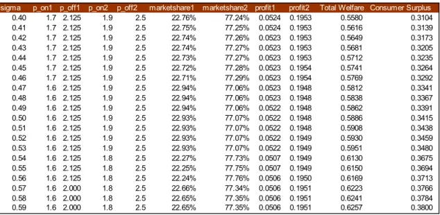
sigma p_on1 p_off1 p_on2 p_off2 marketshare1 marketshare2 profit1 profit2 Total Welfare Consumer Surplus
0.40 1.7 2.125 1.9 2.5 22.76% 77.24% 0.0524 0.1953 0.5580 0.3104 0.41 1.7 2.125 1.9 2.5 22.75% 77.25% 0.0524 0.1953 0.5616 0.3139 0.42 1.7 2.125 1.9 2.5 22.74% 77.26% 0.0523 0.1953 0.5649 0.3173 0.43 1.7 2.125 1.9 2.5 22.74% 77.27% 0.0523 0.1953 0.5681 0.3205 0.44 1.7 2.125 1.9 2.5 22.73% 77.27% 0.0523 0.1953 0.5712 0.3235 0.45 1.7 2.125 1.9 2.5 22.72% 77.28% 0.0523 0.1954 0.5741 0.3264 0.46 1.7 2.125 1.9 2.5 22.71% 77.29% 0.0523 0.1954 0.5769 0.3292 0.47 1.6 2.125 1.9 2.5 22.94% 77.06% 0.0523 0.1948 0.5812 0.3341 0.48 1.6 2.125 1.9 2.5 22.94% 77.06% 0.0523 0.1948 0.5838 0.3367 0.49 1.6 2.125 1.9 2.5 22.94% 77.06% 0.0522 0.1948 0.5862 0.3391 0.50 1.6 2.125 1.9 2.5 22.93% 77.07% 0.0522 0.1948 0.5886 0.3415 0.51 1.6 2.125 1.9 2.5 22.93% 77.07% 0.0522 0.1948 0.5908 0.3438 0.52 1.6 2.125 1.9 2.5 22.93% 77.07% 0.0522 0.1949 0.5930 0.3459 0.53 1.6 2.125 1.9 2.5 22.93% 77.07% 0.0522 0.1949 0.5951 0.3480 0.54 1.6 2.125 1.8 2.5 22.27% 77.73% 0.0507 0.1949 0.6130 0.3675 0.55 1.6 2.125 1.8 2.5 22.25% 77.75% 0.0507 0.1949 0.6150 0.3694 0.56 1.6 2.125 1.8 2.5 22.24% 77.76% 0.0506 0.1950 0.6169 0.3713 0.57 1.6 2.000 1.8 2.5 22.66% 77.34% 0.0506 0.1951 0.6223 0.3766 0.58 1.6 2.000 1.8 2.5 22.65% 77.35% 0.0506 0.1951 0.6241 0.3784 0.59 1.6 2.000 1.8 2.5 22.65% 77.35% 0.0506 0.1951 0.6257 0.3800
Table 5 : Impact of substitutability (competition level)
When substitutability is increased by 50%, neither profit nor market share of two firms show great changes. Consumer surplus, however, is increased by 22.5%. Thus this table justifies the basic idea of fostering competition.
tau p_on1 p_off1 p_on2 p_off2 marketshare1 marketshare2 profit1 profit2 Total Welfare consumer surplus
0.10 1.7 1.875 1.9 2.000 23.92% 76.08% 0.0554 0.1934 0.5033 0.2545 0.11 1.7 1.875 1.9 2.000 23.89% 76.11% 0.0553 0.1935 0.5138 0.2650 0.12 1.7 1.875 1.9 2.125 24.16% 75.84% 0.0550 0.1937 0.5212 0.2725 0.13 1.7 1.875 1.9 2.125 24.08% 75.92% 0.0548 0.1939 0.5317 0.2830 0.14 1.7 2.000 1.9 2.250 23.55% 76.45% 0.0544 0.1942 0.5353 0.2867 0.15 1.7 2.000 1.9 2.250 23.48% 76.52% 0.0542 0.1944 0.5456 0.2970 0.16 1.7 2.000 1.9 2.250 23.40% 76.60% 0.0540 0.1946 0.5559 0.3073 0.17 1.7 2.000 1.9 2.375 23.40% 76.60% 0.0534 0.1948 0.5631 0.3149 0.18 1.7 2.000 1.9 2.375 23.30% 76.70% 0.0532 0.1950 0.5733 0.3251 0.19 1.6 2.125 1.9 2.500 23.03% 76.97% 0.0525 0.1946 0.5784 0.3313 0.20 1.6 2.125 1.9 2.500 22.93% 77.07% 0.0522 0.1948 0.5886 0.3415 0.21 1.6 2.125 1.9 2.625 22.79% 77.21% 0.0515 0.1951 0.5958 0.3492 0.22 1.6 2.125 1.9 2.750 22.61% 77.39% 0.0506 0.1954 0.6031 0.3571 0.23 1.6 2.250 1.9 2.750 22.20% 77.80% 0.0503 0.1955 0.6095 0.3638 0.24 1.6 2.250 1.8 2.875 21.32% 78.68% 0.0479 0.1958 0.6350 0.3912 0.25 1.6 2.250 1.8 3.000 21.05% 78.95% 0.0471 0.1962 0.6431 0.3998 0.26 1.6 2.250 1.8 3.125 20.75% 79.25% 0.0461 0.1967 0.6514 0.4086 0.27 1.5 2.250 1.8 3.250 20.76% 79.24% 0.0452 0.1963 0.6613 0.4197 0.28 1.5 2.375 1.8 3.375 20.31% 79.69% 0.0443 0.1964 0.6663 0.4256 0.29 1.5 2.375 1.8 3.500 19.98% 80.03% 0.0434 0.1969 0.6750 0.4347
Table 6 : Impact of calling externality
Receiving-call’s utility contributes to the reduction of on-net price of both side as well as increase of profit, welfare and consumer surplus.
When beta=0.3,sigma=0.2,gama1=0.1,gama2=0.3,tau=0.1, we show the impact of adjusting the interconnection terminal charge.
a1 p_on1 p_off1 p_on2 p_off2 marketshare1 marketshare2 profit1_by_raising_a1profit2 Total_welfare_raising_a1Customer_surplus_raising_a1
0.70 1.9 2.61 2.0 2.61 22.63% 77.37% 0.0521 0.1941 0.2860 0.0399 0.73 1.9 2.61 2.0 2.66 22.67% 77.33% 0.0524 0.1935 0.2850 0.0391 0.76 1.9 2.61 2.0 2.72 22.71% 77.29% 0.0526 0.1930 0.2841 0.0384 0.79 1.9 2.61 2.0 2.77 22.75% 77.25% 0.0529 0.1926 0.2831 0.0377 0.82 1.9 2.61 2.0 2.83 22.78% 77.22% 0.0531 0.1921 0.2822 0.0371 0.85 1.9 2.61 2.0 2.88 22.82% 77.18% 0.0533 0.1916 0.2813 0.0364 0.88 1.9 2.61 2.0 2.93 22.85% 77.15% 0.0535 0.1912 0.2805 0.0358 0.91 1.9 2.61 2.0 2.99 22.88% 77.12% 0.0536 0.1908 0.2796 0.0352 0.94 1.9 2.61 2.0 3.04 22.92% 77.09% 0.0538 0.1904 0.2788 0.0346 0.97 1.9 2.61 2.0 3.10 22.95% 77.06% 0.0539 0.1900 0.2780 0.0341 1.00 1.9 2.61 2.0 3.15 22.97% 77.03% 0.0541 0.1896 0.2772 0.0335 1.03 1.9 2.61 2.0 3.20 23.00% 77.00% 0.0542 0.1892 0.2764 0.0330 1.06 1.9 2.61 2.0 3.26 23.03% 76.97% 0.0543 0.1889 0.2756 0.0325 1.09 1.9 2.61 2.0 3.31 23.06% 76.95% 0.0544 0.1885 0.2749 0.0320 1.12 1.9 2.61 2.0 3.37 23.08% 76.92% 0.0545 0.1882 0.2742 0.0315 1.15 1.9 2.61 2.0 3.42 23.11% 76.90% 0.0545 0.1879 0.2735 0.0311 1.18 1.9 2.61 1.9 3.47 22.96% 77.04% 0.0542 0.1876 0.2844 0.0427 1.21 1.9 2.61 1.9 3.53 22.98% 77.02% 0.0543 0.1873 0.2837 0.0422 1.24 1.9 2.61 1.9 3.58 23.00% 77.00% 0.0543 0.1870 0.2831 0.0418 1.27 1.9 2.61 1.9 3.64 23.03% 76.97% 0.0544 0.1867 0.2824 0.0414
Table 7 : Impact of raising smaller firm’s terminal access charges
a2 P_on1 p_off1 p_on2 p_off2 marketshare1marketshare2 profit1 profit2 Total_welfare Customer_surplus
0.70 1.9 2.61 2.0 2.61 22.63% 77.37% 0.0521 0.1941 0.2860 0.040 0.67 1.9 2.56 2.0 2.61 22.71% 77.29% 0.0528 0.1936 0.2871 0.041 0.64 1.9 2.50 2.0 2.61 22.79% 77.21% 0.0536 0.1931 0.2882 0.041 0.61 1.9 2.31 2.0 2.61 23.10% 76.90% 0.0544 0.1931 0.2923 0.045 0.58 1.9 2.26 2.0 2.61 23.19% 76.81% 0.0553 0.1924 0.2935 0.046 0.55 1.9 2.21 2.0 2.61 23.29% 76.71% 0.0562 0.1917 0.2947 0.047 0.52 1.9 2.16 2.0 2.61 23.39% 76.61% 0.0572 0.1909 0.2959 0.048 0.49 1.9 2.11 2.0 2.61 23.50% 76.50% 0.0582 0.1900 0.2971 0.049 0.46 1.9 2.06 2.0 2.61 23.61% 76.39% 0.0592 0.1890 0.2984 0.050 0.43 1.9 2.01 2.0 2.61 23.73% 76.27% 0.0604 0.1879 0.2997 0.051 0.40 1.9 1.96 1.9 2.61 23.69% 76.32% 0.0611 0.1867 0.3124 0.065 0.37 1.9 1.90 1.9 2.61 23.82% 76.19% 0.0624 0.1853 0.3137 0.066 0.34 1.9 1.85 1.9 2.61 23.95% 76.05% 0.0637 0.1838 0.3150 0.067 0.31 1.9 1.80 1.9 2.61 24.10% 75.90% 0.0651 0.1822 0.3163 0.069 0.28 1.9 1.75 1.9 2.61 24.25% 75.75% 0.0666 0.1803 0.3176 0.071 0.25 1.9 1.70 1.9 2.61 24.42% 75.58% 0.0682 0.1782 0.3189 0.072 0.22 1.9 1.65 1.9 2.61 24.59% 75.41% 0.0699 0.1759 0.3201 0.074 0.19 1.9 1.60 1.9 2.61 24.78% 75.23% 0.0718 0.1733 0.3214 0.076 0.16 1.9 1.55 1.9 2.61 24.97% 75.03% 0.0738 0.1704 0.3225 0.078 0.13 1.9 1.50 1.9 2.61 25.18% 74.82% 0.0759 0.1670 0.3237 0.081
a1 a2 p_on1 p_off1 p_on2 p_off2 marketshare1 marketshare2 profit1 profit2
0.76 0.25 1.9 1.7 1.9 2.718 24.5% 75.5% 0.06881 0.17713 0.75 0.25 1.9 1.7 1.9 2.700 25.9% 74.1% 0.07249 0.17342 0.74 0.25 1.9 1.8 1.9 2.682 26.9% 73.1% 0.07608 0.17068 0.73 0.25 1.9 1.8 1.9 2.664 27.9% 72.1% 0.07876 0.16803 0.72 0.25 1.9 1.8 1.9 2.646 28.9% 71.1% 0.08137 0.16546 0.71 0.25 1.9 1.8 1.9 2.628 29.9% 70.1% 0.08389 0.16298 0.7 0.25 1.9 1.8 1.9 2.610 30.9% 69.1% 0.08634 0.16058 0.69 0.25 1.9 1.8 1.9 2.592 31.8% 68.2% 0.08872 0.15827 0.68 0.25 1.9 1.8 1.9 2.574 32.7% 67.3% 0.09102 0.15603 0.67 0.25 1.9 1.8 1.9 2.556 33.6% 66.4% 0.09324 0.15387 0.66 0.25 1.9 1.8 1.9 2.679 34.5% 65.5% 0.09462 0.15180 0.65 0.25 1.9 1.8 1.9 2.660 35.4% 64.6% 0.09695 0.14954 0.64 0.25 1.9 1.8 1.9 2.641 36.3% 63.7% 0.09922 0.14736 0.63 0.25 1.9 1.8 1.9 2.622 37.2% 62.8% 0.10140 0.14525 0.62 0.25 1.9 1.8 1.9 2.603 38.1% 61.9% 0.10352 0.14322 0.61 0.25 1.9 1.8 1.9 2.584 38.9% 61.1% 0.10557 0.14126 0.6 0.25 1.9 1.8 1.9 2.565 39.8% 60.3% 0.10755 0.13937 0.59 0.25 1.9 1.8 1.9 2.546 40.5% 59.5% 0.10947 0.13755 0.58 0.25 1.9 1.9 1.9 2.527 41.1% 58.9% 0.11132 0.13627 0.57 0.25 1.9 1.9 1.9 2.508 41.7% 58.3% 0.11265 0.13503 0.56 0.25 1.9 1.9 1.9 2.489 42.3% 57.7% 0.11394 0.13384 0.55 0.25 1.9 1.9 1.9 2.470 42.8% 57.2% 0.11518 0.13270 0.54 0.25 1.9 1.9 1.9 2.451 43.3% 56.7% 0.11636 0.13161 0.53 0.25 1.9 1.9 1.9 2.432 43.9% 56.1% 0.11750 0.13057 0.52 0.25 1.9 1.9 1.9 2.413 44.4% 55.6% 0.11858 0.12958 0.51 0.25 1.9 1.9 1.9 2.394 44.8% 55.2% 0.11962 0.12864 0.5 0.25 1.9 1.9 1.9 2.375 45.3% 54.7% 0.12060 0.12775 0.49 0.25 1.9 1.9 1.9 2.356 45.7% 54.3% 0.12153 0.12690 0.48 0.25 1.9 1.9 1.9 2.337 46.2% 53.8% 0.12242 0.12611 0.47 0.25 1.9 1.9 1.9 2.318 46.6% 53.4% 0.12325 0.12536 0.46 0.25 1.9 1.9 1.9 2.299 47.0% 53.0% 0.12403 0.12466 0.45 0.25 1.9 1.9 1.9 2.280 47.3% 52.7% 0.12476 0.12401 0.44 0.25 1.9 1.9 1.9 2.261 47.7% 52.3% 0.12544 0.12341 0.43 0.25 1.9 1.9 1.9 2.242 48.1% 51.9% 0.12606 0.12286 0.42 0.25 1.9 1.9 1.9 2.223 48.4% 51.6% 0.12663 0.12236 0.41 0.25 1.9 1.9 1.9 2.204 48.7% 51.3% 0.12715 0.12191 0.4 0.25 1.9 1.9 1.9 2.185 49.0% 51.0% 0.12761 0.12151 0.39 0.25 1.9 1.9 1.9 2.166 49.3% 50.7% 0.12802 0.12115 0.38 0.25 1.9 1.9 1.9 2.147 49.5% 50.5% 0.12837 0.12085 0.37 0.25 1.9 1.9 1.9 2.128 49.7% 50.3% 0.12866 0.12061 0.36 0.25 1.9 1.9 1.9 2.109 50.0% 50.0% 0.12890 0.12041
a1 a2 p_on1 p_off1 p_on2 p_off2 marketshare1 marketshare2 profit1 profit2
0.885 0.30 1.9 1.785 1.9 2.943 24.37% 75.63% 0.0671 0.1785 0.870 0.30 1.9 1.785 1.9 2.916 25.63% 74.37% 0.0704 0.1752 0.855 0.30 1.9 1.89 1.9 2.889 26.57% 73.43% 0.0737 0.1725 0.840 0.30 1.9 1.89 1.9 2.862 27.49% 72.51% 0.0761 0.1702 0.825 0.30 1.9 1.89 1.9 2.835 28.38% 71.62% 0.0784 0.1679 0.810 0.30 1.9 1.89 1.9 2.808 29.25% 70.75% 0.0806 0.1658 0.795 0.30 1.9 1.89 1.9 2.781 30.10% 69.90% 0.0828 0.1637 0.780 0.30 1.9 1.89 1.9 2.754 30.93% 69.07% 0.0849 0.1617 0.765 0.30 1.9 1.89 1.9 2.727 31.73% 68.27% 0.0869 0.1597 0.750 0.30 1.9 1.89 1.9 2.700 32.51% 67.49% 0.0889 0.1579 0.735 0.30 1.9 1.89 1.9 2.673 33.26% 66.74% 0.0908 0.1561 0.720 0.30 1.9 1.89 1.9 2.793 34.09% 65.91% 0.0918 0.1545 0.705 0.30 1.9 1.89 1.9 2.765 34.90% 65.10% 0.0938 0.1526 0.690 0.30 1.9 1.89 1.9 2.736 35.68% 64.32% 0.0957 0.1508 0.675 0.30 1.9 1.89 1.9 2.708 36.44% 63.56% 0.0975 0.1491 0.660 0.30 1.9 1.89 1.9 2.679 37.18% 62.82% 0.0993 0.1475 0.645 0.30 1.9 1.89 1.9 2.651 37.89% 62.11% 0.1010 0.1459 0.630 0.30 1.9 1.89 1.9 2.622 38.58% 61.42% 0.1026 0.1444 0.615 0.30 1.9 1.89 1.9 2.594 39.25% 60.75% 0.1042 0.1430 0.600 0.30 1.9 1.89 1.9 2.565 39.90% 60.11% 0.1057 0.1417 0.585 0.30 1.9 1.89 1.9 2.537 40.52% 59.49% 0.1071 0.1405 0.570 0.30 1.9 1.995 1.9 2.508 40.94% 59.06% 0.1084 0.1394 0.555 0.30 1.9 1.995 1.9 2.480 41.35% 58.65% 0.1092 0.1388 0.540 0.30 1.9 1.995 1.9 2.451 41.73% 58.27% 0.1100 0.1381 0.525 0.30 1.9 1.995 1.9 2.423 42.09% 57.91% 0.1107 0.1376 0.510 0.30 1.9 1.995 1.9 2.394 42.44% 57.57% 0.1113 0.1371 0.495 0.30 1.9 1.995 1.9 2.366 42.75% 57.25% 0.1118 0.1367 0.480 0.30 1.9 1.995 1.9 2.337 43.05% 56.95% 0.1123 0.1364 0.465 0.30 1.9 1.995 1.9 2.309 43.32% 56.68% 0.1127 0.1361 0.450 0.30 1.9 1.995 1.9 2.280 43.58% 56.43% 0.1130 0.1359 0.435 0.30 1.9 1.995 1.9 2.252 43.80% 56.20% 0.1132 0.1358 0.420 0.30 1.9 1.995 1.9 2.223 44.00% 56.00% 0.1134 0.1357 0.405 0.30 1.9 1.995 1.9 2.195 44.18% 55.82% 0.1135 0.1358 0.390 0.30 1.9 1.995 1.9 2.166 44.33% 55.67% 0.1134 0.1359 0.375 0.30 1.9 1.995 1.9 2.138 44.45% 55.55% 0.1133 0.1361 0.360 0.30 1.9 1.995 1.9 2.109 44.55% 55.45% 0.1131 0.1363 0.345 0.30 1.9 1.995 1.9 2.081 44.62% 55.39% 0.1128 0.1367 0.330 0.30 1.9 1.995 1.9 2.052 44.65% 55.35% 0.1124 0.1371 0.315 0.30 1.9 1.995 1.9 2.024 44.66% 55.34% 0.1119 0.1377 0.300 0.30 1.9 1.995 1.9 1.995 44.64% 55.36% 0.1112 0.1383
a1 a2 p_on1 p_off1 p_on2 p_off2 marketshare1 marketshare2 profit1 profit2
0.87 0.3 1.9 1.785 1.9 2.916 24.35% 75.65% 0.0670 0.1787 0.84 0.3 1.9 1.785 1.9 2.862 25.58% 74.42% 0.0702 0.1757 0.81 0.3 1.9 1.89 1.9 2.808 26.47% 73.53% 0.0732 0.1734 0.78 0.3 1.9 1.89 1.9 2.754 27.32% 72.68% 0.0753 0.1715 0.75 0.3 1.9 1.89 1.9 2.700 28.13% 71.88% 0.0773 0.1697 0.72 0.3 1.9 1.89 1.9 2.646 28.89% 71.11% 0.0791 0.1681 0.69 0.3 1.9 1.89 1.9 2.592 29.61% 70.39% 0.0808 0.1667 0.66 0.3 1.9 1.89 1.9 2.538 30.29% 69.71% 0.0823 0.1654 0.63 0.3 1.9 1.89 1.9 2.484 30.92% 69.08% 0.0837 0.1643 0.60 0.3 1.9 1.89 1.9 2.430 31.50% 68.50% 0.0848 0.1634 0.57 0.3 1.9 1.89 1.9 2.376 32.04% 67.97% 0.0859 0.1626 0.54 0.3 1.9 1.89 1.9 2.451 32.63% 67.37% 0.0861 0.1620 0.51 0.3 1.9 1.89 1.9 2.394 33.18% 66.82% 0.0871 0.1613 0.48 0.3 1.9 1.89 1.9 2.337 33.67% 66.33% 0.0878 0.1607 0.45 0.3 1.9 1.89 1.9 2.280 34.11% 65.89% 0.0884 0.1604 0.42 0.3 1.9 1.89 1.9 2.223 34.50% 65.50% 0.0887 0.1603 0.39 0.3 1.9 1.89 1.9 2.166 34.83% 65.18% 0.0889 0.1603 0.36 0.3 1.9 1.89 1.9 2.109 35.09% 64.91% 0.0887 0.1606 0.33 0.3 1.9 1.89 1.9 2.052 35.30% 64.70% 0.0883 0.1610 0.30 0.3 1.9 1.89 1.9 1.995 35.44% 64.56% 0.0877 0.1617
Table 11 : Dynamic regulation 20 periods
a1 a2 p_on1 p_off1 p_on2 p_off2 marketshare1 marketshare2 profit1 profit2
0.84 0.3 1.9 1.785 1.9 2.862 24.32% 75.68% 0.0668 0.1792 0.78 0.3 1.9 1.785 1.9 2.754 25.48% 74.52% 0.0696 0.1768 0.72 0.3 1.9 1.89 1.9 2.646 26.26% 73.74% 0.0721 0.1753 0.66 0.3 1.9 1.89 1.9 2.538 26.95% 73.05% 0.0735 0.1744 0.60 0.3 1.9 1.89 1.9 2.430 27.55% 72.45% 0.0745 0.1738 0.54 0.3 1.9 1.89 1.9 2.322 28.06% 71.94% 0.0750 0.1737 0.48 0.3 1.9 1.89 1.9 2.214 28.45% 71.55% 0.0751 0.1740 0.42 0.3 1.9 1.89 1.9 2.106 28.73% 71.27% 0.0746 0.1747 0.36 0.3 1.9 1.89 1.9 1.998 28.89% 71.12% 0.0734 0.1760 0.30 0.3 1.9 1.89 2 1.890 29.05% 70.95% 0.0719 0.1778