Understanding the Fine Structure of Electricity Prices
HÉLYETTE GEMAN
University Paris Dauphine
& ESSEC Business School
ANDREA RONCORONI
ESSEC Business School
& Bocconi University
Abstract
This paper analyzes the special features of electricity spot prices derived from the physics of this commodity and from the economics of supply and demand in a market pool. Besides mean-reversion, a property they share with other commodities, power prices exhibit the unique feature of spikes in trajectories. We introduce a class of discontinuous processes exhibiting a ”jump-reversion” component to properly represent these sharp upward moves shortly followed by drops of similar magnitude. Our approach allows to capture - for the first time to our knowledge - both the trajectorial and the statistical properties of electricity pool prices. The quality of the fitting is illustrated on a database of major US power markets.
We wish to thank Alexander Eydeland for helpful comments on an earlier version of this paper. All remaining errors are ours.
Understanding the Fine Structure of Electricity Prices
Abstract
This paper analyzes the special features of electricity spot prices derived from the physics of this commodity and from the economics of supply and demand in a market pool. Besides mean-reversion, a property they share with other commodities, power prices exhibit the unique feature of spikes in trajectories. We introduce a class of discontinuous processes exhibiting a ”jump-reversion” component to properly represent these sharp upward moves shortly followed by drops of similar magnitude. Our approach allows to capture - for the first time to our knowledge - both the trajectorial and the statistical properties of electricity pool prices. The quality of the fitting is illustrated on a database of major US power markets.
I. Introduction
A decade ago, the electricity sector worldwide was a vertically integrated industry where prices were set by regulators and reflected the costs of generation, transmis-sion and distribution. In this setting, power prices used to change rarely, and in an essentially deterministic manner. Over the last ten years, major countries have been experiencing deregulation in generation and supply activities (transmission, and even more so, distribution activities generally remaining under the state authority). One of the important consequences of this restructuring is that prices are now determined according to the fundamental economic rule of supply and demand. Supply is pro-vided by generators and demand is represented by industrial consumers and power marketers buying electricity in the pool to sell it to end-users. There is a ”market pool” where bids placed by generators to sell electricity for the next day are con-fronted to purchase orders and equilibrium prices are defined as the intersection of the aggregate demand and supply curves for each hour (or half-hour) in the day.
In a parallel way, deregulation of the energy industry has paved the way for a considerable amount of trading activity, both in the spot and derivative markets. It has provided utilities with new opportunities but challenges as well. The volume risk they have been used to analyze and account for in their revenue projections is now augmented by price risk. This price risk has forced the industry to go into financial practices such as hedging, use of derivatives and, quite importantly, to identify and
price the options embedded in energy contracts that have been written for decades. Accordingly, the scheduling of plant operation and maintenance has become the sub-ject of even increased scrutiny and concern.
In contrast to stocks and bonds, electricity prices are affected by transmission constraints, seasonality, weather, by the nature of the generation stack and the non-storability constraint (outside hydro). An implication of these specific features is that electricity prices are much more likely to be driven by spot demand and supply considerations than other commodities, with demand in the short-term market being fairly inelastic. As a result, sizeable shocks in production or consumption may give rise to the price jumps which have been observed since 1998 in various parts in the United States. Leaving aside the California 2000 events which were possibly driven by flaws in market design and wrongdoings on the part of some major players, spike prices have been motivated by disruption in transmission, generation outages, extreme weather or a conjunction of these circumstances.
Today, an important fraction of the literature on electricity belongs to the eco-nomics and industrial ecoeco-nomics arena, and analyzes deregulated electricity markets from the regulatory and industrial organization viewpoints (see for instance Joskow and Kahn (1999)). It is clear that in the understanding of the behavior of electricity prices, economics, finance and physics all come into play; a proper mathematical rep-resentation of spot prices is however a necessary exercise and the cornerstone for the
optimal scheduling of physical assets, the valuation of financial and real options and more generally the risk management of utilities and energy companies. For instance, volumetric options granted in traditional energy contracts or traded as individual financial instruments crucially depend on the spot price of electricity at any date during the lifetime of the option.
Some initial papers on the modeling of power price processes include Deng (1999), Bhanot (2000), Barone-Adesi and Gigli (2002), Lucia and Schwartz (2000), Knittel and Roberts (2001), Barlow (2002), Escribano et al. (2002). We extend this litera-ture by proposing a family of stochastic processes meant to represent the trajectorial and statistical features displayed by electricity spot prices in deregulated power mar-kets. We also introduce an effective method to identify spikes in historical raw data. In order to empirically investigate the information content of observed power price dynamics, we design a procedure for best fitting our model to market data both in terms of trajectories and moments. Since our focus is an analysis of electricity prices in terms of the appropriate mathematical process representing them (as well as the parameters attached to it), we shall solely work under the physical probability mea-sure. Yet, our concern is to preserve the Markov property in the view of developments on standard and exotic derivatives valuation.
The outline of the paper is as follows. Section II discusses the main features of power prices and of the stack function. Section III introduces a class of processes that
may encompass prices observed in a variety of regional markets. Section IV contains the description of data for three major U.S. power markets which exhibit different degrees of mean-reversion and spike behavior. Section V analyzes the appropriate statistical methods to select a process within the proposed class in order to match ob-served spot prices. Alternative model specifications are also discussed in that section. Section VI presents empirical results for all models and markets under investigation. Section VII concludes with a few comments and suggestions for future research.
II. The Key Features of Power Prices
Most of the important literature on commodities has focused on storable commodities (see for instance Fama and French (1987)). The same property applies to the specific case of energy commodities (oil being the fundamental example), since deregulated power markets were established fairly recently. Moreover, whether it includes electric-ity or not, most of the important research has focused on forward curves: Litzenberger and Rabinovitz (1995) document that nine-month oil futures prices are below the one-month prices 77% of the time, i.e., that oil forward curves are mostly ”backwardated”. Routledge, Seppi and Spatt (2000) propose an equilibrium term structure of forward prices for storable commodities and show that these forward curves differ from those for stocks and bonds because of the timing option attached to the ownership of the physical goods in inventory. Bessembinder and Lemmon (2002) build directly an
equi-librium model for electricity forward markets derived from optimal hedging strategies conducted by utilities (power marketers, speculators and other types of market par-ticipants not being incorporated in the equilibrium analysis). They compare in this setting forward prices to future spot prices and show that the former are downward-biased estimators of the latter if expected demand is low and demand risk is moderate; in contrast the forward premium increases when either expected demand or demand risk is high, because of the positive skewness in the spot power price distribution. These results are quite instructive since in power markets, like in any other com-modity markets, the validity of the representation of forward prices as expectations of future spot prices is a matter of interest for all participants. Geman and Vasicek (2001) empirically confirm Bessembinder and Lemmon’s findings and demonstrate, on a U.S. database, that short-term forward contracts are upward biased estimators of future spot prices, in agreement with the high volatility and risk attached to U.S. spot power markets.
Our perspective in this paper is complementary and distinct at several levels. Firstly, we are interested in the modeling of the spot price of electricity, since we believe that in the wake of deregulation of power markets, a proper representation of the dynamics of spot prices becomes a necessary tool for trading purposes and optimal design of supply contracts. As discussed in Eydeland and Geman (1998), the non-storability of electricity implies the breakdown of the spot-forward relationship
and, in turn, the possibility of deriving in an equilibrium approach the fundamental properties of spot prices from the analysis of forward curves. Moreover, as may be exhibited empirically in markets as different as the Nordpool, the U.K. or the U.S., electricity forward curve moves are much less dramatic than spot price changes, in agreement with the less stringent constraints of future delivery.
If we turn to the wide literature dedicated to commodity prices in general, we observe that the convenience yield plays an important role in many cases. The in-teresting concept of convenience yield (possibly defined as net of storage costs) was introduced for agricultural commodities in the seminal work by Kaldor (1939) and Working (1949). It is meant to represent the benefit from holding the commodity, either to meet unexpected demand and avoid production interruption or to unwind a forward or a derivative contract. This benefit accrues for the holder of the com-modity and not to the owner of a forward contract. More recently, Schwartz (1997) has included in the modeling of oil prices a stochastic convenience yield and derived option prices in this framework. Beyond the difficulties posed by the introduction in a model of such a non-observable risk factor, our view is that a convenience yield does not really make sense in the context of electricity: since there is no available technique to store power (outside of hydro), there cannot be a benefit from holding the commodity, nor a storage cost. Hence, the spot price process should contain by itself most of the fundamental properties of power, as listed below.
A first characteristic of electricity (and other commodity) prices is mean reversion toward a level that represents marginal cost and may be constant, periodic or periodic with a trend. In contrast, when looking at equity price modelling, the financial literature has classically introduced an average growth of the stock price depicted by the drift term of the geometric Brownian motion. This is fully consistent with such models as the Capital Asset Pricing Model which express the fact that the stock buyer expects to receive on her investment the risk-free rate as well as a risk premium. Results of similar studies conducted for commodities are quite different, confirming that commodities are not assets. Pyndick (1999) analyzes a 127-year period for crude oil and bituminous coal and a 75-year period for natural gas. He concludes that prices deflated (and represented by their natural logarithms), exhibit mean-reversion to a stochastically fluctuating trend line. In the case of power and with a few years horizon in mind, we propose to represent the diffusion part of the price process as mean-reverting to a deterministic periodical trend driven by seasonal effects. This periodicity in the trend reflects the average consumption levels of electricity across the year and highly depends on climatological conditions in the specific region of analysis (as we shall see, the mean reversion will be more or less pronounced in different markets). Therefore, we will consider the periodic feature as a predictable component of the random evolution of power prices.
ran-dom moves around the average trend, which represent the temporary supply/demand imbalances in the network. This effect is locally unpredictable and may be represented by a white noise term affecting daily price variations.
A third and intrinsic feature of power price processes is the presence of so-called spikes, namely one (or several) upward jumps shortly followed by a steep downward move, for instance when the heat wave is over or the generation outage resolved. Since shocks in power supply and demand cannot be smoothed away by inventories, our view is that these spikes are not necessarily due to poor market design and will persist beyond the transition phase of power deregulation. The California situation has been widely discussed over the last two years by economists as well as in daily newspapers, but many studies neglect to mention that the first event of this nature was totally unrelated to the possible exercise of market power by some key providers: in the ECAR region (covering several Midwestern states of the U.S.A.), prices in June 1998 went to several thousand dollars up from 25 dollars per megawatthour. This spectacular rise was due to the conjunction of a long heat wave, congestion in transmission of hydroelectricity coming from Canada and production outage of a nuclear plant hit by a tornado. Within two days, prices fell back to a 50 dollars range as the weather cooled down and transmission capacity was restored. It is interesting to observe that, despite the magnitude of the spike (the highest observed so far), the system in ECAR as well as neighboring regions did not collapse; only some companies
which had sold electricity options without fully envisioning the risks involved went bankrupt.
It is clear that the continuous balance between supply and demand by the operator of a bulk power network may fail more than momentarily under extreme contingen-cies. For instance in Europe, where weather events are usually less dramatic than in the U.S. (and capacity reserves probably higher), prices went from 25 to 500 Euros on the Leipzig Exchange (now European Energy Exchange) for a few days after a long cold spell in December 2001. From an economic standpoint, this phenomenon is illuminated by the graph of the marginal cost of electricity supply, called power stack function (see Eydeland and Geman (1998)). Knowing the characteristics of the different plants in a given region, we can calculate the marginal cost of generation for all units. By stacking the units in ”merit order”, i.e., from the lowest to the highest cost, we can build what is called a supply stack or a stack function. The marginal cost of a given generator depends in fact not only on current fuel costs but also on the previous states of the unit in terms of outages or scheduled maintenance. Leaving the fine details aside (such as unplanned outages), the stack function can be built by considering only the marginal fuel costs and variable operation and main-tenance (O&M) costs. The baseload part which is taken care of by low cost plants (coal-fired or hydro-activated) starts being flat or with a small upward slope; then the curve reaches a point where there is an exponential increase corresponding to very
expensive units such as ”peakers” being activated.
Figure 1 represents the merit order stack for the ECAR region. As in all com-petitive markets, electricity prices are determined by the intersection point of the aggregate demand and supply functions. A forced outage of a major power plant or a sudden surge in demand due to extreme weather conditions would either shift the supply curve to the left or lift up the demand curve, causing in both cases a price jump. When climate returns to normal and/or other generation units come into play, the price quickly falls down to the normal range, generating the characteristic spike in the trajectory. These spikes are obviously a major subject of concern for practitioners who need to honor their supply contracts at all times. Consequently, they are the subject of a careful analysis; as for the construction of the stack function, it repre-sents an important component of the so-called ”fundamental” approach to electricity prices.
Figure 1 about here
Following the jump-diffusion model proposed in 1976 by Merton to account for dis-continuities in stock price trajectories, a number of authors have introduced a Poisson component to represent the large upward moves of electricity prices; then, the ques-tion of bringing prices down needs to be solved. Deng (1999) introduces a sequential regime-switching representation which may be a good way of addressing the dramatic changes in spot prices; the trajectories produced by the model are however fairly
different from the ones observed in the market.
Lucia and Schwartz (2000) examine the Nordpool market and choose not to in-troduce any jump component in the price process. Data from this market shows that despite the significant part of hydroelectricity in the northern part of Europe, power prices do not have continuous trajectories; for instance, there is a quasi-yearly violent downward jump early April at the end of the snow season when uncertainty about reservoir levels is resolved. This tends to support our view that jump components are hard to avoid when modelling power prices, since they are structurally related to the physical features of this commodity. The class of models presented below is meant to translate the fact that there are several regimes for electricity prices, corresponding respectively to the quasi-flat and sharply convex parts of the merit order stack. Under the normal regime, the aggregate capacity of generation in the region under analysis is sufficient to meet consumer demand. In this regime, price fluctuations are driven by shifts in consumer demand and shifts in the marginal costs (e.g., fuel) of the marginal power provider. However, when shocks are extreme, a turbulent regime emerges since some utilities or other power distributors may default on their deliveries. Because the demand of each utility for electricity to service consumers’ needs is inelastic until all financial reserves have been exhausted, spot prices will rise high enough to absorb these reserves, which may lead to large spikes. Once the demand shock is passed, prices fall back to the normal fluctuation pattern. We can observe that in the case of
storable commodities (such as oil or wheat), prices are determined not only by supply from existing production and demand for current consumption, but also by the level of inventories. The buffering effect of these inventories does not exist in the case of electricity (except to some extent for hydro).
This paper aims to provide a reliable and flexible representation for the random behavior of power prices. We argue that the classical setting of continuous-path diffusion processes does not deliver a viable solution to this problem for reasons linked to trajectories as well as statistical features of daily power price returns. A jump component may account for the occurrence of spikes through an appropriate jump-intensity function and also explain the significant deviations from normality in terms of high order moments observed in logarithmic prices. Figure 2 compares as an example the empirical distribution in the ECAR market to a normal density with the same mean and variance.
Figure 2 about here
We now turn to the construction of a family of processes capable of reproducing the fundamental features of trajectorial and statistical features of power prices.
III. The Model
We model the behavior of the price process of one megawatthour of electricity traded in a given pool market.1 In order to ensure strict positivity of prices and enhance the robustness of the calibration procedure, we represent the electricity spot price in nat-ural logarithmic scale.2 Throughout the paper, except for the pictures representing trajectories, the term price will refer to ”log-price”.
The spot price process is represented by the (unique) solution of a stochastic differential equation of the form:
dE (t) = Dµ (t) dt + θ1
£
µ (t) − E¡t−¢¤dt + σdW (t) + h¡t−¢dJ (t) , (1)
where D denotes the standard first order derivative and f (t−) stands for the left limit of f at time t.
The deterministic function µ (t) represents the predictable seasonal trend of the price dynamics around which spot prices fluctuate. The second term ensures that any shift away from the trend generates a smooth reversion to the average level µ (t). The positive parameter θ1 represents the average variation of the price per unit of shift
away from the trend µ (t) per unit of time. Note that the speed of mean-reversion depends on the current electricity price level since the constant θ1 is multiplied by
µ (t) − E (t−), a difference that may be quite large in electricity markets (in contrast
present). The process W is a (possibly n-dimensional) standard Brownian motion representing unpredictable price fluctuations and is the first source of randomness in our model. The constant σ defines the volatility attached to the Brownian shocks. Note that the instantaneous squared volatility of prices is represented by the condi-tional second order moment of absolute price variations over an infinitesimal period of time: in the present context, it is the sum of the squared Brownian volatility and a term generated by the jump component (see for instance Gihman and Skorohod (1972)).
The discontinuous part of the process reproduces the effect of periodically recur-rent spikes. A spike is a cluster of upward shocks of relatively large size with respect to normal fluctuations, followed by a sharp return to normal price levels. We repre-sent this behavior by assigning a level-dependent sign for the jump component. If the current price is below some threshold, prices are in the normal regime and any forth-coming jump is upward directed. If instead, the current price is above the threshold, the market is experiencing a period of temporary imbalance between demand and supply reflected by abnormally high prices and upcoming jumps are expected to be downward directed.
Jumps are characterized by their time of occurrence, size and direction. The jump times are described by a counting process N (t) specifying the number of jumps experienced up to time t. There exists a corresponding intensity process ι defining the
instantaneous average number of jumps per time unit. We choose for ι a deterministic function that we write as:
ι (t) = θ2× s (t) , (2)
where s (t) represents the normalized (and possibly periodic) jump intensity shape and the constant θ2 can be interpreted as the maximum expected number of jumps
per time unit.
The jump sizes are modeled as increments of a compound jump process J (t) = PN (t)
i=1 Ji. Here the Ji’s are independent and identically distributed random variables
with common density:
p (x; θ3, ψ) = c (θ3) × exp (θ3f (x)) , 0 ≤ x ≤ ψ, (3)
where c (θ3) is a constant ensuring that p is a probability distribution density and ψ
is the maximum jump size. The choice of a truncated density within the exponential family is meant to properly reproduce the observed high order moments.
The jump direction determines the algebraic effect of a jump size Ji on the power
price level. It is represented by a function h, taking values +1 and −1 according to whether the spot price E (t) is smaller or greater than a threshold T :
h (E (t)) = +1 if E (t) < T (t) −1 if E (t) ≥ T (t) . (4)
This function plays an important role in our model for two sets of reasons related to the trajectorial properties of the process and the descriptive statistics of daily price returns (see Roncoroni (2002)). Some authors have proposed to model spikes by introducing large positive jumps together with a high speed of mean reversion; in particular Deng (1999) who was among the first ones to address the specific features of electricity prices. However, models with upward jumps only are deemed to display a highly positive skewness in the price return distribution, in contrast to the one observed in the markets. Other authors model spikes by allowing signed jumps (for instance Escribano et al. (2002)), but if these jumps randomly follow each other, the spike shape has obviously a very low probability to be generated. Lastly, another type of solution proposed in particular by Huisman and Mahieu (2001) and Baroni-Adesi and Gigli (2002), is the introduction of a regime-switching model. This representation does not allow the existence of successive upward jumps; moreover, a return to normal levels through a sharp downward jump would require in this case a non Markovian specification. As a consequence, calibrating a regime-switching model is often quite problematic.
In our setting a proper choice of the barrier T coupled with a high jump intensity can generate a sequence of upward jumps leading to high price levels, after which a discontinuous downward move together with the smooth mean reversion brings prices down to a normal range. Moreover, our representation has the merit of preserving
the Markov property in a single state variable.
Let us observe that general results about stochastic differential equations of the proposed type ensure that equation (1) admits a unique solution (see Gihman and Skorohod (1972)). Hence, the level dependent signed-jump model with time-varying intensity is fully described.
IV. Electricity Data Set
We calibrate the model on a data set consisting of a series of 750 daily average prices compiled from the publication Megawatt Daily for three major U.S. power markets: COB (California Oregon Border), PJM (Pennsylvania-New Jersey-Maryland) and ECAR (East Center Area Reliability coordination agreement). These markets may be viewed as representative of most U.S. power markets both because of their various locations (California, East Coast and Midwestern), because of the different mix of generation (for instance, an important share of hydroelectricity in California) and lastly because of the type of transmission network servicing the region. Moreover, the market design in ECAR and PJM has proved to have functioned properly so far; the choice of the period of analysis (ending in 1999) was meant to leave aside the California crisis and its effects on the COB pool. In terms of price behavior, the COB market is typical of ”low-pressure” markets (such as Palo Verde, Mid Columbia, and Four Corners), with high prices ranging between $90 and $115 per megawatthour in
the examined period. The PJM market represents a ”medium-pressure” market (such as West New York, East New York, and Ercott) with highs between $263 and $412 per megawatthour during that period. Lastly, the ECAR market portrays ”high-pressure” markets (such as MAAP, Georgia-Florida Border, North SPP, South SPP and MAIN), experiencing spikes between 1, 750 and 2, 950 dollars per megawatthour. Figures 3 to 5 depict absolute historical price paths in these markets for the period between January 6, 1997 and December 30, 1999.
Figures 3, 4, and 5 about here
As stated earlier, our goal is to adjust our class of processes to both trajectorial features (i.e., average trend, Brownian volatility, periodical component and spikes) and statistical features (i.e., mean, variance, skewness and kurtosis of daily price returns) of historical prices.
In order to start the calibration procedure, we need to detect jumps in the raw market data. The estimation of a mixed jump-diffusion over a discrete sequence E= (E1, ..., En) of observations may result in an ill-posed problem: standard methods
in statistical inference require samples to represent whole paths over a time interval. In the case of discretely sampled observations, there are infinitely many ways a given price variation over a discrete time interval can be split into an element stemming from the continuous part of the process and another from the discontinuous one. Hence, the problem of disentangling these two components on a discrete sample cannot be
resolved in a theoretically conclusive way; yet, the situation is better in a continuous time representation, which is our case. All examined data exhibit excess of kurtosis in the empirical distribution of daily price variations. These changes tend to cluster close to either their average mean or to the largest observed values (see Figure 2). In other words, data suggests that either there is a jump, in which case the variation due to the continuous part of the process is negligible, or there is no jump and the price variation is totally generated by the continuous part of the process. This observation leads us to identify a price change threshold Γ allowing one to discriminate between the two situations. In this order, we extract from the observed data set two important elements of the calibration procedure: the set ∆Ed of sampled jumps
and the ”Γ-filtered” continuous sample path Ec obtained by juxtaposition of the continuous variations starting at the initial price.3 A discussion of possible selection schemes in a general mathematical setting may be found in Yin (1988). We include Γ as a parameter to be estimated within the calibration procedure: for each market under investigation, we perform our calibration procedure over different ”Γ-filtered” data sets for values of Γ chosen in the set of observed daily price variations. Then, we select the value of Γ leading to the best calibrated model in view of its ability to match descriptive statistics of observed daily price variations. From now on, we suppose a value for Γ has been identified for the market under analysis and input data is described by the corresponding ”Γ-filtered” pair¡Ec, ∆Ed¢.
V. Calibration
We propose a two-step calibration procedure. A first step is the assignment of a specific form for the ”structural” elements in the dynamics described in equation (1) and defined as:
• the mean trend µ (t),
• the jump intensity shape s (t),
• the threshold T defining the sign of the jump • the jump size distribution p (x).
These quantities translate into path properties of the price process.
A second step consists in statistically estimating the four parameters of the se-lected model, namely:
• the mean reversion force θ1,
• the jump intensity magnitude θ2,
• the jump size distribution parameter θ3,
The resulting parametric model is fit to the filtered prices by a new statistical method described further on and based on likelihood estimation for continuous-time processes with discontinuous sample paths.
We now illustrate the implementation of this calibration procedure for the ECAR market, propose possible alternatives to the resulting model and defer results and comments to the next section.
A. Selection of the Structural Elements
The mean trend µ (t) can be determined by fitting an appropriate parametric family of functions to the data set. As mentioned earlier, power prices exhibit a weak sea-sonality in the mean trend and a sharper periodicity in the occurrence of turbulences across the year. The latter periodicity may be an effective estimate for the one dis-played by mean trend: for instance, ECAR market data shows price pressure once a year, during warm season. Some markets display price pressure twice a year, with winter average prices lower than summer average prices (which requires a lower local maximum in the former case). In general, we find that a combination of an affine function and two sine functions with respectively a 12-month and a 6-month period-icity, is appropriate for the U.S. historical data under investigation. We accordingly define the mean trend by a parametric function:
The first term may be viewed as a fixed cost linked to the production of power. The second one drives the long run linear trend in the total production cost. The overall effect of the third and fourth terms is a periodic path displaying two maxima per year, of possibly different magnitudes. Observed prices over the three-year period are averaged into a one-year period and bounded from above by a suitable quantile ν of their empirical distribution. The trend function µ is fitted to the resulting average data by a sequential OLS method providing parameters α, β, γ, δ, ε, and ζ.
We now turn to the identification of the jump intensity shape s. Since spikes occur over short time periods, we select an intensity function exhibiting pronounced convex peaks with annual periodicity. This is meant to reflect the shape of the power stack function which, as shown in Figure 1, becomes very convex (and quasi vertical) at some demand level. Sharp convexity also ensures that the price jump occurrence tends to cluster around the peak dates and rapidly fades away. In this order we choose: s (t) = · 2 1 + |sin [π (t − τ) /k]|− 1 ¸d . (6)
Here the jump occurrence exhibits peaking levels at multiples of k years, beginning at time τ .4 For instance, price shocks concentrating twice a year at evenly spaced dates, with a maximum on August 1, are recovered by the choice τ = 7/12 and k = 1/2. The exponent d allows to adjust the dispersion of jumps around peaking times and is
included among parameters to be estimated within the calibration procedure. Figure 6 shows intensity functions across different coefficients d and Figure 7 reports a sample of jump times.
Figure 6 about here
Figure 7 about here
We found that in all three examined market the best value for d is 2. We have discussed earlier the introduction of a barrier T above which all occurring jumps are downward directed. This threshold may reasonably be defined by a constant spread ∆ over the selected average trend:
T (t) = µ (t) + ∆. (7)
The choice of ∆ results from a balance between two competing effects: the greater the value of ∆, the higher the level power prices may reach during pressure periods; the smaller this value, the sooner the downward jump effect toward normal levels. Equally importantly, this choice has an impact on the moments of daily price variations; indeed, a large value of ∆ induces a noticeably positive skewness.
The last structural element to be determined is a probability distribution for the jump size. We select a truncated version of an exponential density with parameter
θ3:
p (x; θ3, ψ) =
θ3exp (−θ3x)
1 − exp (−θ3ψ)
, 0 ≤ x ≤ ψ, (8)
where ψ represents an upper bound for the absolute value of price changes. This distri-bution belongs to the family described in equation (3), where c (θ3) = θ3/ (1 − exp (−θ3ψ))
and f (x) = −x. The resulting price process is a ”special semimartingale”, a prop-erty required to obtain the statistical estimator proposed in the next section. This completes the first calibration step.
B. Model Parameter Estimation
The issue of estimating discontinuous processes has been the subject of particular attention in the financial econometric literature. The proposed methods mainly draw on the extension of statistical techniques well-established in the case of continuous processes. Beckers (1981), Ball and Torous (1983, 1985), and Lo (1988) develop es-timators based on moment matching; Johannes (1999) and Bandi (2000) propose non-parametric methods based on higher order conditional moments of instantaneous returns. We choose to focus on maximum likelihood methods. The transition den-sities they typically require can rarely be computed in analytical terms; in our case, the mixed effect of continuous and jump terms makes the task even more arduous since one has to deal with mixtures of probability distributions. Several numerical devices have been recently proposed in order to overcome these difficulties. Broadly
speaking, these methods start by discretizing the process and then computing approx-imated versions of the targeted transition densities. Pedersen (1995) and Brandt and Santa Clara (2002) explore simulation-based schemes, while Andersen et al. (2002) make use of auxiliary model approximations. Unfortunately, all these methods suffer from computational complexity because of the necessary double approximation of the process and of the transition densities.
We propose an estimator based on the exact likelihood of the unknown process with respect to a prior process chosen as a reference within the same class. By plugging a piecewise constant sample path agreeing with actual data at the sample dates into this likelihood delivers an approximated likelihood function process. The estimator is provided by the parameter vector maximizing this process over a suitable domain. This method has two major advantages: first, the analytical form of the exact likelihood function under continuous time observations can be computed for nearly all semimartingales through a generalized version of the Girsanov theorem. Second, the discrete sample estimator converges to the continuous sample one and a well-established estimation theory exists in this latter case. We now explain the details of the procedure.
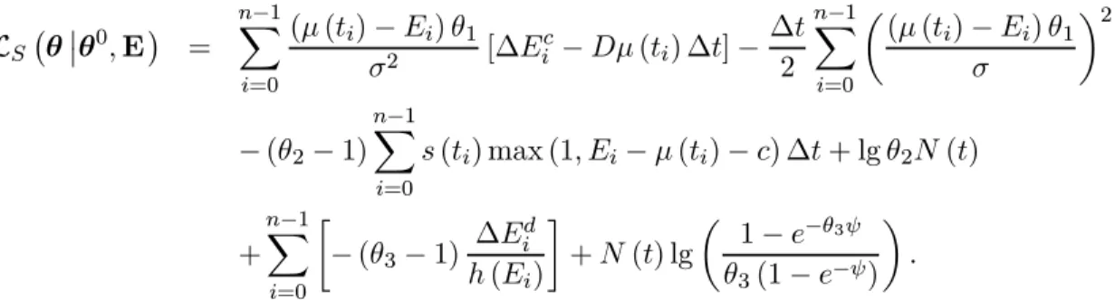
We compute the log-likelihood function L for the law of the diffusion process corresponding to an arbitrary parameter vector θ with respect to the law of the process under a prior reference parameter θ0. Its exact analytical expression is derived
in Appendix A. We decide to choose as starting parameter values θ1 = 0, θ2 = 1,
θ3 = 1 which correspond to an absence of drift, a normalized jump intensity and a
jump amplitude drawn from a truncated exponential distribution with parameter 1. The approximate logarithmic likelihood function reads as:
LD ¡ θ¯¯θ0, E¢ = n−1 X i=0 (µ (ti) − Ei) θ1 σ2 [∆E c i − Dµ (ti) ∆t] − ∆t 2 n−1 X i=0 µ (µ (ti) − Ei) θ1 σ ¶2 − (θ2− 1) n−1X i=0 s (ti) ∆t + lg θ2N (t) + n−1X i=0 · − (θ3− 1) ∆Edi h (Ei) ¸ + N (t) lg µ 1 − e−θ3ψ θ3(1 − e−ψ) ¶ ,
where Dµ (ti) denotes the first order derivative of µ at time ti. The first part is a
discretized version of the Doléan-Dade exponential for continuous processes. The re-maining terms come from the jump part of the process. The log-likelihood function explicitly depends on θ1, θ2, θ3, and on the filtered data set
¡
∆Ed, Ec¢, which in turn is derived from the original market data set E and the choice of parameter Γ. We maximize this function with respect to θ over a bounded parameter set Θ identified through economic interpretation of the model parameters. One may alternatively use Monte Carlo simulated samples to infer a reasonable parameter domain and starting values for the numerical optimization algorithm. We finally obtain a non-linear maxi-mization program of a continuous function over a compact set and classical theorems ensure the existence of a local maximum, which will be our estimate for θ∗.
can be obtained as: σ = v u u tn−1X i=0 ∆E (ti)2, (9)
where each summand ∆E (ti)2represents the square of the continuous part ∆Ec(ti) of
observed price variations (in a logarithmic scale) between consecutive days tiand ti+1,
net of the mean reversion effect |θ1× (µ (ti) − E (ti))|.5 This estimator converges to
the exact local covariance estimator for diffusion processes under continuous time ob-servations (Genon-Catalot and Jacod (1993)). We note that numerical experiments not reported here suggest that a time-dependent volatility does not produce a sig-nificant improvement in the estimated process (given the other specifications of our model); moreover in this case a joint estimation of volatility and mean reversion parameters would become necessary.
C. Alternative model specifications
We now consider two models displaying in their discontinuous component features either proposed in existing papers on electricity or that may be envisioned as im-provements of some kind.
First, by setting to +1 the jump direction function h defined in formula (4), we obtain a restricted model where upcoming jumps are all upward directed and reversion to normal levels is exclusively carried over by the smooth drift component. This upward-jump model represents the classical jump-diffusion extension of the continuous
diffusion models proposed over the years by Pilipovich (1997), Barlow (2002), Lucia and Schwartz (2002). All the remaining model specifications are the same as those of our signed-jump model. As a consequence, calibration to market data follows the steps described above, with one major exception: price variations of negative size all enter the estimation of the continuous part of the process (i.e., ∆Ed only contains positive jumps).
Alternatively, we may allow the jump intensity function ι defined in formula (2) to be stochastic. In order to account for the dependence of the likelihood of jump occur-rence on the price level following upward shocks, we consider the following function of the spot price and time:
ι¡t, E¡t−¢¢= θ2× s (t) ×
£
1 + max¡0, E¡t−¢− E (t)¢¤.
As in the case of the threshold T (t) defining the sign of the jump, we define E (t) as a constant c over the mean trend µ. If the spot price is below the mean trend µ plus this spread c, then intensity is purely time dependent. Each price-unit beyond this boundary amplifies accordingly the time dependent intensity. We identified that the best intensity function was provided by a choice of c equal to ∆/2 (i.e., an increasing jump occurrence when prices are above the median line between the mean trend µ (t) and the threshold T (t)). The ”max” function ensures that the jump intensity never goes below the ”standard level” θ2× s (t) (that may be viewed as the effect of random
intensity is displayed as a function of time and log-price.
Figure 8 about here
In this signed-jump model, jump occurrence is both time and level dependent.
Be-cause all the other model specifications are the same as those in the signed-jump model with deterministic intensity, calibration to market data follows the same steps as described above. The log-likelihood estimator denoted in this case as LR, becomes
slightly more complex:
LS ¡ θ¯¯θ0, E¢ = n−1 X i=0 (µ (ti) − Ei) θ1 σ2 [∆E c i − Dµ (ti) ∆t] − ∆t 2 n−1 X i=0 µ (µ (ti) − Ei) θ1 σ ¶2 − (θ2− 1) n−1 X i=0 s (ti) max (1, Ei− µ (ti) − c) ∆t + lg θ2N (t) + n−1 X i=0 · − (θ3− 1) ∆Ed i h (Ei) ¸ + N (t) lg µ 1 − e−θ3ψ θ3(1 − e−ψ) ¶ .
This expression shows that parameters θ1 and θ3 are unaffected by a change in the
jump intensity function as the corresponding term can be factored out of the likelihood estimator in absolute scale exp (LS).
VI. Empirical Results
The calibration procedure has been implemented on the U.S. data set described in section IV. We first present results for the signed-jump model, then discuss the quality of our assessments on the data set under analysis and finally conclude on a comparison with the alternative models introduced at the end of Section V.
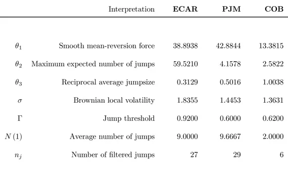
As mentioned before, the first step is the functional estimation of the structural elements µ, s, T , and p. The values α, β, γ, δ, ε, and ζ characterizing the average trend function µ (t) defined in formula (5) are reported in Table I.
Table I about here
The jump intensity shape s (t) is of the form defined in equation (6), with k = 1, τ = 0.5, and d = 2; this corresponds to a jump occurrence displaying an annual peak strongly clustered around the middle of the year, as observed in all examined markets. The threshold T (t) is defined by a spread ∆ over the deterministic trend µ(t), where ∆ in chosen in the order of 50 percent of the range spanned by the observed log-prices. We observe that both ECAR and PJM reveal no significant linear trend over the three-year sample period, while COB shows a small positive linear trend expressed by the coefficient β.
In all cases, the annual periodicity expressed by the coefficient γ prevails over the semiannual component described by the coefficient δ. Figure 9 represents the average
paths for the three regional markets in a joint graph; clearly, the annual component is predominant in the COB market, whereas an additional semiannual component is significant in the ECAR and PJM markets.
Figure 9 about here
A clear difference between the three markets is represented by the maximum size ψ of daily price variations: for instance, ECAR displays jumps which may be more than three times greater than the maximum value observed in the COB market. In this market, the high percentage of hydrogeneration and the reservoir capacity allow to go through the year - the cold season in particular - with no or mild spikes. In contrast, the PJM and ECAR markets experience both very warm summers and cold winters; this leads to the semiannual periodicity of observed power prices in these regions. However, PJM benefits from a fuel mix in power generation and also from a rich transmission network which has been very efficient since the start of deregulation; hence the less dramatic price spikes observed.
The second step of the calibration procedure is the statistical estimation of pa-rameters θ1, θ2, θ3, σ, Γ, and d. The approximated likelihood estimation detailed in
the previous section has been implemented by the Levenberg-Marquardt non-linear maximum search algorithm. Final results are reported in Table II.
All markets exhibit some amount of smooth mean reversion. Note that the value of the reversion force in PJM is significantly greater than ECAR. It is worth emphasizing again that the overall reversion displayed by our model is created by the joint effect of the classical mean reversion and an effect due to the downward jumps. Since ECAR displays more jumps than PJM, the overall reversion effect is higher than the one observed in the PJM market. This is statistically consistent with the fact that, in PJM, both skewness and kurtosis of daily price increments are lower since the smooth reversion suffices most of the time to ensure return to the average trend. We remark that the expected number of jumps per year is represented by the integral of the calibrated intensity function over one year.
We now turn to the assessment of the quality of the estimated processes. This is performed according to four criteria:
• First, we analyze simulated sample paths together with empirically observed trajectories and make a judgement about the fitting quality of the trajectorial properties.
• Second, we compare simulated moments of the daily increments distribution with the empirical values displayed by each market under investigation.
• Third, we check for the robustness of the procedure by re-estimating simulated sample paths generated by the calibrated model.
• Fourth, we test our model against the most popular representation of electricity spot prices so far, namely a jump-diffusion process with positive jumps only and smooth mean-reversion.
• Fifth, we examine the effect of introducing a price-dependent jump intensity on both trajectorial and statistical properties displayed by the most irregular market in our data set (ECAR).
Figures 10 to 12 show trajectories of the estimated model for the three markets.
Figures 10 to 12 about here
For the purpose of comparison, both historical and sample paths are reported at var-ious scales. The dashed line represents the average mean trend µ (t). These pictures show that the proposed family of processes is capable to reproduce quite consistently the qualitative features exhibited by power paths in all three examined markets.
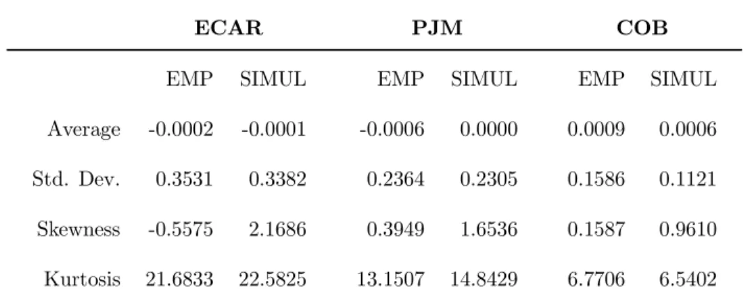
Table III reports the mean, standard deviation, skewness and excess of kurtosis of observed and simulated daily price variations.
Table III about here
We see that all statistics of the simulated trajectories are quite satisfactory; there is however a small positive skewness which has no counterpart in the empirical data, suggesting that the reverting component ought to be more pronounced. The most
important effect of the signed-jump model is the excellent fit of the leptokurtosicity of the distribution. The relevance of the incorporation of jumps in equity return mod-elling has been analyzed and exhibited in a number of recent papers of the financial economics literature (see for instance Carr, Geman, Madan, and Yor (2002)). In the case of electricity prices, the non-normality of distributions is widely recognized and kurtosis naturally becomes a key parameter: in these markets where extreme events provide the rational for building small and flexible power plants called peakers, a proper representation of the spikes and their probability of occurrence (i.e., of the tail of the distribution) is the first requirement a model must satisfy.
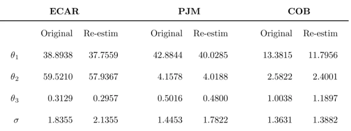
We further test the robustness of the estimators by simulating one thousand paths from the estimated process and then using the corresponding increments to reassess the values of the parameters θ1, θ2, θ3 and σ. The simulation method is detailed in
Appendix B and results are described in Table IV.
Table IV about here
For all estimated models the procedure is satisfactorily stable. We do not report the values for Γ because they are all identical to the original ones. The only slight mismatch occurs for the jump size parameter θ3 in the case of COB market; this
may be due to the very low number of jumps, which makes the estimator sensitive to outliers in the simulated paths. This result is of minor importance, to the extent that the jump component is almost irrelevant for the modelling of COB prices. In general,
we conclude that the procedure is not only statistically but also numerically robust. Returning to the alternative specifications discussed in Section IV.C, we also cal-ibrated the upward-jump model with deterministic intensity and the signed-jump model with stochastic intensity to the ECAR market data. For the purpose of com-parison, Table V shows the quality assessment of these two models with respect to the benchmark defined by the signed-jump model with a deterministic intensity.
Table V about here
It is clear that all three models account quite well for the first two moments of daily average prices, with an excess in volatility and positive skewness, however, for the upward-jump model. The signed-jump model with stochastic intensity compared to the one with deterministic intensity slightly improves the value of the skewness, and our view is that this extra-complexity does not bring any decisive improvement. As for the upward-jump model (with deterministic intensity) which is quite popular in the literature on electricity spot price modelling, it generates a kurtosis four times smaller than the real one; this mispecification may translate into a wrong estimation of Value at Risk numbers and have severe consequences in markets where some inefficient plants continue to exist only because of these rare events. In all industries a wrong estimation of reserves leads to harmful consequences.
VII. Conclusion
We have proposed in this paper a family of discontinuous processes featuring up-ward and downup-ward jumps to model electricity spot prices. Our approach is rooted in the physical properties of electricity, in particular its non-storability, and their consequences on the short-term supply and demand equilibrium in the pool market.
Given the number of state variables that explain power prices in a pool (i.e., temperature, fuel mix, type of transmission network) and their distributional com-plexity (e.g., plant outages occurrence), we chose a reduced-form representation in order to get a tractable and efficient tool allowing to handle the random evolution of spot prices and the related management decisions. The calibrated processes exhibit the expected mean reversion property, however in an unevenly pronounced manner depending on the market. All analyzed trajectories show price spikes resulting from momentary imbalance between offered generation and volume of demand. The fitting performed on three major U.S. markets allows to conclude positively on the quality of the model, both in terms of its statistical and trajectorial properties.
References
Andersen, Torben G., Luca Benzoni, and Jesper Lund, 2002, An Empirical Investigation of ContinuousTime Equity Return Models, Journal of Finance 57, 1239 -1284.
Ball, Clifford A. and Walter N. Torous, 1983, A simplified jump process for common stock returns, Journal of Financial and Quantitative Analysis 18, 53-65.
Bandi, Federico, 2000, On the functional estimation of jump-diffusion models, Work-ing Paper, University of Chicago.
Barlow, M.T., 2002, A diffusion model for electricity prices, Mathematical Finance 12(4), 287-298.
Barone-Adesi, Giovanni, and Andrea Gigli, 2002, Electricity Derivatives, Working Paper, National Center of Competence in Research, Università della Svizzera Italiana.
Beckers, Stan, 1981, A note on estimating the parameters of the jump-diffusion model of stock returns, Journal of Financial and Quantitative Analysis 16, 127-140.
Bessembinder, Hendrik, and Michael L. Lemmon, 2002, Equilibrium pricing and opti-mal hedging in equilibrium electricity forward markets, Journal of Finance 57, 1347-1382.
Bhanot, Karan, 2000, Behavior of power prices: implications for the valuation and hedging of financial contracts, Journal of Risk 2, 43-62.
Carr, Peter, Hélyette Geman, Dilip Madan, and Marc Yor, 2002, The fine structure of asset returns: an empirical investigation, Journal of Business 75, no.2, 305-333.
Deng, Shijie, 1999, Stochastic models of energy commodity prices and their applica-tions: mean reversion with jumps and spikes, Working Paper, Georgia Institute of Technology.
Escribano, Álvaro, Juan Ignacio Peña, and Pablo Villaplana, 2002, Modeling elec-tricity prices: international evidence, Working Paper, Departamento de Economia, Universidad Carlos III de Madrid.
Eydeland, Alexander, and Hélyette Geman, 1998, Pricing power derivatives, Risk (October).
Eydeland, Alexander, and Krzysztof Wolyniec, 2002, Energy and Power Risk man-agement: new developments in modeling, pricing and hedging (Wiley, Chicago).
Fama, Eugene, and Kenneth French, 1987, Commodity futures prices: Some evidence on forecast power, premiums and the theory of storage, Journal of Business 60, no.1, 55-73.
Geman, Hélyette, and Oldrich Vasicek, 2001, Forwards and futures contracts on non-storable commodities: the case of electricity, Risk ( August).
Genon-Catalot, Valentine, and Jean Jacod, 1993, On the estimation of the diffu-sion coefficient for multidimendiffu-sional diffudiffu-sion processes, Annales de Institut Henri Poincaré 29, no.1, 119-151.
Gihman, Iosif Il’Ich, and Anatoli V. Skorohod, 1972, Stochastic Differential Equations (Springer, NewYork).
Huisman, Ronald, and Ronald Mahieu, 2001, Regime jumps in electricity prices, Working Paper, Rotterdam School of Management, Erasmus University Rotterdam.
Jacod, Jean, and Albert Shiryaev, 1987, Limit Theorems for Stochastic Processes, (Springer, New York).
Johannes, Michael, 1999, Jumps in interest rates: a nonparametric approach, Working Paper, University of Chicago.
Kaldor, N,. 1939, Speculation and economic stability, Review of Economic Studies 7, 1-27.
Litzenberger, Robert H., and Nir Rabinowitz, 1995, Backwardation in oil futures markets: theory and empirical evidence, Journal of Finance 50, 1517-1545.
Lo, Andrew, 1988, Maximum likelihood estimation of generalized Ito processes with discretely sampled data, Econometric Theory 4, 231-247.
Lucia, Julio J., and Eduardo S. Schwartz, 2002, Electricity prices and power deriva-tives: evidence from the Nordic Power Exchange, Review of Derivatives Research 5, 5-50.
Pedersen, Asger Roer, 1995, A new approach to maximum likelihood estimation for stochastic differential equations based on discrete observations, Scandinavian Journal of Statistics 22, 55-71.
Pilipovich, Dragana, 1997, Energy Risk: Valuing and Managing Energy Derivatives (McGraw-Hill, New York).
Pindyck, Robert, 1999, The long-run evolution of energy commodity prices, Energy Journal, April, IAEE.
Pirrong, Craig, 2001, The price of power: the valuation of power and weather deriv-atives, Working Paper, Oklahoma State University.
Roncoroni, Andrea, 2002, Essays in Quantitative Finance: Modelling and Calibra-tion in Interest Rate and Electricity Markets, PhD DissertaCalibra-tion, University Paris Dauphine.
Routledge, Bryan R., Duane J. Seppi, and Chester S. Spatt, 2000, Equilibrium forward curves for commodities, Journal of Finance 55, 1297-1338.
Rubinstein, Reuven, 1981, Simulation and the Monte Carlo method, (John Wiley & Sons, London).
Working, Holbrook, 1949, The theory of the price of storage, American Economic Review 39, 1254-1262.
Yin, Y.Q., 1988, Detection of the number, locations and magnitude of jumps, Com-munications in Statistics: Stochastic Models 4, 445-455.
Footnotes
1. In most markets, this price for date t is defined the day before by the clearing of buy and sell orders placed in the pool.
2. Up to now, negative electricity prices have rarely been observed.
3. If t is a jump date, the continuous part of the path is assumed to be constant between t and the next sample date. Since spikes are rare and typical price variations are much smaller than those occurring during a spike, this simplification does not introduce any significant bias in the estimation procedure.
4. τ is called ”the phase” in the language of sinusoidal phenomena.
5. Note that in contrast to classical settings where the mean reversion feature was introduced (e.g., interest rates, stochastic volatility) the difference µ (t) − E (t) may be quite large in the case of electricity prices. This observation was made in Section III of the paper.
List of Figures
Figure 1. The power stack function for the ECAR Market.
The generation cost is mildly increasing until a load threshold is reached; then the supply curve exhibits strong convexity.
Figure 2. Empirical Price Returns Distributions vs. Normal Distributions with Equal Means and Variances.
For each market, the empirical density of price returns is reported together with a normal density matching the first two moments. All markets display strong deviations from normality due to the presence of upward and downward jumps.
Figure 3. ECAR Price Path (January 6, 1997 - December 30, 1999). Spikes concentrate in summer, where prices may rise as high as 2000 U.S. dollars per kilowatt-hour.
Figure 4. PJM Price Path (January 6, 1997 - December 30, 1999).
Spikes concentrate in summer, where prices move up to a level of 400 U.S. dollars per kilowatt-hour.
Figure 5. COB Price Path (January 6, 1997 - December 30, 1999).
Spikes concentrate in summer, where prices rise to values around 100 U.S. dollars per kilowatt-hour.
Figure 6. Time-Dependent Jump Intensity Function.
The time-dependent jump intensity function is designed to concentrated jump occur-rence during the warm season. Parameter d drives the degree of cluster.
Figure 7. Sample Jumps of a Time-Dependent Jump Intensity Function. The time-dependent jump intensity function is designed to concentrated jump occur-rence during the warm season. Dotted tags signal the sample jump times of a Poisson process corresponding to the displayed time-dependent intensity function.
Figure 8. Stochastic Jump Intensity Function.
Jump intensity depends on time and electricity price level. If the spot price is below the mean trend µ plus the spread ∆/2, then intensity is only time dependent. Each price-unit beyond this boundary amplifies accordingly the time dependent intensity.
Figure 9. Estimated Average Trends in the Observed Log-Price Paths (January 6, 1997 - December 30, 1999).
PJM and ECAR markets exhibit overlapping periodicities with periods equal to 6 and 12 months. COB essentially displays an annual periodicity.
Figure 10. ECAR Simulated Price Path vs. Empirical Path. Panel (a): absolute scale 0-2500. Panel (b): absolute scale 0-500. Panel (c): absolute scale 0-100.
Figure 11. PJM Simulated Price Path vs. Empirical Path. Panel (a): absolute scale 0-600. Panel (b): absolute scale 0-300. Panel (c): absolute scale 0-100
Figure 12. COB Simulated Price Path vs. Empirical Path. Panel (a): absolute scale 0-175. Panel (b): absolute scale 0-90. Panel (c): absolute scale 0-50.
Appendix A. Likelihood Estimator
The following proposition is an important result for the estimation of jump processes, both from a theoretical and operational standpoints, and an original contribution of the paper (to our knowledge, at least).
Proposition. Let µ, s, f, c and σ be sufficiently regular functions for the stochastic differential equation (1)-(4) to admit a unique weak solution Eθ for all θ = (θ1, θ2, θ3)
in a compact subset of R3+. Let E = {E (t) , t0 ≤ t ≤ t} be an observed path over the
continuous time interval [t0, t] and θ0 =
¡
θ01, θ02, θ03¢ a starting parameter set. Then the log-likelihood of observing a realization of the process Eθ with respect to the process Eθ0 is given by: L¡θ¯¯θ0, E¢ = Z t t0 [µ (u) − E (u−)]¡θ1− θ01 ¢ σ (u)2 d £ Ec¡u−¢− µ (u)¤ (10) −12 Z t t0 µ [µ (u) − E (u−)] θ1 σ (u) ¶2 du − µ θ2 θ02 − 1 ¶ Z t t0 s (u) du +¡lg θ2− lg θ02 ¢ N (t) + X u≤t,∆E6=0 ·¡ θ3− θ03 ¢ f µ ∆E (u) h (E (u−)) ¶ − lg c (θ3) + lg c ¡ θ03¢ ¸ ,
where Ec is the path process devoid of its jump component:
Ec¡u−¢= E¡u−¢− E0−
X
s≤u,∆E(s)6=0
∆E (s) , (11)
E0 is the starting point E (t0), ∆E (s) is the observed jump size at time s (if any),
Proof.
For notational simplicity, we write equation (1) as:
dE = (α + θ1β) dt + σdW + hdJ (12)
with α = Dµ (t), β = µ (t) − E (t−), h = h (E (t−)) and set t0 = 0. We also denote
E (t−) by E−.
We divide the proof in two steps. First, we compute the semimartingale charac-teristic triplet (Bθ, C, νθ) of the jump-diffusion process E corresponding to a given
choice of the parameter θ. Second, we calculate the likelihood by applying a general semimartingale version of the Girsanov theorem (see Jacod and Shiryaev (1987)). Step I - Since N is independent of Ji for all i, Eθ(N (t)) = ι (t), Jii.i.d.∼ p (x; θ3), and
the additive compensator of the purely discontinuous part of the semimartingale E is given by: νθ(dt × A, t) = νθ(A, t) dt = Eθ h¡E−¢dt N (t)X i=1 Ji dt = " θ2s (t) Z [0,ψ] dx¡1A\{0}¡h¡E−¢x¢p (x; θ3) ¢# dt = · θ2s (t) Z X x h (E−)p µ x h (E−); θ3 ¶¸ dxdt. where X = ³h 0,h(Eψ−) i ∩ A ´
\ {0}. Since all coefficients are bounded functions, the process E is a special semimartingale. Consequently, the canonical representation
of equation (12) follows by adding and subtracting the compensator νθ to the jump
measure dµθ = h(t) dJ(t) and gathering the absolutely continuous terms:
dE = Ã α + βθ1+ Z [0,ψ] dνθ(x, t) ! dt + σdW + dµθ,
where µθ is a martingale measure under Pθ. From this expression we immediately
identify the term of the semimartingale triplet corresponding to θ:
Bθ(t) = Z t 0 " α (u) + β (u) θ1+ Z [0,ψ] h¡E−¢xdνθ(x, u) # du, (13)
Step II - The semimartingale process under the prior probability Pθ0 is determined by the characteristic triplet (Bθ0, C, νθ0). Since:
νθ(dt × A) = dt Z X dx ½ θ2 θ02 exp ·¡ θ3− θ03 ¢ f µ x h (E−) ¶ −¡lg c (θ3) − lg c¡θ03 ¢¢¸ ×θ02s (t) x h (E−)exp · θ03f µ x h (E−) ¶ − lg c¡θ03¢ ¸¾ = Z X θ2 θ02 exp ·¡ θ3− θ03 ¢ f µ x h (E−) ¶ − lg c (θ3) + lg c ¡ θ03¢ ¸ νθ0(dt × dx) ,
the density of dνθ with respect to dνθ0 is given by:
dθ(t, x) = θ2 θ02exp ½¡ θ3− θ03 ¢ f µ x h (E−) ¶ − lg c (θ3) + lg c ¡ θ03¢ ¾ .
By substituting this expression into (13), we see that the drift term under Pθ can be
represented as the sum of the drift term under Pθ0 and a term denoted as cθ(t) σ (t),
where: cθ(t) = β (t) £ θ1− θ01 ¤ σ (t)−1.
Let Pθ|Ft be the probability measure induced by Eθ over the path space and
re-stricted to events up to time t. Given the set E of continuous time observations, the corresponding density of Pθ|Ft with respect to the prior probability Pθ0|Ft is given
by the Radon-Nikodym derivative: dPθ dPθ0 ¯ ¯ ¯ ¯ Ft = exp ½Z t 0 · cθdW − 1 2c 2 θdu − Z X ((dθ− 1) dνθ0+ lg dθdµ) ¸¾ .
This is a consequence of the Girsanov theorem on measure changes for general semi-martingales (see Jacod and Shiryaev (1988)). The first two factors can be written as: exp ½Z t 0 · cθdW − 1 2c 2 θdu ¸¾ = exp (Z t 0 β¡θ1− θ01 ¢ σ2 d · E (u) − Z u 0 α (v) dv − X s≤u,∆E(s)6=0 ∆E (s) − 12Z t 0 β2¡θ1− θ01 ¢2 σ2 du . The third factor is:
exp ½ − ZZ (dθ− 1) dνθ0 ¾ = exp ½ − Z t 0 s (u) · θ2 θ02 Z X p µ x h (E−); θ3 ¶ dx − Z X p µ x h (E−); θ 0 3 ¶ dx ¸ du ¾ = exp ½ − µ θ2 θ02 − 1 ¶ Z t 0 s (u) du ¾ ,
The fourth factor is: exp ½Z t 0 Z X lg dθdµ ¾ = exp ½Z t 0 Z X ·¡ θ3− θ03 ¢ f µ x h (E−) ¶ − lg c (θ3) + lg c ¡ θ03¢ ¸ dµ +¡lg θ2− lg θ02 ¢ Z t 0 Z X dµ ¾ = exp X u≤t,∆E(u)6=0 ·¡ θ3− θ03 ¢ f µ ∆E (u) h (E−) ¶ − lg c (θ3) + lg c ¡ θ03¢ ¸ +¡lg θ2− lg θ02 ¢ N (t) ,
where the last equality stems from the relation between the process and the measure representation of any marked point process. Substituting the expressions of α and β leads to the log-likelihood function (10). Q.E.D.
Appendix B. Simulation Algorithm
Monte Carlo simulations of trajectories described in equation (1) serve three purposes. First, they provide a starting value θ0 for the maximum likelihood search algorithm. This is accomplished by sampling trajectories for several parameter sets until we find one whose corresponding simulated paths show qualitative features comparable with those displayed in the empirical observations. Second, sample trajectories allow one to judge upon the qualitative performance of the calibrated model and to compute simulated moments of various orders for the daily price variations. This is used for moment matching in the last step of the calibration procedure. Third, simulations provide a robustness analysis of the estimation procedure: parameters of a calibrated model can be re-estimated over simulated paths. The closer to the original values are the re-estimated ones, the more robust the likelihood estimation procedure is. We detail a simulation algorithm for sampling a path defined by equation (1). The Euler approximation of the stochastic differential equation (1) over a discrete set of evenly-spaced sample times t1, ..., tN is:
Ek+1= Ek+ Dµ (tk) × ∆ + θ1[µ (tk) − Ek] × ∆ + σ
√
∆N + h (tk) × 1i× J,
where N is a sample from a standard normal distribution and J is a sample from p (·, θ3). The function 1i is either 1 or 0 according to whether ti is, or is not, a jump
con-stant deterministic intensity, we may first simulate jump times of a concon-stant intensity Poisson process and then use a variation of the ”acceptance-rejection” method to make sure that these are statistically identical to the required sample set of times. More precisely, on a given horizon [0, T ], we generate inter-arrival times εi until their
sum exceeds T . Each εi is a sample from an exponential distribution with parameter
ι∗ = maxt∈[0,T ]ι (t). Candidate jump times τ0k are defined by approximating each Pk
i=1εi to the closest element in the set of sample times {t1, ..., tN}. For each k,
we draw a uniform random variable Uk on [0, ι∗] and accept τ0k if Uk ≤ ι (τ0k),
oth-erwise reject it. The set of selected times is hence a sample sequence (τ1, ..., τn) of
the jump times for a compound jump process with intensity function ι (t). Conse-quently, 1i= 1 if ti= τk, for some k = 1, ..., n. This completes the description of the
Table I
Estimated ”Structural” Elements The electricity log-price model:
dE (t) = Dµ (t) dt + θ1
£
µ (t) − E¡t−¢¤dt + σdW (t) + h¡t−¢dJ (t) , with average trend function:
µ (t; α, β, γ, δ, ε, ζ) = α + βt + γ cos [ε + 2πt] + δ cos [ζ + 4πt] , and jump component:
h¡t−¢ = 1, if E¡t−¢< µ (t) + ∆; − 1 otherwise, (Direction) J (t) = XN (t) i=1 Ji, with Ji i.i.d. ∼ p (x; θ3, ψ) ∝ eθ3f (x), 0 ≤ x ≤ ψ, (Size) ι (t) = θ2× (2/ (1 + |sin [π (t − τ) /k]|) − 1)2, (Intensity)
is calibrated to a data set including daily observations between January 6, 1997 and December 30, 1999. Observed log-prices over the three-year period are averaged into a one-year period and bounded from above by the 0.7-quantile ν of their empirical distribution. The trend function µ is fitted to the average data by a sequential OLS providing parameters α, β, γ, δ, ε, and ζ. The regime-switching threshold T is set as a spread ∆ over the average trend µ. The jump-size distribution takes values in the interval [0, ψ], where ψ is chosen as the observed maximal daily absolute variation in log-prices. The shape of the jump intensity is described through the parameters k and τ .
Interpretation ECAR PJM COB
α average log-price level 3.0923 3.2002 2.8928 β average log-price slope 0.0049 0.0036 0.1382 γ yearly trend -0.1300 0.0952 0.1979 δ 6-month trend 0.0292 0.0217 0.0618 ε yearly shift 0.3325 2.4383 1.7303 ζ 6-month shift 0.7417 0.2907 1.7926 ν 0.7 avg distr. quantile 3.2762 3.3232 3.3586 ∆ jump regime level 2.5000 1.5000 1.0000 ψ maximum jump size 3.3835 1.6864 1.0169 k jump periodicity 1.0000 1.0000 1.0000 τ intensity phase 0.5000 0.5000 0.5000