Model order reduction applied to the numerical study of electrical motor based on POD method taking into account rotation movement

(1)

is an open access repository that collects the work of Arts et Métiers Institute of Technology researchers and makes it freely available over the web where possible.

This is an author-deposited version published in: https://sam.ensam.eu Handle ID: .http://hdl.handle.net/10985/9559

To cite this version :

Thomas HENNERON, Stéphane CLENET - Model order reduction applied to the numerical study of electrical motor based on POD method taking into account rotation movement

-INTERNATIONAL JOURNAL OF NUMERICAL MODELLING: ELECTRONIC NETWORKS, DEVICES AND FIELDS - Vol. 27, n°3, p.485-494 - 2014

(2)

INTERNATIONAL JOURNAL OF NUMERICAL MODELLING: ELECTRONIC NETWORKS, DEVICES AND FIELDS Int. J. Numer. Model. 2010; 00:1–10

Published online in Wiley InterScience (www.interscience.wiley.com). DOI: 10.1002/jnm

Model order reduction applied to the numerical study of electrical

motor based on POD method taking into account rotation

movement

T. Henneron

1∗

and S. Cl´enet

2

1_{L2EP/Université Lille1, Cité Scientifique, 59655 Villeneuve d’Ascq, France.} 2_{L2EP, Arts et Métiers ParisTech, 59046 Lille, France}

SUMMARY

In order to reduce the computation time and the memory resources required to solve an electromagnetic field problem, Model Order Reduction (MOR) approaches can be applied to reduce the size of the linear equation system obtained after discretisation. In the literature, the Proper Orthogonal Decomposition (POD) is widely used in engineering. In this paper, we propose to apply the POD in the case of a Finite Element problem accounting for the movement. The efficiency of this method is evaluated by considering an electrical motor and by comparing with the full model in terms of computational time and accuracy.

Copyright c⃝2010 John Wiley & Sons, Ltd. Received . . .

KEY WORDS: proper orthogonal decomposition, finite element method, electrical motor

1. INTRODUCTION

Applying numerical method such as the Finite Element Method to solve model based on partial derivative equation can lead to huge linear equation system to solve. In order to reduce the computation time required to solve this equation system, Model Order Reduction (MOR) approaches can be applied to reduce the size of the system. In the literature, the Proper Orthogonal Decomposition (POD) is widely used in engineering, as for example to study turbulent fluid flows or structural vibrations. This approach has been introduced by [1] in turbulence in order to extract the most energetic structures of the flow. In term of practical aspect, the method of snapshots introduced by [2] enables to reduce the computational requirements of the POD calculations. The POD approach has been already applied in computational electromagnetics to solve linear or non linear magnetoquasistatics and electroquasistatics problems [3][4][5][6][7]. The accounting of movement was not addressed until now whereas it is an important feature when studying rotating electrical machine. In this paper, we propose to apply the POD approach with a numerical model obtained from the Finite Element method. Magnetostatics problem express in term of potential formulations is considered. A electrical motor is studied with POD models and then to take into account the rotation movement with reduced models.

In a first part, the numerical models obtained from the scalar and vector potential formulations are presented. In the second part, the proper orthogonal decomposition approach is developed in the case of a rotation movement. Finally, The reduced models are applied to study a synchronous ∗_{Correspondence to: thomas.henneron@univ-lille1.fr}

†_{Please ensure that you use the most up to date class file, available from the JNM Home Page at}

http://www3.interscience.wiley.com/journal/4673/home

Copyright c_⃝2010 John Wiley & Sons, Ltd.

(3)

machine with the scalar and vector potential formulations. Two methods derived from the POD to choose the number of snapshots on the period of rotation have been compared.

2. NUMERICAL MODEL 2.1. Magnetostatic problem

Let us consider a domainDof boundaryΓ(Γ = ΓB∪ ΓHandΓB∩ ΓH = 0). InD, the source of

magnetic field is created by permanent magnets and stranded inductors. We assume that the domain

D is divided into two parts: the static part and the moving part. The position of the moving part is given by an angleθ with respect to the static part (Fig.1). In the following, we will consider only the movement of rotation but the method can be also applied with a movement of translation or a combination of translation and rotation. Even though the approach remains valid with several stranded inductors and permanent magnets, we consider only one stranded inductor in the static part and one permanent magnet in the moving part.

Figure 1. Computational domain

The magnetostatic field problem can be described by using Maxwell’s equations,

curl H(x, θ) = Js(x) (1)

div B(x, θ) = 0 (2)

with H the magnetic field,Jsthe known current density flowing through the stranded inductors

andBthe magnetic flux density. Taking into account the material behavior, the constitutive relation between the fieldsBandHmust be considered. In the linear case, we have

B(x, θ) = µH(x, θ) + Br(x, θ) (3)

with µ the magnetic permeability and Br the remanent magnet flux density of the permanent

magnet. To get a unique solution, the following boundary conditions must be prescribed,

H(x, θ)× n = 0 on ΓH (4) B(x, θ)· n = 0 on ΓB (5)

withnthe outward unit normal vector. 2.2. Potential formulations

To solve the previous problem, two potential formulations can be used: the vector and scalar potential formulations.

(4)

MOR APPLIED TO THE NUMERICAL STUDY OF ELECTRICAL MOTOR BASED ON POD METHOD 3

2.2.1. Vector potential formulation

A magnetic vector potentialAis defined in the whole domain according to (2) such that:

B(x, θ) = curl A(x, θ) with A(x, θ)× n = 0 on ΓB (6)

Combining the previous expression and the behavior law, we obtain the vector potential formulation of the problem to be solved. The weak form is then written

∫

D 1

µcurl A(x, θ)· curl A

′_{(x, θ)dD =} ₍₇₎ ∫ D 1 µBr(x, θ)· curl A ′_{(x, θ)dD +}∫ D Js(x)· A′(x)dD

whereA′(x, θ)is a test function defined on the same space ofA(x, θ). In the 3D case, the vector potential is semi-discretised in the edge shape function space [8]

A(x, θ) = Ne

∑

i=1

Ai(θ)wai(x, θ) (8)

with Ai(θ) the circulation of the vector potentialA(x, θ)along the i-th edge, Ne the number of

edges of the mesh andwaithe edge shape function associated with the i-th edge. The circulation of waialong the i-th edge is equal to one and zero on all others edges [8][9]. In the stator, the shape

functions does not depend onθ. Only shape functions related to the rotor are angle dependent. We denote byAD(θ)the vector of components(Ai(θ))1≤i≤Ne. The vectorJsis expanded in the facet

shape function space. This field can be determined by a tree technic to impose its free divergence [10][11]. Then, we solve the following equations system

MA(θ)AD(θ) = FA(θ) (9)

withMA(θ)aNe× Nesquare matrix which the entriesmA(θ)i,jsatisfy

mA(θ)i,j=

∫

D 1

µcurl wai(x, θ)· curl waj(x, θ)dD

andFA(θ)aNe× 1vector with

fA(θ)i= ∫ D 1 µBr(x, θ)· curl wai(x, θ)dD + ∫ D Js(x)· wai(x)dD

2.2.2. Scalar potential formulation

A scalar potentialΩis defined in the whole domain according to (1) such that

H(x, θ) = Hs(x)− grad Ω(x, θ) with curl Hs(x) = Js(x) (10) Ω(x, θ) = 0 on ΓH and Hs(x)× n = 0 on ΓH

Combining the previous relation and the behavior law, we obtain the scalar potential formulation of the problem. The weak form to be solved is then written

∫ D µgrad Ω (x, θ)· grad Ω′(x, θ)dD = (11) ∫ D Br(x, θ)· grad Ω′(x, θ)dD + ∫ D µHs(x)· grad Ω′(x)dD

Copyright c_⃝2010 John Wiley & Sons, Ltd. Int. J. Numer. Model. (2010)

(5)

withΩ′(x, θ)a test function defined on the same space ofΩ. In the 3D case, the scalar potential is semi-discretised in the node shape function space

Ω(x, θ) = Nn

∑

i=1

Ωi(θ)wni(x, θ) (12)

withwnithe node shape function associated with the i-th node,Ωi(θ)a function of the angleθand Nnthe number of nodes of the mesh. The value ofwniis equal to one on the i-th node and zero on

all others nodes. We denote byΩD(θ)the vector of components(Ωi(θ))1≤i≤Nn. The vectorHsis

expanded in the edge shape function space [8]. Then, we solve the following equations system

MΩ(θ)ΩD(θ) = FΩ(θ) (13)

withMΩ(θ)aNn× Nnsquare matrix which the entriesmΩ(θ)i,jsatisfy

mΩ(θ)i,j=

∫

D

µgrad wni(x, θ)· grad wnj(x, θ)dD (14)

andFΩ(θ)aNn× 1vector with

fΩ(θ)i = ∫ D Br(x, θ)· grad Ω′(x, θ)dD + ∫ D µHs(x)· wni(x)dD

2.2.3. Locked step method

To take into account the movement of the moving part with respect to the static part of the system, the locked step method can be used with the scalar and vector potential formulations. This method, mainly used to study electrical motors in the literature [12] [13], imposes constraints on the mesh of the boundary between the static part and the moving part which requires to be meshed with a regular grid. The rotation movement is simply modeled by a circular permutation of unknowns on the mesh of the common surface of the moving part. We denote by∆θthe angular step between two positions of the moving part. Then, the rotation angleθis discretised byθk = k∆θ. In the following,

we denote by

M (θ)XD(θ) = F (θ) (15)

the equation system (9) or (13).

3. PROPER ORTHOGONAL DECOMPOSITION

The Proper Orthogonal Decomposition is based on a separated representation of functions of the solution [1] [2]. In our case, if we denote byX(x, θ) the scalar or vector potential (see (8) and (12)), we can write X(x, θ)≈ M ∑ n=1 Rn(x)Sn(θ) (16)

withRn(x)defined onD,Sn(θ)defined on[θ0, θT]withθ0andθT the initial and final angles and M the number of modes taken into account for the approximation of the solution. The functions

Rn(x)form an orthogonal basis which verify

∫

D

(6)

whereδij is the knonecker product. The functionsSn(θ)can be expressed from the projection of X(x, θ)on the basis of functionsRn(x)such that

Sn(θ) =

∫

D

X(x, θ)· Rn(x)dD (18)

To determine the set of functionsRn(x), we aim at minimizing the quantity ∥X(x, θ) − M ∑ n=1 Rn(x)Sn(θ)∥2 (19) =∥X(x, θ) − ( M ∑ n=1 ∫ D X(x, θ)· Rn(x)dD)· Rn(x)∥2

with∥∥2the L2-norm. To determine a discrete representation of the functionsRn(x), the Snapshot

method can be used [2]. In a first step, the matrix system (14) is solved forM angular steps (called Snapshots). TheM vectors ofXD(θk)obtained at each angular step are gathered in a matrixMS.

Then, the matrixMSof sizeNx× M is defined withNxthe number of unknowns (nodes or edges

depending on the formulation) of the mesh. The discrete forms of (17) and (15) can be written as

Ψ = MSR (20)

MS = ΨMSr (21)

whereRis a matrix whose the columnicorresponds to the discrete values of the functionRi(x)(in

the edge or nodal element space),Ψthe discrete projection operator between the values ofXin the basis of theNxfunctions and the reduced basis. The expression ofΨcan be deduced from a Singular

Value Decomposition (SVD) of the matrix of SnapshotsMS. Then, we obtainMS = V ΣWtwith

Σthe diagonal matrix of the singular values,V andW the orthogonal matrices of the left and right singular vectors. By combining (19), (20) and the SVD ofMS, we have

MS = V ΣWtRMSr (22)

By assuming thatR = W, we haveW Wt= I. The previous equation can be simplified as:

MS = V ΣMSr (23)

By identification, the expression ofΨcan be defined such thatΨ = V Σ. The reduced matrix system can be deduced by using the operatorΨin (14)

Mr(θ)Xr(θ) = Fr(θ) (24)

with Mr(θ) = ΨtM (θ)Ψ and Fr(θ) = ΨtF (θ)

The size of the matrixMr and the vectorFr depend on the number of Snapshots. To obtain the

solution on[θ0, θT], the reduced matrix system is solved for all angular steps. As the matrixMr(θ)

depends on the angle, the matrix M (θ)is determinated at each angular step. For each step, the solution in the original basis can be determined such that

XD(θ) = ΨtXr(θ) = M

∑

n=1

ΨtiXrn (25)

In term of implementation, the computational cost of the singular value decomposition of MS

can be important due to the size of snapshot matrix. Another approach to obtain the expression of W can be carried out by the calculation of the eigenvalue decomposition of the correlation matrix defined byCM =

1 MM

t

sMs. The size ofCM isM× M and the SVD of this matrix give CM = W Σ2Wt.

(7)

4. APPLICATIONS

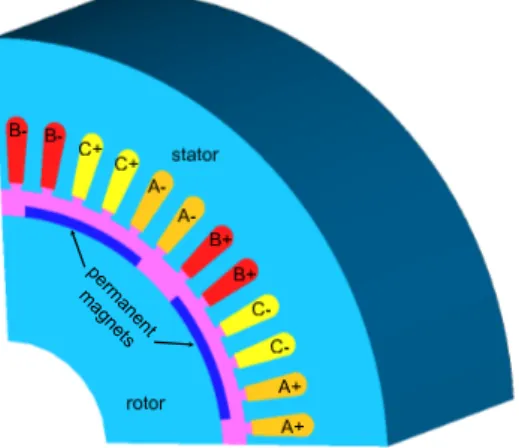
In term of applications, a permanent magnets synchronous machine is studied. This machine is composed of three phases and 8 poles. The rotation movement of the rotor is imposed at the angular speed100π rad/s. The three phases of the stator are not connected with an electrical circuit. We study the magnetic flux associated with a phase created by the permanent magnets of the rotor. Due to symetries, only one eighth of the machine is modelled (Fig. 2). The rotation of the rotor is taken into account with the locked step approach. The angular step between two successive positions of the rotor is ∆θ = π/80. The 3D spatial mesh has 40449 nodes and 53672 prisms. The electrical motor is studied with the full and reduced models from the potential formulations. For the scalar and vector formulations, the number of unknown is40311 and60377respectively. With the POD approach, two methods to choose the M snapshots on the period of rotation are compared. In the first approach, snpashots are the solutions of theMfirst positions of the rotor. The snapshots correspond to successive positions (∆θsp= ∆θ). In the second approach,M snapshots

are uniformly distributed on the whole interval [0, π/2] (∆θsp= π/2M). In the following, we

denote by ”reference model” the full model solved with the original mesh before reduction. We will compare in terms of computational time and accuracy the reduced model with the reference model.

Figure 2. Permanent magnets synchronous machine

4.1. Influence of the number of modes on the magnetic flux associated with a phase

Figures 3 and 4 present the magnetic flux of a phase obtained from the reference and POD models with the scalar and vector potential formulations by using the M first time steps as snapshots (∆θsp= ∆θ). On both figures, the curves of the magnetic flux computed with the POD models

diverge to the reference when the angle is greater thanM ∆θ. The solution of the reduced model on the position corresponding to the snapshot should give the same result as the full model. That is why the reference model and the reduced model give the same result for theM first positions. Figures 5 and 6 present the magnetic flux of a phase obtained from the reference and POD models with the scalar and vector potential formulations in the case of the snapshots uniformly distributed on [0, π/2] (∆θsp= π/2M). On both figures, the shape of curves converge until the ones of the

reference with respect to the number of snapshots. The error between the results obtained from a reference model and a POD approach can be expressed such thatε = ∥Φref − Φpod∥

2 ∥Φref∥2

withΦthe vector of discrete values of the magnetic flux. For the scalar formulation, 12 snapshots are required to obtain a good approximation of the solution with an error equal to0.009%and 15 snapshots for the vector potential formulation with an error equal to0.007%. In the case of an uniform distribution

(8)

of snapshots, the reduced basis are more accurate to approximate the solutions on[0, π/2]than by using theM first time steps.

Figure 3. Magnetic flux associated with a phase obtained from reference and POD models with the scalar formulation by using the M first time steps as snapshots

Figure 4. Magnetic flux associated with a phase obtained from reference and POD models with the vector formulation by using the M first time steps as snapshots

4.2. Influence of the number of modes on the distribution of the magnetic flux density

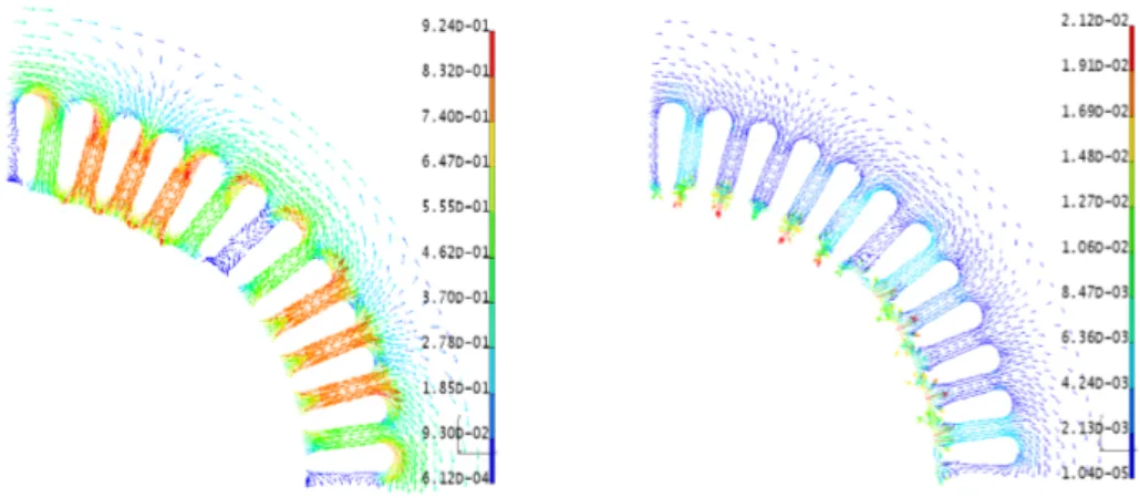
From equation (24) of the approximated solution, it is possible to represent a distribution of the magnetic flux density associated to each vector of the reduced basis. Figure 7 shows the distributions of Bi= curl ΨtiXri with i = 1, 2, 3 at a given angle θk obtained from the vector

potential formulation in a cross section of the stator. The distributions ofB2andB3are similar but

shifted with an electrical angle ofπ/2. It can be interpreted as a field distribution due to the rotor permanent magnets in the d-axis and q-axis. the fieldB1represents the distribution of the magnetic

flux density at the extremity of the teeth.

Figure 8 shows the distribution of the magnetic flux density obtained from the POD model of the vector potential formulation and the difference with the reference model at a given angle. A good approximation of the solution is obtained and we can note that the maximum of the error is not located where the magnetic flux density is the most important.

(9)

Figure 5. Magnetic flux associated with a phase obtained from reference and POD models with the scalar formulation by using an uniform distribution of the snapshots on[0, π/2]

Figure 6. Magnetic flux associated with a phase obtained from reference and POD models with the vector formulation by using an uniform distribution of the snapshots on[0, π/2]

Figure 7. Distribution ofB1,B2andB3(T)

4.3. Computational time

For 80steps corresponding to different positions of the rotor, the computation time is equal to9

minutes for the scalar formulation and 33 minutes for the vector formulation. In the case of 12

snapshots for the scalar formulation, the reduced model needs8minutes and for15snapshots with the vector formulation, the computation time is 10 minutes. These computation times take into

(10)

Figure 8. Distribution ofB(T) obtained from the reduced model of the vector formulation and its difference with the reference model

account the simulations of the reference models for the snaphots and those of the reduced models for 80angular steps. For one iteration, the ratio of computation time between the reference and reduced models is1.35and8.67for the scalar and vector formulations respectively. The small size of the reduced model explain the reduction of the computational time. The iterative method, in our case based on a conjugate gradient, requires less iterations with the reduced models than with the reference models. In our case and as usual, the solving of the reference models based on the scalar formulation is faster than the one of the vector potential formulation. However, with the two reduced models associated with both formulations, the unknown number and the computational times are similar.

5. CONCLUSION

The Proper Orthogonal Decomposition method associated with the 3D vector and scalar potential formulations has been developed in order to study electrical motors. The rotation of the rotor has been taken into account with the locked step approach. Two methods to choose the positions of snapshots computations on the period of rotation have been compared. With our application example, the use of an uniform distribution of the snapshots on the period of rotation gives better results compared with those obtained from the use of the first positions of the rotor. Then, it appears that the accuracy of the solution obtained from a reduced model is similar compared with this one of a fully described model. Finally, the computation time of the model order reduction approach remains lower than the one obtained with a reference model.

REFERENCES

1. J. Lumley, The structure of inhomogeneous turbulence flows. Atmospheric Turbulence and radio Propagation. 1967, pp 166-178.

2. L. Sirovich, Turbulence and the dynamics of coherent structures, Q. Appl.Math. 1987; XLV(3), pp 561-590. 3. Y. Zhai, Analysis of Power Magnetic Components With Nonlinear Static Hysteresis: Proper Orthogonal

Decomposition and Model Reduction, IEEE transaction on magnetics 2007; 43(5), pp 1888-1897.

4. E. Bergische, M. Cl´emens, Low-Order Electroquasistatic Field Simulations Based on Proper Orthogonal Decomposition, IEEE transaction on magnetics 2012; 48(2), pp 567-570.

5. Y. Sato, H. Igarashi, Model Reduction of Three-Dimensional Eddy Current Problems Based on the Method of Snapshots, IEEE transaction on magnetics 2013; 49(5), pp 1697-1700.

6. T. Henneron, S. Cl´enet, Model order reduction of quasi-static problems based on POD and PGD approaches, The European Physical Journal Applied Physics 2013, 1.

7. T. Henneron, S. Cl´enet, Model Order Reduction of Electromagnetic Field Problem Coupled with Electric Circuit Based on Proper Orthogonal Decomposition, Proceeding of OIPE (Ghent) 2012.

8. A. Bossavit, A rationale for edge-elements in 3-D fields computations, IEEE transaction on magnetics 1988; 24, pp 7479.

(11)

9. J.C. N´ed´elec, Mixed finite elements in R3, Numerische Mathematik 1980, 35(3), pp 315-341.

10. Y. Le Menach, S. Cl´enet, F. Piriou, Numerical model to discretize source fields in the 3D finite elements method, IEEE transaction on magnetics 2000; 36(4), pp 676-679.

11. P. Dlotko, R. Specogna, Efficient generalized source field computation for h-oriented magnetostatic formulations, The European Physical Journal Applied Physics 2011; 53, 20801.

12. T. W. Preston, A. B. J Reece, P. S. Sangha, Induction motor analysis by time-stepping techniques, IEEE transaction on magnetics (1988); 24(1), pp 471-474.

13. X. Shi, Y. Le Menach, S. Cl´enet, F. Piriou, J-P Ducreux, comparison of slip surface and moving band techniques for modelling movement in 3D with FEM numerical model, COMPEL 2006; 25(1), pp 17-30.