Peaks Over Threshold–based detector design for structural health monitoring: Application to aerospace structures

Science Arts & Métiers (SAM)

is an open access repository that collects the work of Arts et Métiers Institute of Technology researchers and makes it freely available over the web where possible.

This is an author-deposited version published in: https://sam.ensam.eu

Handle ID: .http://hdl.handle.net/10985/11775

To cite this version :

Marc REBILLAT, Ouadie HMAD, Farid KADRI, Nazih MECHBAL - Peaks Over Threshold–based detector design for structural health monitoring: Application to aerospace structures - Structural Health Monitoring - an International Journal - Vol. 17, n°1, p.91-107 - 2018

Any correspondence concerning this service should be sent to the repository Administrator : archiveouverte@ensam.eu

Science Arts & Métiers (SAM)

is an open access repository that collects the work of Arts et Métiers ParisTech researchers and makes it freely available over the web where possible.

This is an author-deposited version published in: http://sam.ensam.eu

Handle ID: .http://hdl.handle.net/null

To cite this version :

Marc REBILLAT, Ouadie HMAD, Farid KADRI, Nazih MECHBAL - Peaks Over Threshold–based detector design for structural health monitoring: Application to aerospace structures - Structural Health Monitoring - an International Journal p.1-17 - 2017

Any correspondence concerning this service should be sent to the repository Administrator : archiveouverte@ensam.eu

1

Peaks Over Threshold Based Detector Design for Structural Health Monitoring:

application to aerospace structures

M. Rébillat1, O. Hmad2, F. Kadri1 & N. Mechbal1 1_{PIMM Laboratory, Arts et Métiers/CNRS/CNAM, Paris, France}

2 _{Prognostics Center of Excellence, Alstom, Saint-Ouen, France}

Abstract

Structural Health Monitoring (SHM) offers new approaches to interrogate the integrity of complex structures. The SHM process classically relies on four sequential steps: damage detection, localization, classification, and quantification. The most critical step of such process is the damage detection step since it is the first one and because performances of the following steps depend on it. A common method to design such a detector consists in relying on a statistical characterization of the damage indexes available in the healthy behavior of the structure. On the basis of this information, a decision threshold can then be computed in order to achieve a desired probability of false alarm (PFA). To determine the decision threshold corresponding to such desired PFA, the approach considered here is based on a model of the tail of the damage indexes distribution build using the Peaks Over Threshold (POT) method extracted from the extreme value theory. This approach of tail distribution estimation is interesting since it is not necessary to know the whole distribution of the damage indexes to develop a detector but only its tail. This methodology is applied here in the context of a composite aircraft nacelle (where desired PFA are typically between 10−4 and 10−9) for different configurations of learning sample size and PFA and is compared to a more classical one which consists in modelling the entire damage indexes distribution by means of Parzen windows. Results show that, given a set of data in the healthy state, the effective PFA obtained using the POT method is closer to the desired PFA than the one obtained using the Parzen windows method, which appears to be more conservative.

Keywords: Damage detection, Extreme value theory, Peaks-over-threshold, Generalized Pareto

Distribution; Lamb Waves, Composites Structures.

1 Introduction

One of the major concerns of airlines is the availability of their equipment and its economic impact. The unavailability of a plane with passengers on board is among the worst situations. Therefore, the ability to monitor the health of complex structures such as planes is becoming increasingly important in order to maintain safe and reliable system operations. The process of implementing a damage monitoring strategy for aerospace, civil and mechanical engineering infrastructure is referred to as structural health monitoring (SHM) and implies a sensor network that monitors the behavior of the structure on-line [1]. A SHM process potentially allows for an optimal use of the structure, a minimized downtime, and the avoidance of catastrophic failures. Furthermore, it provides the constructor with an improvement in his products and allows industry to revise the organization of maintenance services [2]. It relies on four main sequential steps: damage detection, damage localization, damage classification, and damage severity

2

evaluation. For more detail about these levels, the reader is referred to [3, 4, 5, 1]. The most critical step of such systems is the damage detection step, since it is the first one and because performances of the following steps depend on it. Thus, the detector involved in this step has to be well designed in order to ensure optimal system performances.

Damage detection is generally achieved by comparing features extracted from signals of the structure at healthy and damaged states [6, 7]. This comparison is achieved by means of damage sensitive features, which are commonly referred to as Damage Indexes (DIs). The most commonly used DIs are constructed from the difference or the ratio between the signals measured in the healthy and damaged states [7]. The decision regarding the presence or not of the damage is usually taken in a statistical framework, which requires repeating the measurement of signals many times in order to build distributions associated with the DIs, from which a decision threshold is found. Thus, in order to design a SHM detector, two issues have to be solved. The first one is the choice of the Damage Index (DI) and the second one is the design of the detection algorithm. A detector design thus does not reside solely in the DI choice and implementation but also includes the processing steps needed to compute a reliable decision threshold using the available DIs [8]. This decision threshold has to be determined according to a trade-off between two probabilities. The first one is the probability to detect a damage when the structure is healthy - 𝑃(𝐷𝑒𝑡𝑒𝑐𝑡𝑖𝑜𝑛|𝐻𝑒𝑎𝑙𝑡ℎ𝑦) (probability of false alarm - PFA). The second one is the probability to detect a damage when the structure is faulty or damaged - 𝑃(𝐷𝑒𝑡𝑒𝑐𝑡𝑖𝑜𝑛|𝐹𝑎𝑢𝑙𝑡𝑦) (probability of detection - PoD) [9]. Airline business models rely on PFA [10] as a main performance criterion. In general, due to the high safety level, the requirement on PFA is typically between 10−4 _{and 10}−9 _{which is very small. In order to}

determine the decision threshold under such constraint, a first approach consists in estimating the probability density of the DIs in the healthy state and to work with this estimate. In this case, parametric and nonparametric density estimation methods can be used [11, 12]. A second approach consists to model only the tail of the probability density of the DIs using the extreme value theory (EVT) [13, 14, 15]. This approach is interesting since it is not necessary to know the whole distribution of the decision statistic in order to develop a detector. However, it is necessary to have very large databases in order to have enough extreme samples that allow to accurately estimate the decision threshold corresponding to a given PFA. In order to estimate distribution tails, two approaches both widely used in modeling rare events have been proposed. The first one is the method of the maxima per blocks (Block Maxima - BM) that models the distribution of standardized maxima by the Generalized Extreme Value distribution (GEV) [16, 17]. The second one is the method of excess or Peaks Over Threshold (POT) that models the distribution of the excess beyond a learning threshold by the Generalized Pareto Distribution (GPD) [18, 19, 15]. For industrial applications, the modeling of distribution tails is generally performed using the POT Method because it has several advantages over the BM-method [8, 17, 20]. First of all, the POT method is quite flexible and realistic for SHM purposes in comparison with the BM method. Indeed, the BM-method is more focused on financial data analysis as it can be segmented by month, quarter, year, etc… which is not the case in SHM. Furthermore, the BM method does not take into account “all” the values that could be extreme. Indeed, this latter only extracts the maximum of each predefined block. It may therefore lose some extreme values that may occur around the maximum of one of the blocks, while for the given block,

3

the maximum may be relatively low. On the contrary, the POT method avoids this problem because it extracts the maxima above a threshold set in advance. For those reasons, the POT method appears more suited to SHM applications than the BM-method. The literature study reveals that the establishment of a statistical model for structural health monitoring based on extreme value theory has already been demonstrated by [21, 22]. Extreme value theory approach has then been applied to the health monitoring of structures [23, 24, 21, 22]. However, these past studies present to the knowledge of the authors several limitations that motivate the present work. First of all, none of them investigate the potential of the POT method to estimate the parameters of the tail statistical model. More particularly, the effect of design parameters such as the total number of samples or the percentage of higher samples retained for learning has not been investigated. Furthermore, previously mentioned studies focused on relatively high value of PFA (typically 1% or 10%) that are not at all representative of an industrial PFA that generally lies between 10−4 and 10−9. Finally, no metric able to assess the validity of the proposed threshold design methodology with respect to the desired PFA was provided by previous studies.

In this study we thus model the tail of the decision statistics (which is defined here as the Damage Index distribution) using the Peaks Over Threshold method extracted from the Extreme Value Theory in order to determine the decision threshold corresponding to a given PFA. This methodology has been applied in the context of a composite aircraft nacelle for different configurations of learning sample size and PFA and compared to a more classical one which consists in modelling the whole distribution by means of Parzen windows. The quality of thresholds obtained by means of the two methods has been objectively assessed by comparing the effective PFA obtained using them in comparison with the desired PFA provided as the input of the algorithm. The contributions of this study are thus:

a) to investigate the potential of the POT method to estimate the parameters of the tail statistical model in a structural health monitoring context and using experimental data. b) to study the effect of design parameters such as the total number of samples or the

percentage of higher samples retained for learning on detector performances.

c) to focus on PFAs that are representative of industrial applications that generally lies between 10−4 _{and 10}−9_.

d) to propose a metric able to assess the validity of the proposed threshold design methodology with respect to a desired PFA.

The results yielded by this study will thus potentially help managers in their decision-making process when estimating decision thresholds designed to accurately detect damage occurring on the aircraft nacelle while ensuring a constant predefined PFA rate.

The remainder of this paper is organized as follows. Section 2 presents a brief description of extreme value theory approaches and the damage detector design using the Peaks Over Threshold (POT) method. Section 3 presents damage detector design using Parzen window estimator. Section 4 presents the experimental setup of the damage detection methodology used in this study. Section 5 presents and compares the performances of the POT-based and PARZEN-based detectors. Finally, section 6 reviews the main points discussed in this work and concludes the study.

4

2 Damage detector design using the Peaks–Over–Threshold (POT) Method

This section describes the methodology used to design a detector using the Peaks Over Threshold method extracted from the Extreme Value Theory.

2.1 Extreme Value Theory

The purpose of extreme value analysis is to model the risk of extreme, rare events, by finding reliable estimates of the frequency of these events [18]. Extreme value analysis is based on the asymptotic behavior of observed extremes. For more details about theoretical definition and explanation the reader can be referred to [14]. More precisely, Extreme Value Theory (EVT) is a branch of statistics developed to characterize the distribution of the sample maximum or the distribution of values above a given threshold. The interest of this theory is credited on the asymptotic behavior of the extreme values of a sample thanks to two essential theorems:

1) Fisher-Tippet theorem: this theorem (also called the first theorem in EVT) is a general result

regarding the asymptotic distribution of extreme [25]. The role of the extremal types theorem for maxima is similar to that of central limit theorem for averages, except that the central limit theorem applies to the average of a sample from any distribution with finite variance, while this theorem only states that if the distribution of a normalized maximum converges (the goodness of fit tests can be used to assess this convergence), then the limit has to be one of a particular class of distributions.

2) Balkema-de Haan-Pickands theorem: this theorem is often called the second theorem in

EVT. It gives the asymptotic tail distribution of a random variable 𝑥, when the true distribution 𝐺(𝑥) of 𝑥 is unknown. Unlike the first theorem in EVT, the interest here is the values above a threshold [13, 17, 15]. According to those theorems, by identifying the distribution family to which extreme values will necessarily converge (domain of attraction of the maximum – DAM) which can be either Fréchet, Weibull or Gumbel (see Figure 1), it is possible to use the corresponding distribution function to model empirical data.

Figure 1: Domain of Attraction of the Maximum – DAM : Fréchet, Weibull or Gumbel. These two theorems have resulted in two distributions tails estimation approaches, both widely used in modeling rare events:

5

1) The method of the maxima per blocks (Block Maxima - BM) that models the distribution of standardized maxima by the Generalized Extreme Value distribution (GEV), an adaptation of this method has been used in [16],

2) The method of excess or Peaks Over Threshold (POT) that models the distribution of the excess beyond a learning threshold by the Generalized Pareto Distribution (GPD) [18, 19, 15]. As highlighted in the introduction, the POT method appears more suited to SHM applications than the BM-method and is the one that has been retained here.

2.2 The Peaks–Over–Threshold (POT) Method

The peaks-over-threshold approach, also called method of excess, allows the modeling of distribution tails of a set of data from which it becomes possible to estimate the probability of occurrence of rare events beyond the largest observed values. The POT method selects those of the initial observations that exceed a certain learning threshold 𝑢. The probability distribution of those selected observations under extreme value conditions is approximated by a Generalized Pareto Distribution (GPD). Parametric statistical methods for GPD are then applied to those observations.

This modeling method for distribution tails is based on the Balkema-de Haan (1974) –Pickands (1975) theorem and assumes that the excess beyond a learning threshold 𝑢 follows exactly the GPD. Balkema-De Haan-Pickands theorem states that if a decision statistic distribution F belongs to one of the three domains of attraction (Fréchet, Weibull or Gumbel), then there exists a distribution function of the excess above a high learning threshold 𝑢, denoted 𝐹_𝑢(𝑥), which can be approximated by a GPD. The GPD 𝐺_𝜉,𝛽(𝑥) of parameters ξ and β is defined by the following distribution function:

𝐺_ξ,β(𝑥) = { 1 − (1 +ξ𝑥 𝛽) −1_ξ 𝑖𝑓 ξ ≠ 0 1 − exp (−𝑥 𝛽 ) 𝑖𝑓 ξ = 0 (1)

with 𝛽 > 0. For 𝜉 ≥ 0, the distribution support is [0; + ∞[. When 𝜉 < 0, the distribution support is [0; − 𝛽/𝜉]. The GPD can model the three types of distribution limits defined by the EVT (see Figure 1 and Section 2.1) depending on the values of its shape parameter 𝜉:

 if 𝜉 > 0, it corresponds to the standard Pareto distribution (Frechet DAM),  if 𝜉 < 0, it is the Pareto distribution of type II (Weibull DAM),

 if 𝜉 = 0, it fits to the exponential distribution (Gumbel DAM).

2.3 Estimation of the GPD parameters

Several estimation methods are available to estimate the GPD parameters (𝜉, 𝛽). The most commonly used estimation method is the Maximum Likelihood Estimation (MLE). Let’s assume that the sample excess (𝑥1, . . . , 𝑥𝑁𝑢) above a certain learning threshold 𝑢 is independent and identically distributed (iid)

with a distribution function belonging to the GPD family denoted 𝐺_𝜉,𝛽(𝑥). In the following, we denote by 𝑁𝑢 the number of samples above the learning threshold 𝑢.

6

For the case with 𝜉 ≠ 0, the associated density function 𝑔_𝜉,𝛽(𝑥) is then: 𝑔𝜉,𝛽(𝑥) = 1 𝛽(1 + 𝜉 𝑥 𝛽) −1_{𝜉−1 (2)}

The log-likelihood of 𝑔𝜉,𝛽(𝑥) is then equal to

L_𝜉,𝛽(x) = ∑ ln (𝑔_𝜉,𝛽(𝑥)) 𝑁𝑢 𝑖=1 = −𝑁_𝑢ln (𝛽) − (1 𝜉+ 1) ∑ ln (1 + 𝜉 𝛽𝑥𝑖) 𝑁𝑢 𝑖=1 (3)

By differentiating this function with respects to 𝜉 and 𝜎, we obtain the maximization equations from which we can derive the Maximum Likelihood Estimators (𝜉̂𝑁𝑢, 𝛽̂𝑁𝑢) by means of numerical methods.

For the case where 𝜉 = 0, we obtain: 𝑔_0,𝛽(𝑥) = 1 𝛽𝑒𝑥𝑝 (− 𝑥 𝛽) (4) L0,𝛽(x) = −𝑁𝑢ln(𝛽) − 1 𝛽∑ 𝑥𝑖 𝑁𝑢 𝑖=1 (5)

In this case, we then get 𝛽̂_𝑁𝑢 =_𝑁1

𝑢∑ 𝑥𝑖

𝑁𝑢

𝑖=1 , which corresponds to the empirical mean excess.

2.4 Choice of an adequate learning threshold using the sample mean function (ME-plot)

As shown in Sections 2.2 and 2.3, before estimating the model parameters (𝜉̂_𝑁𝑢, 𝛽̂_𝑁𝑢), it is necessary to build an adequate sample of excess on the basis of a learning threshold 𝑢. It is therefore necessary to choose a priori this learning threshold 𝑢 for the selection of the extreme data that is sufficiently high to be applied to the asymptotic approximation, and over which we retain enough data (𝑁_𝑢 samples) for accurate estimates of the model parameters. It is in theory possible to choose the adequate learning threshold 𝑢 by optimizing the trade-off between bias and variance of the estimated parameters (𝜉̂𝑁𝑢, 𝛽̂𝑁𝑢). An effective

technique to do so in practice relies on the graph of the excess sample mean function (ME-plot) [14]. Given a sample 𝑥 = (𝑥₁, . . . , 𝑥_𝑁) obtained from a given distribution, the sample mean function or ME-Plot is defined as follows:

{(𝑢, 𝑒(𝑢)), 𝑥_𝑚𝑖𝑛< 𝑢 < 𝑥_𝑚𝑎𝑥} (6)

where 𝑥_𝑚𝑖𝑛 and 𝑥_𝑚𝑎𝑥 are the maximum and the minimum of the sample respectively. And 𝑒(𝑢) is defined as follows:

𝑒(𝑢) =

∑

(𝑥

− 𝑢)

∑

𝐼

7

This equation represents the sum of the excess over the threshold 𝑢 divided by the number of data exceeding u. The sample mean excess function, 𝑒𝑛(𝑢), is the empirical estimator of the mean excess

function defined as follows:

𝑒(𝑢) = 𝐸[𝑥 − 𝑢|𝑥 > 𝑢] (8)

The expression of the mean excess function of GPD with 𝛽 + 𝜉𝑢 > 0 is given by: 𝑒(𝑢) =𝛽 + 𝜉𝑢

1 − 𝜉

(9)

In consequence, if the ME-plot appears to have a linear behavior over a certain value of the learning threshold 𝑢, this means that the excess over this threshold follows a GPD. When choosing an adequate learning threshold 𝑢, the idea is thus to spot the value above which 𝑒(𝑢) is approximately linear.

2.5 Estimation of the decision threshold for damage detection

Once the model parameters (𝜉̂_𝑁𝑢, 𝛽̂_𝑁𝑢) have been estimated as explained in Sections 2.2, 2.3 and 2.4, a detector can be designed on this basis. In practice, the performance of the detector depends on a decision threshold 𝑆_POT to be applied to the damage indexes. This threshold has to be determined according to a desired probability which defines the probability of false alarm (PFA). To do this, it is possible to use a semi-parametric estimator obtained by inverting the distribution function of the GPD given by Eq.(1) [24]. This enables to determine the value of the decision threshold 𝑆POT(PFA, 𝑢, 𝑁)

corresponding to a given PFA, a given learning threshold 𝑢 and a given sample size 𝑁. This estimator is expressed as follows: 𝑆_POT(PFA, 𝑢, 𝑁) = 𝑢 +𝛽̂𝑁𝑢 𝜉̂_𝑁𝑢 (( 𝑁 𝑁_𝑢PFA) −𝜉̂_𝑁𝑢 − 1) (10)

with 𝑁𝑢 the number of excess beyond the learning threshold 𝑢, N the learning sample size, 𝛽̂𝑁𝑢 and

𝜉̂_𝑁𝑢 the estimated values of the GPD parameters.

3 Damage detector design using Parzen window estimator

In order to compare the decision thresholds estimated using the POT method (see Section 2 and Eq. (10)), we considered the decision thresholds estimated on the basis of a nonparametric Parzen window estimator [21] as reference. This nonparametric approach has been chosen here as it's an optimal solution with respect to available data in the sense of Kolmogorov-Smirnov goodness of the fit test [19, 26]. This section thus describes briefly the methodology used to design such a detector.

3.1 Parzen window estimator

The Parzen window adjustment is a nonparametric mean to estimate the probability density function of a random variable 𝑥 known on 𝑁 samples. It is commonly referred to as “kernel density estimator” because kernel functions are used to estimate the probability density function [27]. The analytical expression of the nonparametric Parzen window probability density function is [28]:

8 𝑓̂_𝑁,ℎ(𝑥) = 1 𝑁ℎ∑ 𝐾 ( 𝑥 − 𝑥_𝑖 ℎ ) 𝑁 𝑖=1 (11)

where 𝐾(. ) and ℎ are the kernel function and the window width respectively. The idea behind the Parzen window is to estimate the density probability function on 𝑁 sample values thanks to a kernel function 𝐾(. ) which is most of the time a probability density function. The closer the observation 𝑥 is to training samples 𝑥𝑖 the larger is the contribution to 𝑓̂𝑁,ℎ of the kernel function centered on 𝑥𝑖. Conversely, training

observations 𝑥 that are far from 𝑥𝑖 have a negligible contribution to 𝑓̂𝑁,ℎ. This estimator of the probability

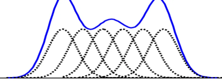
density function is formed by averaging of the kernel function values (see Figure 2).

Figure 2: Probability density function of a random variable and some Gaussian kernels This estimator is governed by the smoothing parameter ℎ called window width. Under some non-binding restrictions on ℎ, the Parzen window estimator is consistent. It exists several kernel functions (Gaussian, box, triangle…) but the Parzen window performances depend mainly on the choice of the window width ℎ. It exists several methods to choose ℎ. In this study, a Gaussian kernel has been used according to Eq. (12). Silverman [29] has determined an optimal window width value used a so-called “rule of thumb” when the distribution is Gaussian. This window width depends on an estimation of the variance 𝜎̂ and the learning data set size 𝑁 according to Eq. (13).

𝐾(𝑥) = 1 √2𝜋×𝑒 (𝑥_{2 )}2 (12) ℎ = 𝜎̂ ( 4 3×𝑁) 1 3 (13)

3.2 Estimation of the decision threshold for damage detection

According to the nonparametric Parzen window probability density function, 𝑓̂𝑁,ℎ, presented above in

Eq. (11), and after the choice of the window width ℎ using Eq. (13), the decision threshold, 𝑆PAR(PFA, 𝑁), may be determined according to a requested probability of false alarm (PFA) and given a

learning sample size 𝑁 using Eq.(14).

𝑆_PAR(PFA, N) = {𝑆 such that ∫ 𝑓̂𝑁,ℎ(𝑥)𝑑𝑥 =

1 𝑁ℎ∑ ∫ 𝐾 ( 𝑥 − 𝑥𝑖 𝑥 ) +∞ 𝑆 𝑁 𝑖=1 𝑑𝑥 = +∞ 𝑆 PFA} (14)

9

Eq. (14) thus provides an alternative to Eq. (10) to compute the decision threshold that theoretically corresponds to a given PFA, for a given learning sample size 𝑁. However, one should note that there is in Eq. (10) an additional parameter that corresponds to the learning threshold 𝑢. The performances of these two decision thresholds will now be assessed experimentally.

4 Experimental setup

4.1 Composite Aircraft Structures under study

The part of the nacelle we are interested in is the fan cowl. (see Figure 3). This structure is geometrically complex and is made of composite monolithic carbon epoxy. It is a multilayered structure consisting of two kinds of materials: certain parts are made of 3 plies oriented along [0°/ 45°/0°] and other parts of 4-plies oriented along [0°/ 45°/ -45°/ 0°]. This structure is 2.20 m in height for a semi-circumference of 5.80 m.

A network of 30 piezoelectric elements used as actuators and sensors has been bonded to the surface of the fan cowl and is used to emit and collect signals. The PZT elements used are numbered from 1 to 30 and mounted at specific positions on the composite plate’s surface as shown in Figure 3. The PZT elements have a diameter of 20 mm, a thickness of 0.1 mm and have been manufactured by Noliac.

Three types of damage are considered in that study. All the damages are located at the position of the red cross shown in Figure 3. The first two damages are made using Neodymium magnets placed on both sides of the fan cowl (see Figure 3). Damage 1 is realized with a 45 mm magnet and damage 2 using the superposition of a 45 mm and a 40 mm magnets. Finally damage 3 is a 6 mm hole done with a driller within the structure (see Figure 3).

Figure 3 : Left: overview of the nacelle fan cowl. Blue circles with numbers denote the PZT elements and the red cross stands for the damage position. Right top: 45 mm Neodymium magnet. Right

bottom: zoom on the 6 mm hole.

4.2 Damage detection methodology

The methodology proposed for the detection of the damage appearing on the nacelle structure is summarized in Figure 4. This methodology consists of two main phases (training phase and testing phase). The “data pre-processing” and “damage index computation” steps common to both phases will be presented in Sections 4.3 and 4.4. The “decision statistic” and “decision threshold estimation” steps

10

correspond to the two detector design methodologies presented in Sections 2 and 3 that will be compared here.

Figure 4: Damage detection methodology.

4.3 Data preprocessing

Structural health monitoring is achieved here by means of Lamb waves [7]. This method is based on the principle that Lamb waves can propagate in the structure and will thus necessarily interact with damage. Information is then extracted from the waves diffracted by the damage for detection purposes. The excitation signal sent to the PZT element is a 5 cycles "burst" with a central frequency of 200 kHz and with an amplitude of 10 V. This signal has been chosen here in order to maximize the propagation of the 𝑆₀ mode. In each phase of the experimental procedure, one PZT is selected as the actuator and the other act as sensors. All the PZTs act sequentially as actuators. Resulting signals are then simultaneously

11

recorded by the others piezoelectric element and consist of 1000 data points sampled at 1 MHz. Given the fact that the Lamb wave propagation speed within the material is around 5200 m/s for the 𝑆₀ mode this thus correspond to a propagation distance of 5.2 m which is roughly the extent of the structure under study. For all configurations several repetitions are performed in order to have enough data for a statistical approach. An overview of the experimental campaign that has been carried out is given in Table 1.

As pre-processing steps, the measured signals are first denoised by means of a discrete wavelet transform up to the order 4 using the “db40” wavelet. Those signals are then filtered around their center frequency using a continuous wavelet transformation based on “morlet” wavelets and with a scale resolution equals to 20. The diaphonic part present in the measured signals (i.e. the copy of the input signals that appears on the measured signal due to electromagnetic coupling in wires) has been previously eliminated on the basis of the knowledge of the geometrical positions of the PZT and of the waves propagation speed in the material.

Configuration Number of repetitions Number of DIs

Healthy 𝑁_𝐻 = 1000 𝑁𝐻(𝑁𝐻− 1)

2 = 499500

Damage 1 (45 mm magnet) 𝑁₁ = 100 𝑁_𝐻×𝑁₁ = 105

Damage 2 (45 and 40 mm magnets) 𝑁₂ = 100 𝑁_𝐻×𝑁₂ = 105

Damage 3 (6 mm hole) 𝑁₃ = 1000 𝑁_𝐻×𝑁₃ = 106

Table 1 : Overview of the experimental campaign

4.4 Damage Index (DI) computation

The damage index represents a crucial step for the design of the detector as this feature must correctly reflect the effect of the damage on the structure. The damage index chosen for this study is obtained as follows given a reference healthy signal 𝑥(𝑡) and a signal 𝑦(𝑡) corresponding to an unknown state:

1) Both signals are oversampled by a factor 5.

2) Signals are time-aligned to compensate for any subsample time-misalignment that could have occurred during the acquisition. Excitation signals are taken as references to estimate the time misalignment between both states.

3) The difference between the oversampled signals Δ(𝑡) = 𝑥(𝑡) − 𝑦(𝑡) is computed. 4) The envelope of the difference 𝐸𝑁𝑉[Δ](𝑡) is computed thanks to a Hilbert transform. 5) The envelope of the reference healthy signal 𝐸𝑁𝑉[𝑥](𝑡) is computed the same way. 6) The damage index is computed as in Eq. (15).

𝐷𝐼𝑥𝑦 = √

∫ (𝐸𝑁𝑉[Δ](𝑡))₀𝑇 2𝑑𝑡 ∫ (𝐸𝑁𝑉[𝑥](𝑡))₀𝑇 2𝑑𝑡

12

By rotating the reference healthy signal and the signal corresponding to an unknown state (healthy or damaged), important DI-databases are obtained as shown in Table 1. Among these different databases, the one obtained by comparing the healthy set to itself is very interesting as it allows characterizing the healthy behavior of the structure and to compute the decision thresholds. This database will be the input of the two detector design methodologies presented in Sections 2 and 3 that will be compared here. Eq. (14) and Eq. (10) will thus be used to compute the two decision thresholds 𝑆_PAR(𝑁, PFA) and 𝑆_POT(𝑁, 𝑢, PFA) that theoretically correspond to a given PFA, for a given learning sample size 𝑁, and for a given learning threshold 𝑢 (only in the 𝑆_POT case). As an example, Figure 5 represents the histograms of the DI for the actuator 1 – sensor 8 path for the different healthy and damaged cases (see Table 1).

Figure 5: Example of histograms for the healthy and damaged cases (see Table 1) for the path with actuator 1 and sensor 8.

The path actuator 1 – sensor 8 is relatively close to the damage, but not directly exposed to the damage (as may be for example the path actuator 2 – sensor 5, see Figure 3). This makes it particularly interesting in the present context. Furthermore, it can be seen in Figure 5 that even if not directly including the damage, this path can still provide DIs that differs greatly between the healthy and damage states. Additionally, results for the other paths near the damage are qualitatively comparable to the results obtained for the path actuator 1 – sensor 8. For those reasons, this path will be used in the following as an illustrative example of the obtained results.

13

5 Analysis of the performances of the POT-based and PARZEN-based detectors

The two detector design methodologies presented in Sections 2 and 3 are now compared here. Eq. (14) and Eq. (10) are used to compute the two decision thresholds 𝑆_PAR(𝑁, PFA) and 𝑆_POT(𝑁, 𝑢, PFA) that theoretically correspond to a given desired PFA for a given learning sample size 𝑁. The performances of these two decision thresholds will be assessed experimentally in the following after discussing the fit quality between the experimentally obtained data and the retained model as well as the choice of the minimal learning thresholds 𝑢_𝑚𝑖𝑛 necessary to compute 𝑆_POT.

5.1 Validation of the Generalized Pareto Distribution (GPD) assumption

As explained in Section 2, it is assumed here that the tail of the DI distribution above a certain threshold 𝑢 can be modeled as a GPD. The aim of this section is thus to assess that the tail of the experimentally obtained DIs can effectively be modeled by a GPD above a certain minimal threshold 𝑢_𝑚𝑖𝑛 and to estimate the order of magnitude of this minimal threshold.

Figure 6: [Left] Mean Excess Function for DIs for the healthy case for the path 1 to 8. [Right] Q-Q plot comparing the experimental data and the fitted GPD model.

In order to do so, two statistical tools can be used. The first one is the ME-plot that has been introduced in Section 2.4. Given a ME-plot, it is possible to estimate the value of the threshold 𝑢𝑚𝑖𝑛

above which the empirical tail can be approximated by a GPD. Indeed, 𝑢𝑚𝑖𝑛 corresponds to the value

of 𝑢 above which the mean excess function, 𝑒(𝑢), decreases linearly. The ME-plot for the DIs computed for the path between the actuator 1 and the sensor 8 is plotted on the left part of Figure 6. According to this figure, it can be observed that above a value 𝑢_𝑚𝑖𝑛 = 3.75 (which corresponds to the 4.9% highest DIs) the behavior of 𝑒(𝑢) is almost linear. Furthermore, it is noticeable that the slope of 𝑒(𝑢) is negative above 𝑢_𝑚𝑖𝑛. According to Eq. (9), this slope is proportional to the GPD parameter 𝜉. As this slope is negative, the value of 𝜉 is thus negative for the experimentally obtained DIs. This implies that the corresponding Domain of Attraction of the Maximum (DAM) for this set of data is of Weibull type (see Figure 1). After fitting a GPD to the tail of the experimental data, it is possible to make use of a QQ-plot in order to assess the fitted model quality. A QQ-plot displays the samples from the experimental data versus the samples from the fitted GPD. If all the points of the QQ-plot lie on the diagonal, this means that the fitted model describes the experimental data

14

correctly. The QQ-plot for the DIs above 𝑢_𝑚𝑖𝑛 computed for the path between the actuator 1 and the sensor 8 and for the fitted GPD with 𝜉 = −0.13752 and 𝛽 = 0.13306 is plotted on the right part of Figure 6. The conclusion that the estimated GPD describes correctly the tail of the experimental data can easily be drawn from this figure.

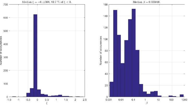
The same procedure for the estimation of the GPD parameters have been repeated for all the 29×30 = 870 paths available all over the structure (see Figure 3) when retaining 5% of the highest DIs. The empirical distribution of these parameters is shown in Figure 7. From this figure, it can be observed that 83.7% of the paths have been modeled using a negative value for 𝜉. This means that the majority of the domain of attraction observed experimentally are of Weibull type (see Figure 1).

Furthermore, it can be observed that the values of the parameter 𝛽 span a rather wide range within the structure. In order to illustrate that, Figure 8 displays the Q-Q plots for the paths for which the value of β was very small, the value of β was very large, the value of ξ was very low, and the value of ξ was positive. From this figure, it can be seen that even under rather large variations of the parameters

𝛽 and 𝜉, the fit of the data with a GPD is still very good. In conclusion of this section it can be said

that the tail of the experimentally obtained DIs can effectively be modeled by a Weibull-type DAM GPD above a minimal threshold 𝑢𝑚𝑖𝑛 that retains ≃ 5% of the highest DIs.

Figure 7: Distribution of the estimated GPD parameters 𝜉 [Left] and 𝛽 [Right] over the 870 paths available over the whole structure when retaining 5% of the highest DIs.

15

Figure 8 : Q-Q plot comparing the experimental data and the fitted GPD model for different values of the parameters 𝜉 and 𝛽. [Top left] Small value of 𝛽. [Top right] Positive value of 𝜉. [Bottom left]

Small value of 𝜉. [Bottom right] Large values of 𝜉 and 𝛽.

5.2 Comparison between decision thresholds obtained using both methods

Now that it appears clear that it makes sense to model the tails of the experimentally obtained DIs using GPD, it is possible to compare the detection thresholds issued by the two methodologies described in Section 2 and Section 3. Eq. (14) and Eq. (10) will thus be used to compute the two decision thresholds 𝑆_PAR(𝑁, PFA) and 𝑆_POT(𝑁, 𝑢, PFA) that theoretically correspond to a given PFA, for a given learning sample size 𝑁, and for a given learning threshold 𝑢 (only in the 𝑆_POT case). As the design of the detection threshold based on Parzen windows is more classical, it will be considered here as a reference. But this does not mean that the thresholds obtained through this approach constitute the ground truth which is totally unknown here. Then, in order to compare the two thresholds, the threshold relative difference (Δ(𝑁, 𝑢, PFA) in %) defined as in Eq. (16) will be used.

Δ(𝑁, 𝑢, PFA) = 100×𝑆POT(𝑁, 𝑢, PFA) − 𝑆𝑃𝐴𝑅(𝑁, 𝑃𝐹𝐴) 𝑆𝑃𝐴𝑅(𝑁, 𝑃𝐹𝐴)

16

Figure 9: Threshold relative difference as a function of the percentage of data retained for learning for several PFA and using all 100% of the available samples [Left] or only 20% of the available

samples [Right].

The threshold relative difference Δ(𝑁, 𝑢, PFA) as a function of the percentage of data retained for learning (proportional to 𝑢) for several PFA and using all 𝑁 = 100% of the available samples [Left] or only 𝑁 = 20% of the available samples [Right] is plotted in Figure 9 for different desired PFA ranging from 10−4 _{to 10}−9_{. From this figure, it can be seen that for large values of the desired}

PFA the threshold relative difference is rather low (≃ 1 − 2%), which means that the thresholds provided by the two methodologies are pretty similar. However, this is not at all the case for the smaller values of the PFA for which the threshold relative difference can reach up to 12%. This is due to the fact that with the GPD, a more precise, and thus different, model of the tail is estimated than with the Parzen windows. The difference between the left part and the right part of Figure 9 lies in the fact that the number of samples that has been used for threshold estimation is different: 𝑁 = 100% of the samples for the left part and 𝑁 = 20% of the samples for the right part. By comparing these two figures, it can be seen that the overall shape of the curves is similar but that the vertical scale is not the same (maximum around 8% on the left and around 12% on the right). Indeed, when a smaller number of samples is available, the difference between the two estimated thresholds becomes larger. The reason for that is that with fewer samples, the design method based on the GPD ends up with less samples above the learning threshold 𝑢 and thus with a less precise estimation of the tail model, especially when very low PFA are desired.

17

Figure 10: Threshold relative difference as a function of the percentage of data retained for learning for several proportions of the available samples 𝑁 and for a PFA= 10−5 _{[Left] and 10}−8 _[Right].

In order to analyze the results with a different focus, the threshold relative difference Δ(𝑁, 𝑢, PFA) as a function of the percentage of data retained for learning for several proportions of the available samples 𝑁 and for a PFA= 10−5 _{[Left] and 10}−8 _{[Right] is plotted on Figure 10. From this figure, it}

can be seen that all curves are globally decreasing. This means that whatever the number of available samples, the smaller the number of samples retained for learning (i.e. the larger 𝑢) the better the agreement is between both design methodologies. Furthermore, it can be noticed that, as already seen in Figure 9, as the PFA becomes smaller the disparity increases between the two thresholds. And by comparing Figure 9 and Figure 10, one can finally see that the PFA has a large and easily interpretable influence on Δ(𝑁, 𝑢, PFA) whereas it is not the case for 𝑁 that appears to be less influent.

In summary, this section illustrates the fact that differences up to ≃ 10% can exist between the thresholds estimated by the two methods. Those differences however reduce significantly (up to ≃ 1%) if the PFA is large enough or if the number of samples retained to learn the GPD is small enough (or equivalently if the threshold 𝑢 is high enough). Additionally, the number of samples 𝑁 seems to be a much less influent parameter than the PFA.

5.3 Reliability with respects to the desired PFA

In the previous section, the differences existing between the two threshold design methodologies have been highlighted. However, it is still not possible to assess which one of the two thresholds can be considered as more reliable than the other. The aim of this section is to do so by taking into account the fact that the only input design data that is fed to both methodologies is a “desired” PFA. As here, numerous experimental data are available; it is thus possible to compute the “effective” PFA

18

(that is the PFA that is obtained using the experimental DIs with a given threshold) and to compare it to the “desired” PFA. It will then possible to assess which threshold is the best accordingly to this objective criterion.

Figure 11: Effective PFA for the path Actuator 1 – Sensor 8 as a function of the percentage of data retained for learning for several proportions of the available samples 𝑁 and for a desired PFA=

10−4_{. Solid lines are obtained using thresholds 𝑆}

POT and dashed lines using thresholds 𝑆PAR.

The effective PFA for the path Actuator 1 – Sensor 8 as a function of the percentage of data retained for learning for several proportions of the available samples 𝑁 is plotted for a desired PFA of 10−4 _{on Figure 11 and for a desired PFA of 10}−5 _{on Figure 12. The solid lines are obtained using}

thresholds 𝑆POT and the dashed ones using thresholds 𝑆PAR. Additionally, the desired PFA is also

reported by means of a thicker black line. From these figures it can first be seen that the thresholds estimated using Parzen windows always provide effective PFA that are lower than the desired ones. In that sense the design methodology can be qualified as “conservative”. This is due to the fact that the methodology based on Parzen windows makes use of all the available data and thus that the data that do not belong to the tail weights more than the data that belongs to the tails (that unfortunately conveys the most interesting information). This is not true for the thresholds designed using the GPD approach. For those thresholds the effective PFA can be higher or lower than the desired PFA. Furthermore, for the GPD based thresholds, one can notice that their effective PFA converge towards the desired PFA as the learning threshold 𝑢 becomes higher. This is consistent with the fact that as the learning threshold becomes higher, the GPD assumption become more valid and thus the fitted model describes the experimental DIs in a better way. Finally, one can notice that the number of sample 𝑁 does not seem here to be very influent.

19

Figure 12: Effective PFA as a function of the percentage of data retained for learning for several proportions of the available samples 𝑁 and for a desired PFA= 10−5_{. Solid lines are obtained using}

thresholds 𝑆POT and dashed lines using thresholds 𝑆PAR.

As the structure under study is equipped with 30 piezo-electric elements (see Figure 3), this analysis of “desired PFA” versus “effective PFA” can be performed for all the 30×29 = 870 paths available over the structure. The effective PFA computed for all the paths of the structure as a function of the percentage of data retained for learning for several proportions of the available samples 𝑁 and for a desired PFA of 10−5 _{is plotted on Figure 13. Again, the solid lines are obtained}

using thresholds 𝑆_POT, the dashed ones using thresholds 𝑆_PAR, and the desired PFA is reported by means of a thicker black line. This figure synthesizing results for the entire structure confirms that the thresholds estimated using Parzen windows always provide effective PFAs that are lower than the desired ones and can thus be qualified as “conservative”. This is not true for the thresholds designed using the GPD approach that provides effective PFAs observed to be slightly higher than the desired PFA. One can again notice that for these thresholds their effective PFA converge towards the desired PFA as the learning threshold 𝑢 becomes higher. Finally, one can notice that as the number of sample 𝑁 increases, the effective PFA become closer to the desired one, a fact that was not observable in Figure 11 and Figure 12 due to the lower number of samples available for PFA computation.

20

Figure 13: Effective PFA averaged over all the possible paths as a function of the percentage of data retained for learning for several proportions of the available samples 𝑁 and for a desired PFA=

10−5_{. Solid lines are obtained using thresholds 𝑆}

POT and dashed lines using thresholds 𝑆PAR.

To sum it up, this section highlights the fact that thresholds designed using the Parzen windows approach are very conservative and will produce an effective PFA that is always lower than the desired one. Furthermore, the effective PFA produced by the thresholds designed using the GPD approach are closer to the desired PFA as long as the GPD assumptions are valid (i.e. as long as the learning threshold 𝑢 is high enough). Additionally, the number of samples 𝑁 seems to be a parameter with a lower influence.

5.4 Detection performances

As the main objective of the present study is to design a detector for structural health monitoring purposes, it is also mandatory to evaluate the performances of the detector in terms of probability of detection (PoD). Indeed, a common approach in detector design is to level up the detection threshold in order to minimize the PFA, as effectively done here. However, when doing so it may be possible that the retained threshold is so high that is falls within the range where DIs values in any damaged case are expected. In that case, the detector design ensures a very low PFA but at the cost of a significant reduction of performances in terms of PoD which is not acceptable in practice.

21

Figure 14: Histograms for the healthy and damaged cases (see Table 1) for the path with actuator 1 as well as thresholds obtained using the Parzen and Pareto methods. The thresholds are obtained for a PFA of 10−9_{, 𝑁 = 100% of the sample retained and a learning threshold 𝑢 for the}

Pareto method such that 5% of the extremal data are considered.

Figure 14 presents the histograms for the healthy and damaged cases (see Table 1) for the path with actuator 1 and sensor 8 as well as thresholds obtained using the Parzen and Pareto methods. These thresholds are obtained for a PFA of 10−9, 𝑁 = 100% of the sample retained and a learning threshold 𝑢 for the Pareto method such that 5% of the extremal data are considered. On that figure, it can clearly be seen that the threshold provided by the two methods given the same input PFA can greatly differ, as highlighted in Section 5.2. However, il also highlights the fact that in the present case the choice of a very low PFA (equal to 10−9 here) is not detrimental to the detection quality. Indeed, for both detectors, the probability of detection still remains almost equal to one for the three damage cases considered here. This is due here to the fact that the DIs distribution between the healthy and damaged states are sufficiently well separated that it is possible to increase the detection threshold value without compromising damage detection.

5.5 Discussion

The results provided in the previous sections allow concluding that the estimated GPD describes correctly the tail of the experimental data when retaining ≃ 5% of the highest DIs. When designing threshold using both the Parzen windows approach and the GPD approach, differences can exist

22

between the thresholds estimated by the two methods. Those differences, however, reduce significantly if the PFA is large enough or if the number of samples retained to learn the GPD is small enough. Furthermore, thresholds designed using the Parzen windows approach are very conservative whereas PFA produced by the thresholds designed using the GPD approach are closer to the desired PFA as long as the GPD assumptions are valid. Additionally, the number of samples 𝑁 seems to be a parameter with less influence.

By focusing more specifically on the design methodology based on Parzen windows, it clearly has some advantages and drawbacks. First, this design methodology has been shown to be very conservative in terms of effective PFA. This could be an advantage from an industrial perspective as long as the cost of a false alarm is higher than the cost of non-detection. This is clearly a drawback if it is not the case. Another point that should be considered is that the proposed design methodology is nonparametric. As for real life applications, no knowledge about the DIs distribution is available, this design methodology can face many different practical cases. Finally, a drawback of this methodology is that it relies on the entire DIs database and thus can induce costly and timely computations when large databases are available.

By focusing now on the design methodology based on GPD, it also has some advantages and drawbacks. One of its advantages is that it is accurate in the sense that the effective PFA is close to the desired PFA as long as the GPD assumptions are valid. With that methodology, industrials can thus be more confident with the PFA realized by their monitoring equipment. However, this methodology is only semiparametric. Indeed, it still relies on parametric expressions of the GPD. Nevertheless, this cannot be considered as a real drawback as the GPD parameters can be automatically estimated. Finally, an advantage of this methodology is that it relies on DIs higher than a certain threshold and thus computations can be done more easily and rapidly.

In any case, one should keep in mind that the only data that are necessary to estimate thresholds using these two methodologies are the data in the healthy state of the structure. By definition, these data are widely available and thus using in practice these algorithms seems to be something realistic from an industrial perspective. This makes both algorithms interesting from a practical point of view. In order to deploy them for practical applications, the following questions must, however, be answered: How many samples do we need? Which method to choose? Regarding the number of samples, as they are “free” in the sense that there is no need to damage a structure to acquire them, it appears that the more is the better. However, this point can be mitigated by saying that the number of samples did not appear to be a very influent parameter in the present study. Regarding the method to retain, it depends. Indeed, the choice of the method to retain will largely depends on the available number of samples and on the desired PFA. And finally regarding the confidence with respect to effective PFA, what can be said is that the designed detection threshold will be accurate using the GPD-based approach if the learning threshold is correctly chosen and that the threshold will be conservative using the Parzen window approach.

23

6 Conclusion

Structural Health Monitoring (SHM) offers new approaches to interrogate the integrity of complex structures. The SHM process relies on four sequential steps: damage detection, localization, classification, and quantification. The most critical step of such process is the damage detection step since it is the first one and because performances of the following steps depend on it. The detector used in that step relies on a decision threshold computed from a statistical characterization of the damage indexes available in the healthy behavior of the structure. In this study we modeled the tail of the decision statistics (which is defined here as the Damage Index distribution) using the Peaks Over Threshold method extracted from the Extreme Value Theory in order to determine the decision threshold corresponding to a given PFA. This methodology has been applied in the context of a composite aircraft nacelle for different configurations of learning sample size and PFA and compared to a more classical one which consists in modelling the whole distribution by means of Parzen windows. The first aim of the study was to investigate the potential of the POT method to estimate the parameters of the tail statistical model as well as the effect of design parameters such as the total number of samples or the percentage of higher samples retained for learning. The second aim of the study was to make use of industrially coherent PFA ranging from 10−4 _{to 10}−9 _{and to assess the validity of the proposed threshold design methodology with respect}

to the desired PFA. The results provided by this study allow concluding that the estimated GPD describes correctly the tail of the experimental data when retaining ≃ 5% of the highest DIs. When designing threshold using both the Parzen windows approach and the GPD approach, differences can exist between the thresholds estimated by the two methods. Those differences however reduce significantly if the PFA is large enough or if the number of samples retained to learn the GPD is small enough. Furthermore, thresholds designed using the Parzen windows approach are very conservative whereas PFA produced by the thresholds designed using the GPD approach are closer to the desired PFA as long as the GPD assumptions are valid. Additionally, the number of samples seems to be a parameter with no real influence as long as it is large enough.

7 Acknowledgments

This work was partially supported by the CORALIE project: CORAC/EPICE-AP2-P6-07/CORALIE. The authors also would like to thank SAFRAN NACELLE for providing the aeronautical structure.

[1] K. Worden and J. Dulieu-Barton, "An overview of intelligent fault detection in systems and structures," Structural Health Monitoring, vol. 3, no. 1, pp. 85-98, 2004.

[2] D. Balageas, C.-P. Fritzen and A. Guemes, Structural health monitoring, vol. 493, Wiley Online Library, 2006.

[3] F.-K. Chang, Structural Health Monitoring 2003: From Diagnostics & Prognostics to Structural Health Management: Proceedings of the 4th International Workshop on Structural Health Monitoring, Stanford University, Stanford, CA, September 15-17, 2003, DEStech Publications, Inc, 2003.

24

[5] W. Staszewski, C. Boller and G. R. Tomlinson, Health monitoring of aerospace structures: smart sensor technologies and signal processing, John Wiley & Sons, 2004.

[6] C. R. Farrar and K. Worden, "An introduction to structural health monitoring," Philosophical Transactions of the Royal Society of London A: Mathematical, Physical and Engineering Sciences, vol. 365, no. 1851, pp. 303-315, 2007.

[7] Z. Su and L. Ye, Identification of damage using Lamb waves: from fundamentals to applications, vol. 48, Springer Science & Business Media, 2009.

[8] O. Hmad, N. Mechbal and M. Rebillat, "Peaks Over Threshold Method for Structural Health Monitoring Detector Design," in Proceedings of the International Workshop on Structural Health Monitoring, 2015.

[9] C. M. S. Kabban, B. M. Greenwell, M. P. DeSimio and M. M. Derriso, "The probability of detection for structural health monitoring systems: Repeated measures data," Structural Health Monitoring, p. 1475921714566530, 2015.

[10] O. Hmad, P. Beauseroy, E. Grall-Maes, A. Mathevet and J. R. Masse, "A comparison of distribution estimators used to determine a degradation decision threshold for very low first order error," Advances in Safety, Reliability and Risk Management: ESREL 2011, p. 59, 2011.

[11] N. L. Hjort and M. Jones, "Locally parametric nonparametric density estimation," The Annals of Statistics, pp. 1619-1647, 1996.

[12] O. Hmad, E. Grall-Maes, P. Beauseroy, J. Masse and A. Mathevet, "Maturation of Detection Functions by Performances Benchmark. Application to a PHM Algorithm," in Prognostics and System Health Management Conference, 2013.

[13] A. A. Balkema and L. De Haan, "Residual life time at great age," The Annals of probability, pp. 792-804, 1974.

[14] S. Coles, J. Bawa, L. Trenner and P. Dorazio, An introduction to statistical modeling of extreme values, vol. 208, Springer, 2001.

[15] J. Pickands, "Statistical inference using extreme order statistics," The Annals of Statistics, pp. 119-131, 1975.

[16] E. J. Gumbel, Statistics of extremes, Courier Corporation, 2012.

[17] J. R. Hosking and J. R. Wallis, "Parameter and quantile estimation for the generalized Pareto distribution," Technometrics, vol. 29, no. 3, pp. 339-349, 1987.

[18] L. De Haan and A. Ferreira, Extreme value theory: an introduction, Springer Science \& Business Media, 2007.

[19] R. O. Duda, P. E. Hart and D. G. Stork, Pattern classification, John Wiley & Sons, 2012. [20] H. Rootzén and N. Tajvidi, "Extreme value statistics and wind storm losses: a case study,"

Scandinavian Actuarial Journal, vol. 1997, no. 1, pp. 70-94, 1997.

[21] H. Sohn, D. W. Allen, K. Worden and C. R. Farrar, "Structural damage classification using extreme value statistics," 2005.

[22] K. Worden, G. Manson, H. Sohn and C. Farrar, "Extreme value statistics from differential evolution for damage detection," in Proceedings of the 23rd international modal

25 analysis conference (IMAC XXIII), 2005.

[23] Z. Li and Y. Zhang, "Extreme value theory-based structural health prognosis method using reduced sensor data," Structure and Infrastructure Engineering, vol. 10, no. 8, pp. 988-997, 2014.

[24] H. W. Park and H. Sohn, "Parameter estimation of the generalized extreme value distribution for structural health monitoring," Probabilistic Engineering Mechanics, vol. 21, no. 4, pp. 366-376, 2006.

[25] R. A. Fisher and L. H. C. Tippett, "Limiting forms of the frequency distribution of the largest or smallest member of a sample," in Mathematical Proceedings of the Cambridge Philosophical Society, 1928.

[26] B. P. Rao, Nonparametric functional estimation, Academic press, 2014.

[27] L. De Haan and H. Rootzén, "On the estimation of high quantiles," Journal of Statistical Planning and Inference, vol. 35, no. 1, pp. 1-13, 1993.

[28] E. Parzen, "On estimation of a probability density function and mode," The Annals of Mathematical Statistics, vol. 33, no. 3, pp. 1065-1076, 1962.

[29] B. W. Silverman, Density estimation for statistics and data analysis, vol. 26, CRC press, 1986.