Science Arts & Métiers (SAM)
is an open access repository that collects the work of Arts et Métiers Institute of
Technology researchers and makes it freely available over the web where possible.
This is an author-deposited version published in: https://sam.ensam.eu
Handle ID: .http://hdl.handle.net/10985/8486
To cite this version :
Adil EL BAROUDI, Fulgence RAZAFIMAHERY - Three-dimensional investigation of the stokes eigenmodes in hollow circular cylinder - Advances in Acoustics and Vibration - Vol. 2013, n°857821, p.1-15 - 2013
Any correspondence concerning this service should be sent to the repository Administrator : [email protected]
Three-Dimensional Investigation of the Stokes Eigenmodes in
Hollow Circular Cylinder
Adil El Baroudi
1and Fulgence Razafimahery
21Arts et M´etiers ParisTech, ENSAM Angers, 2 Boulevard du Ronceray, 49035 Angers, France 2IRMAR, Universit´e de Rennes 1, Campus de Beaulieu, 35042 Rennes Cedex, France
Correspondence should be addressed to Adil El Baroudi; [email protected]
This paper studies the influence of boundary conditions on a fluid medium of finite depth. We determine the frequencies and the modal shapes of the fluid. The fluid is assumed to be incompressible and viscous. A potential technique is used to obtain in three-dimensional cylindrical coordinates a general solution for a problem. The method consists in solving analytically partial differential equations obtained from the linearized Navier-Stokes equation. A finite element analysis is also used to check the validity of the present method. The results from the proposed method are in good agreement with numerical solutions. The effect of the fluid thickness on the Stokes eigenmodes is also investigated. It is found that frequencies are strongly influenced.
1. Introduction
Flow modeling in confined domains leads mostly to Stokes models [1]. The use of this model in the field of microflu-idics and nanoflumicroflu-idics [2, 3] and in the understanding the movement of microorganisms [4] currently in full swing. This recent years, several authors have focused on the modal anal-ysis of this model. We can cite in particular the aspects related to problems arising from geophysics. These studies highlight the existence of slow wave or Stoneley waves [5–7]. Other authors [8,9] have focused on the dynamic aspects in the con-text of fluid-structure interaction. The numeric aspects for coupled (or not) modal problem were discussed in [10–12].
The theory of potential flow of viscous fluid was intro-duced by [13]. All of his work on this topic is framed in terms of the effects of viscosity on the attenuation of small ampli-tude waves on a liquid-gas surface. The problem treated by Stokes was solved exactly using the linearized Navier-Stokes equations, without assuming potential flow, and was solved exactly by [14]. Reference [15] has identified the main events in the history of thought about potential flow of viscous fluids. The problem of Stokes flow in cylindrical domain has been investigated by several authors. References [16, 17] studied
Stokes flow in a cylindrical container by an eigenfunction expansion procedure without the compressibility effect.
Potential flows through different kinds of geometry have been studied by many investigators for several applications. For example in vascular fluid dynamics, [18] presented the role of curvature in the wave propagation and in the develop-ment of a secondary flow. Reference [19] has studied the flow and pressure dynamics of the cerebrospinal fluid flow. Three-dimensional CSF flow studies have also been reported [20].
The knowledge of Stokes eigenmodes in a three-dimen-sional confined domain, in a square/cube [10], or in any bounded domain could provide some insight into the under-standing or analysis of turbulent instantaneous flow field in a geometry as simple as, for instance, the driven cavity.
This paper deals with analytical and numerical modeling of three-dimensional incompressible viscous fluid using the potential technique and the finite element method. The ana-lytical formulation is based upon a convenient decomposition of the velocity field into two contributions [9–21]: one is related to the scalar potential and the other is the vector potential.
The rest of the paper is organized as follows. In Section
representation for the velocity field in terms of the potential. The implementation of analytical solutions is discussed in detail.Section 3describes boundary condition treatment for modeling Stokes eigenmodes.Section 4investigates the case of fluid-solid interaction.Section 5is completely devoted to the analytical and numerical results. Finally, the paper is ended by some conclusions.
2. Governing Equations
From conservations of mass and momentum and assuming that the fluid is viscous and incompressible, the motion of the fluid flowing in the cylindrical waveguide in the absence of body force is governed by
𝜌𝜕v (𝑟, 𝜃, 𝑧)
𝜕𝑡 = −∇𝑝 (𝑟, 𝜃, 𝑧) + 𝜂∇
2v (𝑟, 𝜃, 𝑧) , (1)
∇ ⋅ v (𝑟, 𝜃, 𝑧) = 0, (2)
in whichv(𝑟, 𝜃, 𝑧) = {V𝑟, V𝜃, V𝑧}𝑇(𝑟, 𝜃, 𝑧) is the fluid velocity vector,𝑝(𝑟, 𝜃, 𝑧) is the fluid pressure, 𝜌 is the density of the fluid, and] and 𝜂 = 𝜌] are the kinematic and dynamic fluid viscosity, respectively.
The obtained equations of motion are highly complex and coupled. However, a simpler set of equations can be obtained by introducing scalar potentials𝜙, 𝜓, and 𝜒, known as the Helmholtz decomposition. The Helmholtz decomposition theorem [22] states that any vectorv can be written as the sum of two parts: one is curl-free and the other is solenoidal. In flow fields, the velocity is thereby decomposed into a potential flow and a viscous flow. In other words, the velocityv can be decomposed into the following form:
v = ∇𝜙 + ∇ × (𝜓ez) + ∇ × ∇ × (𝜒ez) , (3)
whereezis the unit vector along the𝑧 direction. Substituting the above resolutions into (1) and (2), after some manipula-tions, the equation for the conservation of mass (2) becomes the Laplace equation:
∇2𝜙 (𝑟, 𝜃, 𝑧) = 0, (4)
and the equation for the conservation of momentum (1) becomes the Helmholtz equations
∇2𝜓 (𝑟, 𝜃, 𝑧) −1 ] 𝜕𝜓 (𝑟, 𝜃, 𝑧) 𝜕𝑡 = 0, ∇2𝜒 (𝑟, 𝜃, 𝑧) −1]𝜕𝜒 (𝑟, 𝜃, 𝑧)𝜕𝑡 = 0, (5) where∇2 = (𝜕2/𝜕𝑟2) + (1/𝑟)(𝜕/𝜕𝑟) + (1/𝑟2)(𝜕2/𝜕𝜃2) + (𝜕2/ 𝜕𝑧2) is the Laplacian operator in polar coordinates, and time dependence has the form exp(𝑗𝜔𝑡). The pressure can be pre-sented by
𝑝 = −𝜌𝜕𝜙
𝜕𝑡. (6)
Thus, the Navier-Stokes equations are reduced to formula-tions (4), (5), and (6). Of course, it does not mean that
in any case such a decomposition of fluid’s velocity field gives considerable simplifications in solving the problem because boundary conditions for stresses are not separated. The vibrations are harmonic, with constant angular frequency 𝜔; as a result all potentials components and pressure will depend on time only through the factor exp(𝑗𝜔𝑡).
Applying the method of separation of variables, the solution of the equations for potentials, associated with an axial wave number 𝑘𝑧, radial wave number 𝑘𝜓, and cir-cumferential mode parameter𝑛, after considerable algebraic manipulations, can be shown to be
𝜙 = [𝐴𝐼𝑛(𝑘𝑧𝑟) + 𝐵𝐾𝑛(𝑘𝑧𝑟)] {cossin(𝑛𝜃)(𝑛𝜃)} × {cos(𝑘𝑧𝑧) sin(𝑘𝑧𝑧)} , (7) 𝜓 = [𝐶𝐽𝑛(𝑘𝜓𝑟) + 𝐷𝑌𝑛(𝑘𝜓𝑟)] {cossin(𝑛𝜃)}(𝑛𝜃) × {cos(𝑘𝑧𝑧) sin(𝑘𝑧𝑧)} , (8) 𝜒 = [𝐸𝐽𝑛(𝑘𝜓𝑟) + 𝐹𝑌𝑛(𝑘𝜓𝑟)] {cossin(𝑛𝜃)(𝑛𝜃)} × {sin(𝑘𝑧𝑧) cos(𝑘𝑧𝑧)} . (9)
𝐽𝑛 and𝑌𝑛 are Bessel functions of the first and second kind
of order 𝑛. 𝐼𝑛 and 𝐾𝑛 are modified Bessel functions of the first and second kinds of order 𝑛. 𝑛 and 𝑘𝑧 are the azimuthal and axial wavenumbers.𝑛 = 0, 1, 2, . . ., whereas 𝑘𝑧 is found by satisfying the symmetry boundary condition
on the 𝑧 = 0 and 𝑧 = 𝑙. Note that the velocity field
v has components that are symmetric or antisymmetric in
𝜃 and 𝑧. Following standard practice, the solutions with symmetric (antisymmetric) axial velocities are called the antisymmetric (symmetric) axial modes, respectively, with 𝑘𝑎
𝑧and𝑘𝑠𝑧denoting the corresponding eigenvalues. Thus, we
have 𝑘𝑎𝑧 = (𝑚 − 1)𝜋/𝑙 and 𝑘𝑠𝑧 = 𝑚𝜋/𝑙 (𝑚 = 0, 1, 2, . . .). However, the azimuthal modes corresponding to cos(𝑛𝜃) and sin(𝑛𝜃) are really the same, due to periodicity in the azimuthal direction; that is, there is no distinction in the values of𝑛 for the two families.𝐴, 𝐵, 𝐶, 𝐷, 𝐸, and 𝐹 are unknown coefficients which will be determined later by imposing the appropriate boundary conditions. The radial wave number𝑘𝜓is related to the axial wave number𝑘𝑧by
𝑘2𝜓= 𝛼2− 𝑘2𝑧, 𝜔 = 𝑗]𝛼2, (10) where𝑗 = √−1. In the end, the pressure can be obtained by insertion of (7) into (6),
Using (3) and taking into account (7), (8), and (9), the fluid particle velocities in terms of the Bessel functions can be written as V𝑟= {𝐴𝐼𝑛(𝑘𝑧𝑟) + 𝐵𝐾𝑛(𝑘𝑧𝑟) −𝑛𝑟𝐶𝐽𝑛(𝑘𝜓𝑟) −𝑛𝑟𝐷𝑌𝑛(𝑘𝜓𝑟) + 𝑘𝑧𝐸𝐽𝑛(𝑘𝜓𝑟) + 𝑘𝑧𝐹𝑌𝑛(𝑘𝜓𝑟) } × sin (𝑛𝜃) cos (𝑘𝑧𝑧) , V𝜃= {𝑛𝑟𝐴𝐼𝑛(𝑘𝑧𝑟) +𝑛𝑟𝐵𝐾𝑛(𝑘𝑧𝑟) − 𝐶𝐽𝑛(𝑘𝜓𝑟) − 𝐷𝑌𝑛(𝑘𝜓𝑟) +𝑛𝑘𝑟𝑧[𝐸𝐽𝑛(𝑘𝜓𝑟) + 𝐹𝑌𝑛(𝑘𝜓𝑟)]} × cos (𝑛𝜃) cos (𝑘𝑧𝑧) , V𝑧= {𝑘2𝜓𝐸𝐽𝑛(𝑘𝜓𝑟) + 𝑘𝜓2𝐹𝑌𝑛(𝑘𝜓𝑟) − 𝑘𝑧𝐴𝐼𝑛(𝑘𝑧𝑟) −𝑘𝑧𝐵𝐾𝑛(𝑘𝑧𝑟) } sin (𝑛𝜃) sin (𝑘𝑧𝑧) . (12) In the following section we consider a fluid with different boundary conditions.
3. Boundary Conditions and
Frequency Equation
First we defineΓ1(𝑟 = 𝑅1), as the inner boundary of the fluid region, andΓ2 (𝑟 = 𝑅2), as the outer boundary. We begin the analysis of frequency equation for imposing the no-slip boundary conditions.
3.1. Stokes Eigenmodes in the Case of “No-Slip-No-Slip” Bound-ary Conditions. The no-slip hypothesis of fluid mechanics
states that liquid velocity at a solid surface is equal to the velo-city of the solid surface. Hence the no-slip boundary condi-tion can be written as
(1) the velocity is equal to zero atΓ1:
V𝑟= V𝜃= V𝑧= 0, (13)
(2) the velocity is equal to zero atΓ2:
V𝑟= V𝜃= V𝑧= 0. (14)
Combining these boundary conditions with (12) yields for each mode number(𝑛, 𝑚) the following linear system:
[M1] {𝑥} = {0} , {𝑥} = {𝐴 𝐵 𝐶 𝐷 𝐸 𝐹}𝑇, (15)
where[M1] is a 6 × 6 matrix whose components 𝑎𝑖𝑗are given inAppendix A. For a non-trivial solution, the determinant of the matrix[M1] must be equal to zero
det[M1] = 0. (16)
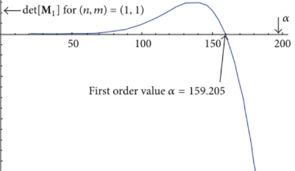
The roots of (16) give the natural frequencies 𝜔 of the cylindrical oscillations.Figure 16inAppendix Dshows ana-lytical calculation of eigenvalues𝛼 and using (10) we obtain the natural frequencies𝜔 [rd/s].
3.2. Stokes Eigenmodes in the Case of ”No-Slip-Normal Stress-Free” Boundary Conditions. The pressure and velocity
boundary conditions on the free surface are both formulated from the dynamic constraint of continuity of normal momen-tum flux across the free surface. The component of the stress tensor in the outward normal direction is therefore
𝜎 ⋅ n = {−𝑝I + 𝜂 [∇v + (∇v)𝑇]} , n = 0, (17) in whichI is a unit tensor. By applying this condition on Γ1 we obtain
𝜎𝑟𝑟= 𝜎𝑟𝜃= 𝜎𝑟𝑧= 0. (18)
Combining these boundary conditions and (14) yields for each mode number(𝑛, 𝑚) the following linear system:
[M2] {x} = {0} , {x} = {𝐴 𝐵 𝐶 𝐷 𝐸 𝐹}𝑇, (19)
where[M2] is a 6 × 6 matrix whose components 𝑏𝑖𝑗are given inAppendix B. For a nontrivial solution, the determinant of the matrix[M2] must be equal to zero
det[M2] = 0. (20)
The roots of (20) give the natural frequencies𝜔 of the cylindrical oscillations.
3.3. Torsional, Flexural, and Breathing Stokes Eigenmode. The
results presented in (16) and (20) are a general natural fre-quencies equation. For some simpler modes, the abovemen-tioned method can be simplified. For example, we have the following.
3.3.1. Torsional Stokes Eigenmode. The torsion mode
vibra-tion is such a mode in which the scalar components of the velocity{V𝑟, V𝑧} are zeros and only the circumferential velocity V𝜃is independent of𝜃. This condition is achieved if 𝜙 = 0
and𝜒 = 0. Through (3) this gives for the nonvanishing com-ponents of displacement and stresses:
V𝜃= −𝜕𝜓𝜕𝑟. (21)
Thus, the general solution for𝜓 must be constructed from the set
𝜓 (𝑟, 𝑧) = [𝐶𝐽0(𝑘𝜓𝑟) + 𝐷𝑌0(𝑘𝜓𝑟)] sin (𝑘𝑧𝑧) . (22)
In this case the boundary conditions equations (13) and (14) become V𝜃 = 0 at𝑟 = 𝑅1, V𝜃 = 0 at𝑟 = 𝑅2. (23) Then, (15) becomes [T] {x} = {0} , {x} = {𝐶 𝐷}𝑇. (24) [T] is a 2 × 2 matrix whose components are calculated using AppendicesAandB. Solving det[T] = 0 gives the torsional
3.4. Longitudinal Stokes Eigenmode. Another simpler mode
vibration is called longitudinal mode vibration in whichV𝜃= 0 and {V𝑟, V𝑧} are independent of 𝜃. This means that the
motion is confined to planes perpendicular to the𝑧-axis, which can move, expand, and contract in their planes. The solution for the displacement field and stress vector follows from (3) and (17): V𝑟= 𝜕𝜙𝜕𝑟 + 𝑘𝑧𝜕𝜒𝜕𝑟 V𝑧= −𝑘𝑧𝜙 + 𝑘2𝜓𝜒, 𝜎𝑟𝑟= 2𝜂 {𝜕 2𝜙 𝜕𝑟2 −𝛼 2 2 𝜙 + 𝑘𝑧 𝜕2𝜒 𝜕𝑟2} , 𝜎𝑟𝑧= 𝜂 {−2𝑘𝑧𝜕𝜙𝜕𝑟 + ( 𝑘2𝜓− 𝑘2𝑧)𝜕𝜒𝜕𝑟} . (25)
Thus, the general solution for 𝜙 and 𝜒 must be con-structed from the set:
𝜙 = [𝐴𝐽0(𝑘𝑧𝑟) + 𝐵𝑌0(𝑘𝑧𝑟)] sin (𝑘𝑧𝑧) ,
𝜒 = [𝐸𝐽0(𝑘𝜓𝑟) + 𝐹𝑌0(𝑘𝜓𝑟)] cos (𝑘𝑧𝑧) .
(26)
In this case the boundary conditions equations (14) and (18) become 𝜎𝑟𝑟= 𝜎𝑟𝑧= 0 at 𝑟 = 𝑅1, V𝑟= V𝑧= 0 at 𝑟 = 𝑅2. (27) Then, (19) becomes [L] {x} = {0} , {x} = {𝐴 𝐵 𝐸 𝐹}𝑇. (28) [L] is a 4 × 4 matrix whose components are calculated using the AppendicesAandB. Solving det[L] = 0 gives the longitu-dinal modes.
3.4.1. Flexural and Breathing Stokes Eigenmodes. The mode
shape 𝑛 = 1 is called flexural mode vibration in which all components of the displacement are nonvanishing and depend on𝑟, 𝜃, and 𝑧. The mode shape 𝑛 ⩾ 2 is called breath-ing mode vibration in which all components of the displace-ment are non-vanishing and depend on𝑟, 𝜃, and 𝑧.
In the following we will introduce the interest of the fluid-structure interaction and we will study the influence of viscosity on the eigenmodes of an elastic solid. For this, the inner boundary of the fluid regionΓ1 is represented by an elastic wall.
4. Fluid-Structure Interaction
Fluid-structure interaction problems have long since attracted the attention of engineers and applied mathematics. The most important applications of this theory, are probably, structural acoustics [23], vibrations of fluid-conveying pipes [24, 25], and biomechanics. As these problems are rather complicated, some simplifications are typically adopted to
facilitate their solving. In particular, it is quite typical to ignore viscosity effects (especially in structural acoustics) or to use local theories of interaction, such as the one referred to as thin layer or plane wave approximation.
4.1. Governing Equations of Elastic Media. The wave motion
in an isotropic elastic medium is governed by the classical Navier’s equation:
−𝜌𝑠𝜔2u = 𝜇∇2u + (𝜆 + 𝜇) ∇∇ ⋅ u, (29)
where 𝜌𝑠 is the density,𝜆, 𝜇 are the Lam´e constants, and
u(𝑟, 𝜃, 𝑧) = {𝑢𝑟, 𝑢𝜃, 𝑢𝑧}𝑇(𝑟, 𝜃, 𝑧) is the vector displacement of
particles.
The obtained equations of motion are highly complex and coupled. However, a simpler set of equations can be obtained by introducing scalar potentialsΦ, Ψ, and Θ, known as the Helmholtz decomposition such that
u = ∇Φ + ∇ × (Ψez) + ∇ × ∇ × (Θez) . (30)
Substituting (30) into (29) leads to three sets of differential equations ∇2Φ (𝑟, 𝜃, 𝑧) −]2𝛼4 𝑐2 𝐿 Φ (𝑟, 𝜃, 𝑧) = 0, ∇2Ψ (𝑟, 𝜃, 𝑧) −]2𝛼4 𝑐2 𝑇 Ψ (𝑟, 𝜃, 𝑧) = 0, ∇2Θ (𝑟, 𝜃, 𝑧) − ]2𝑐𝛼24 𝑇 Θ (𝑟, 𝜃, 𝑧) = 0, (31)
where𝑐𝐿 = √(𝜆 + 2𝜇)/𝜌𝑠and𝑐𝑇 = √𝜇/𝜌𝑠are the compres-sional and shear wave velocities in the solids, respectively. Applying the method of separation of variables, the solution of the equations for potentials, associated with an axial wave number𝑘𝑧, radial wave number(𝑘Φ, 𝑘Ψ), and circumferential mode parameter 𝑛, after considerable algebraic manipula-tions, can be shown to be
Φ = [𝑎𝐼𝑛(𝑘Φ𝑟) + 𝑏𝐾𝑛(𝑘Φ𝑟)] sin (𝑛𝜃) cos (𝑘𝑧𝑧) ,
Ψ = [𝑐𝐼𝑛(𝑘Ψ𝑟) + 𝑑𝐾𝑛(𝑘Ψ𝑟)] cos (𝑛𝜃) cos (𝑘𝑧𝑧) ,
Θ = [𝑒𝐼𝑛(𝑘Ψ𝑟) + 𝑓𝐾𝑛(𝑘Ψ𝑟)] sin (𝑛𝜃) sin (𝑘𝑧𝑧) .
(32)
The radial wave number(𝑘Φ, 𝑘Ψ) is related to the axial wave number𝑘𝑧by 𝑘2 Φ= ] 2𝛼4 𝑐2 𝐿 + 𝑘2 𝑧, 𝑘2Ψ= ] 2𝛼4 𝑐2 𝑇 + 𝑘2 𝑧 (33)
and𝑎, 𝑏, 𝑐, 𝑑, 𝑒, and 𝑓 are unknown coefficients which will be determined later by imposing the appropriate boundary conditions.
Using (30) the scalar components of the displacement vectoru in cylindrical coordinates can be expressed by
𝑢𝑟= 𝜕Φ𝜕𝑟 −𝑛𝑟Ψ + 𝑘𝑧𝜕Θ𝜕𝑟,
𝑢𝜃 =𝑛𝑟Φ − 𝜕Ψ𝜕𝑟 +𝑛𝑘𝑟𝑧Θ,
𝑢𝑧= −𝑘𝑧Φ − 𝑘Ψ2Θ,
(34)
and the radial and tangential stresses are given by Hooke’s law as Σ𝑟𝑟= 𝜆] 2𝛼4 𝑐2 𝐿 Φ + 2𝜇𝜕𝑢𝑟 𝜕𝑟, Σ𝑟𝜃= 𝜇 {𝜕𝑢𝜕𝑟𝜃 −𝑢𝑟𝜃 +1𝑟𝜕𝑢𝜕𝜃𝑟} , Σ𝑟𝑧= 𝜇 {𝜕𝑢𝜕𝑧𝑟 +𝜕𝑢𝜕𝑟𝑧} . (35)
4.2. Boundary Condition and Frequency Equation. We define
Γ1(𝑟 = 𝑅1) as the boundary contact between the fluid region
and the solid region andΓ2(𝑟 = 𝑅2) as the outer boundary. The relevant boundary conditions can be taken as follows.
(1) The normal components of the solid stresses must be zero on the interfaceΓ0:
Σ𝑟𝑟= Σ𝑟𝜃= Σ𝑟𝑧= 0. (36)
(2) Kinematic boundary condition (velocity must be continuous) on the interfaceΓ1:
V𝑟= 𝑗𝜔𝑢𝑟, V𝜃= 𝑗𝜔𝑢𝜃, V𝑧= 𝑗𝜔𝑢𝑧. (37)
(3) Dynamic boundary condition (normal stresses must be continuous) on the interfaceΓ1:
𝜎𝑟𝑟= Σ𝑟𝑟, 𝜎𝑟𝜃= Σ𝑟𝜃, 𝜎𝑟𝑧= Σ𝑟𝑧. (38)
(4) On the interfaceΓ2at the outer cylinder the normal stress is equal to zero:
𝜎𝑟𝑟= 𝜎𝑟𝜃= 𝜎𝑟𝑧= 0. (39)
Combining these boundary conditions with (34)-(35) and taking into account (7)–(9) and (32) yields for each mode number(𝑛, 𝑚) the following linear system:
[M] {y} = {0} , (40)
where{y} = {𝐴 𝐵 𝐶 𝐷 𝐸 𝐹 𝑎 𝑏 𝑐 𝑑 𝑒 𝑓}𝑇 and [M] is an twelfth-order operator matrix, which is given inAppendix C. For nontrivial solution, the determinant of the matrixM must be equal to zero:
det[M] = 0. (41)
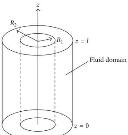
This equation indicates a relationship between the dynamic fluid viscosity𝜂, density of the fluid 𝜌, and the elastic constants. The roots of (41) give the infinite natural frequen-cies𝜔. R2 R1 z z = l Fluid domain z = 0
Figure 1: Configuration of the viscous oscillations of a cylindrical incompressible fluid of length𝑙 in circular cylindrical coordinate system(𝑟, 𝜃, 𝑧). 𝑅1 and𝑅2are the inner and outer radius of fluid domain, respectively.
R2
Fluid domain
R1
Figure 2: Geometry of fluid domain.
5. Analytical, Numerical
Results and Validation
Numerical calculations were performed on the example of the hollow cylinder (Figures1,2, and3) with𝑙 = 0.15 [m], and different dimensions such as the inner radius𝑅1 = 0.07 [m] and the outer radius𝑅2= 0.09 [m] of fluid domain are used. The fluid used in the hollow cylinder for which density of 920 [kg⋅m−3] and dynamic’s viscosity of 0.1 [Pa⋅s] is assumed.
The following values of parameters of the the elastic solid are in contact with a viscous liquid were assumed: 𝜌𝑠 = 1150 [kg/m3],]𝑠= 0.48, 𝐸 = 3 ⋅ 105[Pa], and the inner radius of elastic solid𝑅0= 0.068 [m].
With the derived eigenfrequency equations, natural fre-quencies𝜔𝑛𝑚 = Im(]𝛼2𝑛𝑚𝑗) for each pair of (𝑛, 𝑚) are cal-culated in the software Mathematica.𝑚 and 𝑛 denote the mode in axial and azimuthal (propagating clockwise around the vortex) direction, respectively. To validate the analytical results, the natural frequencies and mode shapes are also computed using Comsol Multiphysics FEM Simulation Soft-ware. The natural frequencies are computed directly from
R2
Fluid domain
Solid domain R1
R0
Figure 3: Geometry of fluid-solid interation model.𝑅0and𝑅1are the inner and outer radius of solid domain, respectively.
1 2 3 4 5 6 7 0 1 2 3 4 5 6 Axial wavenumber m No-slip-no-slip No-slip-normal stress-free
Normal stress-free-normal stress-free 𝜔
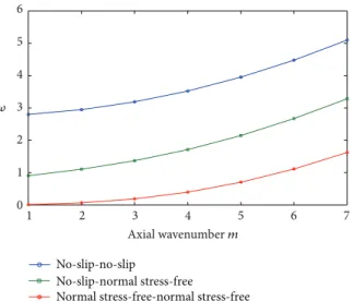
Figure 4: Variations of flexural eigenmode for different boundary conditions. 1 2 3 4 5 6 7 0 1 2 3 4 5 6 No-slip-no-slip No-slip-normal stress-free
Normal stress-free-normal stress-free 𝜔
Axial wavenumber m
Figure 5: Variations of breathing eigenmode for different boundary conditions. 1 2 3 4 5 6 7 0 1 2 3 4 5 6 No-slip-no-slip No-slip-normal stress-free
Normal stress-free-normal stress-free 𝜔
Axial wavenumber m
Figure 6: Variations of torsional eigenmode for different boundary conditions.
Table 1: Natural frequencies𝜔 [rd/s] for various mode shapes in the case of “no-slip-no-slip” boundary conditions.
No. (𝑛, 𝑚) Present FEM Mode shape 1 (0, 0) 2.694 2.694 Torsional 2 (0, 1) 2.742 2.742 Torsional 3 (1, 1) 2.755 2.755 Flexural 4 (2, 1) 2.800 2.800 Breathing 5 (3, 1) 2.882 2.882 Breathing 6 (0, 2) 2.885 2.885 Torsional 7 (1, 2) 2.900 2.900 Flexural 8 (2, 2) 2.948 2.948 Breathing 9 (4, 1) 3.000 3.000 Breathing 10 (3, 2) 3.030 3.030 Breathing 11 (0, 3) 3.124 3.124 Torsional 12 (1, 3) 3.140 3.140 Flexural 13 (4, 2) 3.147 3.147 Breathing 14 (5, 1) 3.153 3.153 Breathing 15 (2, 3) 3.189 3.189 Breathing 16 (3, 3) 3.271 3.271 Breathing 17 (5, 2) 3.299 3.299 Breathing 18 (6, 1) 3.341 3.341 Breathing
(24) for torsion vibration. For longitudinal vibration, (28) can be used to determine the corresponding natural frequencies. Tables 1 and 2 show the comparison of the first 18 natural frequencies and the corresponding mode shapes of viscous fluid by FEM and the present method (see (16) and (20)). For example in the case of “no-slip-normal stress-free” boundary conditions, in the first 18 natural frequencies, four correspond to flexural vibration (𝑛 = 1), nine to breathing vibration (𝑛 ⩾ 2), four to torsional vibration, and one to longitudinal vibration. The very good agreement is observed between the results of the present method and those of FEM and the relative difference ((FEM-Present)/Present) is ⩽1%. This shows that the algorithm implemented in Comsol
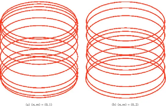
(a) (𝑛, 𝑚) = (0, 1) (b)(𝑛, 𝑚) = (0, 2)
Figure 7: The torsional modal shapes of(𝑛, 𝑚): streamlines of components of velocity field.
(a) (𝑛, 𝑚) = (1, 1) (b)(𝑛, 𝑚) = (1, 2)
Figure 8: The flexural modal shapes of(1, 𝑚): streamlines of components of velocity field.
Multiphysics [26,27] software for numerical computation is highly reliable and accurate. This algorithm is based on the UMFPACK method [28]. Is the attention to use the numerical formulation in future for more general geometries.
Tables1and2and Figures4,5, and6show that natural frequencies are very sensitive to the nature of the boundary conditions. It is seen that the effect of the free surface is very interesting and decrease the frequency of a fluid confined in a rigid cylinder.
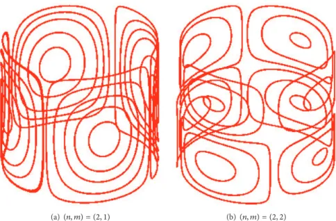
Figures 7, 8, and 9 show, respectively, the two modal shapes of the torsional, flexural, and breathing vibrations. The modal shape can be regarded as the mode(𝑛, 𝑚), where 𝑛 is
the modal number in the circumferential direction and𝑚 is the modal number in the axial direction. The modal shapes are not in order with the parameters𝑛 and 𝑚. This feature of cylindrical vibration is different from that of beam vibration in which the order increases with the modal parameter. Therefore in the vibration of the cylinder, one should be careful to find the right mode of the vibration.
In this paper, the effects of boundary conditions and of cylindrical parameters on the natural frequencies of cylindri-cal viscous fluid are presented with the present method. In these studies, investigations are carried out to study the effects of circumferential mode𝑛, axial mode 𝑚, and fluid thickness
(a)(𝑛, 𝑚) = (2, 1) (b)(𝑛, 𝑚) = (2, 2)
Figure 9: The breathing modal shapes of(2, 𝑚): streamlines of components of velocity field.
1 2 3 4 5 6 7 8 9 10 11 12 13 14 15 16 2 4 6 8 10 12 Circumferential wavenumber n 𝜔 m = 0 m = 1 m = 2 m = 3 m = 4
Figure 10: Variations of the natural frequencies𝜔 for different values 𝑚 with the mode 𝑚 with the mode 𝑛.
𝑒 = 𝑅2− 𝑅1on the frequencies. Influence of viscosity on the
natural frequencies of an elastic solid is also investigated. First, one investigates how the natural frequencies vary with the axial mode 𝑚. Figure 10 shows that the natural frequencies increase as the axial mode𝑚 increases except when𝑚 = 0. This value of 𝑚 corresponds to 2D problem of viscous oscillations.
Secondly, one investigates how the frequencies vary with the fluid thickness. Figures11,12, and13show that the fluid thickness has a strong influence on the natural frequencies.
Thirdly, one investigates how the dense fluid (added mass) affects the natural frequencies. Tables3and 4 show the coupled and uncoupled natural frequencies varying with circumferential and axial mode (𝑛, 𝑚). As 𝑛 increases, the
1 2 3 4 5 6 7 8 9 10 0 10 20 30 40 50 Axial wavenumber m e = 0.02 e = 0.015 e = 0.01e = 0.005 𝜔
Figure 11: Variations of the torsional eigenmode (𝑛 = 0) 𝜔 for different fluid’s thickness𝑒 with the mode 𝑚.
difference between the coupled and uncoupled natural fre-quencies increases. Figures14and15show that the presence of fluid has no influence on the modal shapes of an elastic solid.
6. Conclusion
We have presented an analytic solution for the Stokes eigen-modes of a viscous incompressible cylindrical fluid. Using the Helmholtz decomposition for the velocity field, we obtain an eigenvalue problem for 𝜔. The analytical results are in very good agreement with FEM results. This analytic method clearly distinguishes between the potential and rotational components and the contributions of each to various flow variables can be analyzed if one wishes so. The present solution is for cylindrical viscous fluid and is not limited to
1 2 3 4 5 6 7 8 9 10 0 10 20 30 40 50 Axial wavenumber m e = 0.02 e = 0.015 e = 0.01e = 0.005 𝜔
Figure 12: Variations of the flexural eigenmode (𝑛 = 1) 𝜔 for different fluid’s thickness𝑒 with the mode 𝑚.
1 2 3 4 5 6 7 8 9 10 0 8 16 24 32 40 Axial wavenumber m e = 0.02 e = 0.015 e = 0.01e = 0.005 𝜔
Figure 13: Variations of the breathing eigenmode (𝑛 = 2) 𝜔 for different fluid’s thickness𝑒 with the mode 𝑚.
a cylindrical shape. The same scalar potentials can be used to obtain stokes eigenmodes in the case of a spherical geometry. Finally, a knowledge of the stokes eigenmodes of viscous fluid is likely to be of use in performing a dynamic analysis by modal projection method.
Appendices
A.
The matrixM1in (16) is defined as follows:
M1= [ [ [ [ [ [ [ [ 𝑎11 𝑎12 𝑎13 𝑎14 𝑎15 𝑎16 𝑎21 𝑎22 𝑎23 𝑎24 𝑎25 𝑎26 𝑎31 𝑎32 0 0 𝑎35 𝑎36 𝑎41 𝑎42 𝑎43 𝑎44 𝑎45 𝑎46 𝑎51 𝑎52 𝑎53 𝑎54 𝑎55 𝑎56 𝑎61 𝑎62 0 0 𝑎65 𝑎66 ] ] ] ] ] ] ] ] , (A.1)
Table 2: Natural nfrequencies𝜔 [rd/s] for various mode shapes in the case of “no-slip-normal stress-free” boundary conditions.
No. (𝑛, 𝑚) Present FEM Mode shape 1 (1, 1) 0.889 0.889 Flexural 2 (0, 0) 0.898 0.898 Torsional 3 (2, 1) 0.908 0.908 Breathing 4 (0, 1) 0.946 0.946 Torsional 5 (0, 1) 0.951 0.951 Longitudinal 6 (3, 1) 0.984 0.984 Breathing 7 (1, 0) 0.990 0.990 Flexural 8 (1, 2) 1.087 1.087 Flexural 9 (0, 2) 1.089 1.089 Torsional 10 (2, 2) 1.1070 1.1070 Breathing 11 (4, 1) 1.1073 1.1073 Breathing 12 (1, 1) 1.113 1.113 Flexural 13 (3, 2) 1.171 1.171 Breathing 14 (2, 0) 1.251 1.251 Breathing 15 (5, 1) 1.271 1.271 Breathing 16 (4, 2) 1.281 1.281 Breathing 17 (0, 3) 1.327 1.327 Torsional 18 (1, 3) 1.337 1.337 Flexural
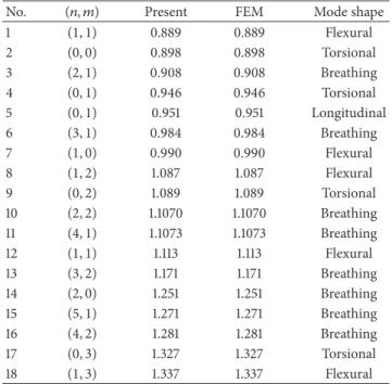
Table 3: Uncoupled natural frequencies𝜔 [rd/s] for various mode shapes of elastic solid.
No. (𝑛, 𝑚) Present FEM Mode shape 1 (2, 0) 0.952 0.952 Breathing 2 (3, 0) 2.693 2.693 Breathing 3 (4, 0) 5.157 5.157 Breathing 4 (4, 1) 7.145 7.145 Breathing 5 (3, 1) 7.389 7.389 Breathing 6 (5, 0) 8.326 8.326 Breathing 7 (5, 1) 9.431 9.431 Breathing 8 (2, 1) 11.456 11.456 Breathing 9 (6, 0) 12.190 12.190 Breathing 10 (6, 1) 13.035 13.035 Breathing 11 (5, 2) 14.379 14.379 Breathing 12 (4, 2) 14.700 14.700 Breathing 13 (6, 2) 16.504 16.504 Breathing 14 (7, 0) 16.739 16.739 Breathing 15 (7, 1) 17.500 17.500 Breathing 16 (3, 2) 18.005 18.005 Breathing 17 (7, 2) 20.270 20.270 Breathing 18 (1, 1) 20.289 20.289 Flexural where 𝑎11= 𝐼𝑛(𝑘𝑧𝑅1) , 𝑎12= 𝐾𝑛(𝑘𝑧𝑅1) , 𝑎13= −𝑅𝑛 1𝐽𝑛(𝑘𝜓𝑅1) ,
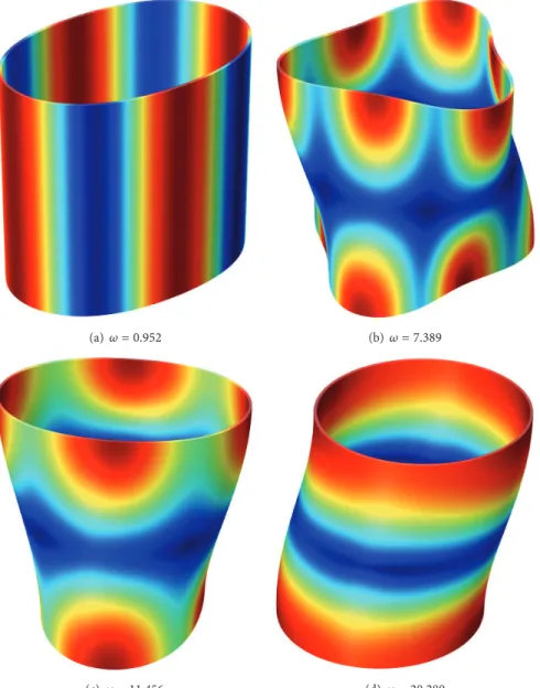
(a)𝜔 = 0.952 (b) 𝜔 = 7.389
(c)𝜔 = 11.456 (d) 𝜔 = 20.289
Figure 14: The modal shapes(𝑛, 𝑚) of elastic solid without fluid: the colours pertain to the displacement filed.
𝑎14= −𝑅𝑛 1𝑌𝑛(𝑘𝜓𝑅1) , 𝑎15= 𝑘𝑧𝐽𝑛(𝑘𝜓𝑅1) , 𝑎16= 𝑘𝑧𝑌𝑛(𝑘𝜓𝑅1) , 𝑎21= 𝑅𝑛 1𝐼𝑛(𝑘𝑧𝑅1) , 𝑎22= 𝑛 𝑅1𝐾𝑛(𝑘𝑧𝑅1) , 𝑎23= −𝐽𝑛(𝑘𝜓𝑅1) , 𝑎24= −𝑌𝑛(𝑘𝜓𝑅1) , 𝑎25= 𝑛𝑘𝑅𝑧 1𝐽𝑛(𝑘𝜓𝑅1) , 𝑎26= 𝑛𝑘𝑧 𝑅1 𝑌𝑛(𝑘𝜓𝑅1) , 𝑎31= −𝑘𝑧𝐼𝑛(𝑘𝑧𝑅1) , 𝑎32= −𝑘𝑧𝐾𝑛(𝑘𝑧𝑅1) , 𝑎35= 𝑘2𝜓𝐽𝑛(𝑘𝜓𝑅1) , 𝑎36= 𝑘2𝜓𝑌𝑛(𝑘𝜓𝑅1) , 𝑎41= 𝐼𝑛(𝑘𝑧𝑅2) , 𝑎42= 𝐾𝑛(𝑘𝑧𝑅2) , 𝑎43= −𝑅𝑛 2𝐽𝑛(𝑘𝜓𝑅2) , 𝑎44= −𝑅𝑛 2𝑌𝑛(𝑘𝜓𝑅2) , 𝑎45= 𝑘𝑧𝐽𝑛(𝑘𝜓𝑅2) , 𝑎46= 𝑘𝑧𝑌𝑛(𝑘𝜓𝑅2) , 𝑎51= 𝑅𝑛 2𝐼𝑛(𝑘𝑧𝑅2) , 𝑎52= 𝑛 𝑅2𝐾𝑛(𝑘𝑧𝑅2) , 𝑎53= −𝐽𝑛(𝑘𝜓𝑅2) , 𝑎54= −𝑌𝑛(𝑘𝜓𝑅2) , 𝑎55=𝑛𝑘𝑅𝑧 2 𝐽𝑛(𝑘𝜓𝑅2) , 𝑎56= 𝑛𝑘𝑧 𝑅2𝑌𝑛(𝑘𝜓𝑅2) ,
Table 4: Coupled natural nfrequencies𝜔 [rd/s] for various mode shapes.
No. (𝑛, 𝑚) Present FEM Mode shape 1 (0, 1) 0.535 0.535 Torsional 2 (1, 1) 0.566 0.566 Flexural 3 (2, 1) 0.645 0.645 Breathing 4 (0, 2) 0.678 7.145 Torsional 5 (1, 2) 0.699 0.699 Flexural 6 (2, 0) 0.702 0.702 Breathing 7 (3, 1) 0.749 0.749 Breathing 8 (2, 2) 0.760 0.760 Breathing 9 (0, 1) 0.780 0.780 Longitudinal 10 (1, 1) 0.813 0.813 Flexural 11 (3, 2) 0.854 0.854 Breathing 12 (4, 1) 0.872 0.872 Breathing 13 (0, 3) 0.917 0.917 Torsional 14 (3, 0) 0.924 0.924 Breathing 15 (1, 3) 0.935 0.935 Flexural 16 (4, 2) 0.978 0.978 Breathing 17 (2, 3) 0.988 0.988 Breathing 18 (5, 1) 1.019 1.019 Breathing 𝑎61= −𝑘𝑧𝐼𝑛(𝑘𝑧𝑅2) , 𝑎62= −𝑘𝑧𝐾𝑛(𝑘𝑧𝑅2) , 𝑎65= 𝑘2𝜓𝐽𝑛(𝑘𝜓𝑅2) , 𝑎66= 𝑘2𝜓𝑌𝑛(𝑘𝜓𝑅2) . (A.2)
B.
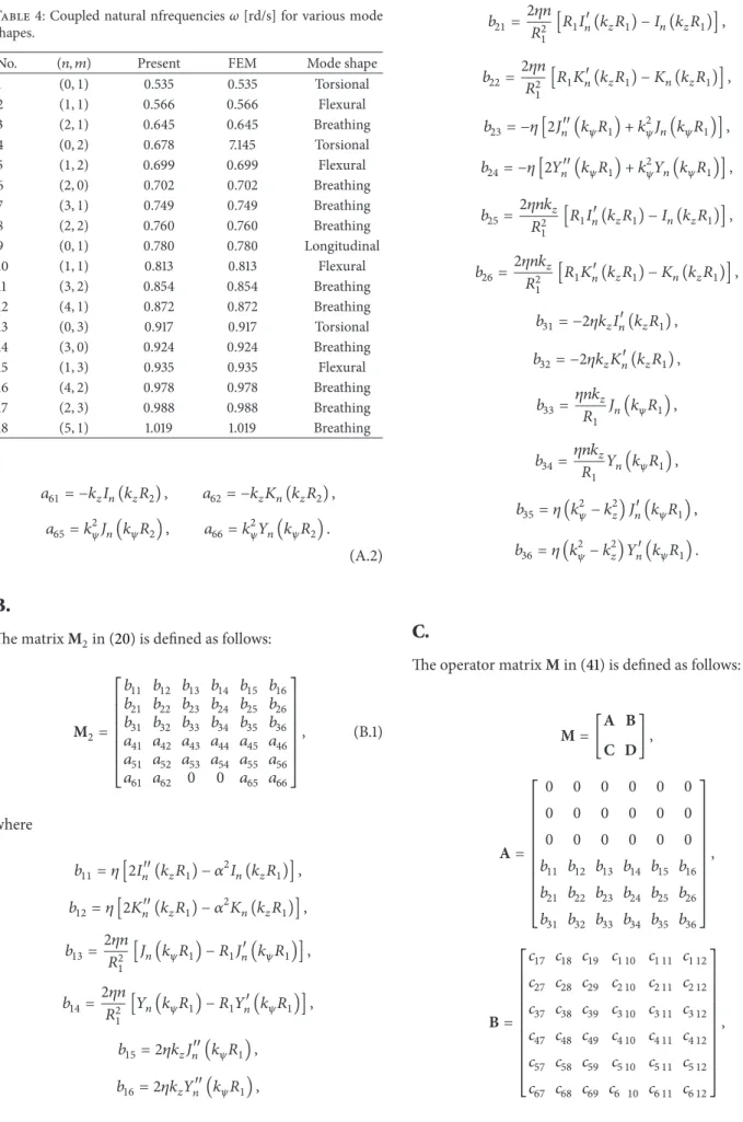
The matrixM2in (20) is defined as follows:
M2= [ [ [ [ [ [ [ [ 𝑏11 𝑏12 𝑏13 𝑏14 𝑏15 𝑏16 𝑏21 𝑏22 𝑏23 𝑏24 𝑏25 𝑏26 𝑏31 𝑏32 𝑏33 𝑏34 𝑏35 𝑏36 𝑎41 𝑎42 𝑎43 𝑎44 𝑎45 𝑎46 𝑎51 𝑎52 𝑎53 𝑎54 𝑎55 𝑎56 𝑎61 𝑎62 0 0 𝑎65 𝑎66 ] ] ] ] ] ] ] ] , (B.1) where 𝑏11= 𝜂 [2𝐼𝑛(𝑘𝑧𝑅1) − 𝛼2𝐼𝑛(𝑘𝑧𝑅1)] , 𝑏12= 𝜂 [2𝐾𝑛(𝑘𝑧𝑅1) − 𝛼2𝐾𝑛(𝑘𝑧𝑅1)] , 𝑏13= 2𝜂𝑛𝑅2 1 [𝐽𝑛(𝑘𝜓𝑅1) − 𝑅1𝐽 𝑛(𝑘𝜓𝑅1)] , 𝑏14=2𝜂𝑛𝑅2 1 [𝑌𝑛(𝑘𝜓𝑅1) − 𝑅1𝑌 𝑛(𝑘𝜓𝑅1)] , 𝑏15= 2𝜂𝑘𝑧𝐽𝑛(𝑘𝜓𝑅1) , 𝑏16= 2𝜂𝑘𝑧𝑌𝑛(𝑘𝜓𝑅1) , 𝑏21= 2𝜂𝑛𝑅2 1 [𝑅1𝐼 𝑛(𝑘𝑧𝑅1) − 𝐼𝑛(𝑘𝑧𝑅1)] , 𝑏22= 2𝜂𝑛𝑅2 1 [𝑅1𝐾 𝑛(𝑘𝑧𝑅1) − 𝐾𝑛(𝑘𝑧𝑅1)] , 𝑏23= −𝜂 [2𝐽𝑛(𝑘𝜓𝑅1) + 𝑘2𝜓𝐽𝑛(𝑘𝜓𝑅1)] , 𝑏24= −𝜂 [2𝑌𝑛(𝑘𝜓𝑅1) + 𝑘2𝜓𝑌𝑛(𝑘𝜓𝑅1)] , 𝑏25=2𝜂𝑛𝑘𝑅2𝑧 1 [𝑅1𝐼 𝑛(𝑘𝑧𝑅1) − 𝐼𝑛(𝑘𝑧𝑅1)] , 𝑏26=2𝜂𝑛𝑘𝑅2𝑧 1 [𝑅1𝐾 𝑛(𝑘𝑧𝑅1) − 𝐾𝑛(𝑘𝑧𝑅1)] , 𝑏31= −2𝜂𝑘𝑧𝐼𝑛(𝑘𝑧𝑅1) , 𝑏32= −2𝜂𝑘𝑧𝐾𝑛(𝑘𝑧𝑅1) , 𝑏33=𝜂𝑛𝑘𝑅 𝑧 1 𝐽𝑛(𝑘𝜓𝑅1) , 𝑏34=𝜂𝑛𝑘𝑅 𝑧 1 𝑌𝑛(𝑘𝜓𝑅1) , 𝑏35= 𝜂 ( 𝑘2𝜓− 𝑘2𝑧) 𝐽𝑛(𝑘𝜓𝑅1) , 𝑏36= 𝜂 ( 𝑘𝜓2− 𝑘2𝑧) 𝑌𝑛(𝑘𝜓𝑅1) . (B.2)
C.
The operator matrixM in (41) is defined as follows:
M = [A B C D] , A = [ [ [ [ [ [ [ [ [ [ [ [ 0 0 0 0 0 0 0 0 0 0 0 0 0 0 0 0 0 0 𝑏11 𝑏12 𝑏13 𝑏14 𝑏15 𝑏16 𝑏21 𝑏22 𝑏23 𝑏24 𝑏25 𝑏26 𝑏31 𝑏32 𝑏33 𝑏34 𝑏35 𝑏36 ] ] ] ] ] ] ] ] ] ] ] ] , B = [ [ [ [ [ [ [ [ [ [ [ [ 𝑐17 𝑐18 𝑐19 𝑐1 10 𝑐1 11 𝑐1 12 𝑐27 𝑐28 𝑐29 𝑐2 10 𝑐2 11 𝑐2 12 𝑐37 𝑐38 𝑐39 𝑐3 10 𝑐3 11 𝑐3 12 𝑐47 𝑐48 𝑐49 𝑐4 10 𝑐4 11 𝑐4 12 𝑐57 𝑐58 𝑐59 𝑐5 10 𝑐5 11 𝑐5 12 𝑐67 𝑐68 𝑐69 𝑐6 10 𝑐6 11 𝑐6 12 ] ] ] ] ] ] ] ] ] ] ] ] ,
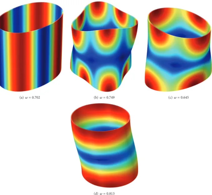
(a) 𝜔 = 0.702 (b) 𝜔 = 0.749 (c)𝜔 = 0.645
(d) 𝜔 = 0.813
Figure 15: The modal shapes(𝑛, 𝑚) of elastic solid with fluid: the colours pertain to the displacement filed.
C = [ [ [ [ [ [ [ [ 𝑎11 𝑎12 𝑎13 𝑎14 𝑎15 𝑎16 𝑎21 𝑎22 𝑎23 𝑎24 𝑎25 𝑎26 𝑎31 𝑎32 0 0 𝑎35 𝑎36 𝑐10 1 𝑐10 2 𝑐10 3 𝑐10 4 𝑐10 5 𝑐10 6 𝑐11 1 𝑐11 2 𝑐11 3 𝑐11 4 𝑐11 5 𝑐11 6 𝑐12 1 𝑐12 2 𝑐12 3 𝑐12 4 𝑐12 5 𝑐12 6 ] ] ] ] ] ] ] ] , D = [ [ [ [ [ [ [ [ 𝑐77 𝑐78 𝑐79 𝑐7 10 𝑐7 11 𝑐7 12 𝑐87 𝑐88 𝑐89 𝑐8 10 𝑐8 11 𝑐8 12 𝑐97 𝑐98 0 0 𝑐9 11 𝑐9 12 0 0 0 0 0 0 0 0 0 0 0 0 0 0 0 0 0 0 ] ] ] ] ] ] ] ] , (C.1) where 𝑐17= 2𝜇 [𝐼𝑛(𝑘Φ𝑅0) + 𝜆]2 𝑓𝛼4 2𝜇𝑐2 𝐿 𝐼𝑛(𝑘Φ𝑅0)] , 𝑐18= 2𝜇 [𝐾𝑛 (𝑘Φ𝑅0) + 𝜆]2 𝑓𝛼4 2𝜇𝑐2 𝐿 𝐾𝑛(𝑘Φ𝑅0)] , 𝑐19= 2𝜇𝑛𝑅2 0 [𝐼𝑛(𝑘Ψ𝑅0) − 𝑅0𝐼 𝑛(𝑘Ψ𝑅0)] , 𝑐1 10=2𝜇𝑛𝑅2 0 [𝐾𝑛(𝑘Ψ𝑅0) − 𝑅0𝐾 𝑛(𝑘Ψ𝑅0)] ,
𝑐1 11= 2𝜇𝑘𝑧𝐼𝑛(𝑘Ψ𝑅0) , 𝑐1 12= 2𝜇𝑘𝑧𝐾𝑛 (𝑘Ψ𝑅0) , 𝑐27= 2𝜇𝑛𝑅2 0 [𝑅0𝐼𝑛(𝑘Φ𝑅0) − 𝐼𝑛(𝑘Φ𝑅0)] , 𝑐28= 2𝜇𝑛𝑅2 0 [𝑅0𝐾 𝑛(𝑘Φ𝑅0) − 𝐾𝑛(𝑘Φ𝑅0)] , 𝑐29= 𝜇 [𝑘2Ψ𝐼𝑛(𝑘Ψ𝑅0) − 2𝐼𝑛(𝑘Ψ𝑅0)] , 𝑐2 10= 𝜇 [𝑘2Ψ𝐾𝑛(𝑘Ψ𝑅0) − 2𝐾𝑛(𝑘Ψ𝑅0)] , 𝑐2 11= 2𝜇𝑛𝑘𝑅2𝑧 0 [𝑅0𝐼𝑛(𝑘Ψ𝑅0) − 𝐼𝑛(𝑘Ψ𝑅0)] , 𝑐2 12= 2𝜇𝑛𝑘𝑅2𝑧 0 [𝑅0𝐾 𝑛(𝑘Ψ𝑅0) − 𝐾𝑛(𝑘Ψ𝑅0)] , 𝑐37= −2𝜇𝑘𝑧𝐼𝑛(𝑘Φ𝑅0) , 𝑐38= −2𝜇𝑘𝑧𝐾𝑛(𝑘Φ𝑅0) , 𝑐39= 𝜇𝑛𝑘𝑅 𝑧 0 𝐼 𝑛(𝑘Ψ𝑅0) , 𝑐3 10= 𝜇𝑛𝑘𝑅 𝑧 0 𝐾 𝑛(𝑘Ψ𝑅0) , 𝑐3 11= −𝜇 ( 𝑘2Ψ+ 𝑘2𝑧) 𝐼𝑛(𝑘Ψ𝑅0) , 𝑐3 12= −𝜇 ( 𝑘2Ψ+ 𝑘2𝑧) 𝐾𝑛(𝑘Ψ𝑅0) , 𝑐47= 2𝜇 [𝐼𝑛(𝑘Φ𝑅1) + 𝜆]2 𝑓𝛼4 2𝜇𝑐2 𝐿 𝐼𝑛(𝑘Φ𝑅1)] , 𝑐48= 2𝜇 [𝐾𝑛(𝑘Φ𝑅1) + 𝜆]2 𝑓𝛼4 2𝜇𝑐2 𝐿 𝐾𝑛(𝑘Φ𝑅1)] , 𝑐49=2𝜇𝑛𝑅2 1 [𝐼𝑛(𝑘Ψ𝑅1) − 𝑅1𝐼 𝑛(𝑘Ψ𝑅1)] , 𝑐4 10= 2𝜇𝑛𝑅2 1 [𝐾𝑛(𝑘Ψ𝑅1) − 𝑅1𝐾 𝑛(𝑘Ψ𝑅1)] , 𝑐4 11= 2𝜇𝑘𝑧𝐼𝑛(𝑘Ψ𝑅1) , 𝑐4 12= 2𝜇𝑘𝑧𝐾𝑛 (𝑘Ψ𝑅1) , 𝑐57= 2𝜇𝑛𝑅2 1 [𝑅1𝐼 𝑛(𝑘Φ𝑅1) − 𝐼𝑛(𝑘Φ𝑅1)] , 𝑐58= 2𝜇𝑛𝑅2 1 [𝑅1𝐾 𝑛(𝑘Φ𝑅1) − 𝐾𝑛(𝑘Φ𝑅1)] , 𝑐59= 𝜇 [𝑘2Ψ𝐼𝑛(𝑘Ψ𝑅1) − 2𝐼𝑛(𝑘Ψ𝑅1)] , 𝑐5 10= 𝜇 [𝑘2Ψ𝐾𝑛(𝑘Ψ𝑅1) − 2𝐾𝑛(𝑘Ψ𝑅1)] , 𝑐5 11= 2𝜇𝑛𝑘𝑅2 𝑧 1 [𝑅1𝐼 𝑛(𝑘Ψ𝑅1) − 𝐼𝑛(𝑘Ψ𝑅1)] , 𝑐5 12=2𝜇𝑛𝑘𝑅2 𝑧 1 [𝑅1𝐾 𝑛(𝑘Ψ𝑅1) − 𝐾𝑛(𝑘Ψ𝑅1)] , 𝑐67= −2𝜇𝑘𝑧𝐼𝑛(𝑘Φ𝑅1) , 𝑐68= −2𝜇𝑘𝑧𝐾𝑛(𝑘Φ𝑅1) , 𝑐69=𝜇𝑛𝑘𝑅 𝑧 1 𝐼 𝑛(𝑘Ψ𝑅1) , 𝑐6 10= 𝜇𝑛𝑘𝑅 𝑧 1 𝐾 𝑛(𝑘Ψ𝑅1) , 𝑐6 11= −𝜇 ( 𝑘2Ψ+ 𝑘2𝑧) 𝐼𝑛(𝑘Ψ𝑅1) , 𝑐6 12= −𝜇 ( 𝑘2Ψ+ 𝑘2𝑧) 𝐾𝑛(𝑘Ψ𝑅1) , 𝑐77= ]𝛼2𝐼𝑛(𝑘Φ𝑅1) , 𝑐78= ]𝛼2𝐾𝑛(𝑘Φ𝑅1) , 𝑐79= −]𝛼 2𝑛 𝑅1 𝐼 𝑛(𝑘Ψ𝑅1) , 𝑐7 10= −]𝛼 2𝑛 𝑅1 𝐾 𝑛(𝑘Ψ𝑅1) , 𝑐7 11= ]𝛼2𝑘𝑧𝐼𝑛(𝑘Ψ𝑅1) , 𝑐7 12= ]𝛼2𝑘𝑧𝐾𝑛(𝑘Ψ𝑅1) , 𝑐87= ]𝛼2𝑅𝑛 1𝐼𝑛(𝑘Φ𝑅1) , 𝑐88= ]𝛼2𝑅𝑛 1𝐾𝑛(𝑘Φ𝑅1) , 𝑐89= −]𝛼2𝐼𝑛(𝑘Ψ𝑅1) , 𝑐8 10= −]𝛼2𝐾𝑛(𝑘Ψ𝑅1) , 𝑐8 11= ]𝛼2𝑛𝑘𝑅𝑧 1 𝐼𝑛(𝑘Ψ𝑅1) , 𝑐8 12= ]𝛼2𝑛𝑘𝑅𝑧 1𝐾𝑛(𝑘Ψ𝑅1) , 𝑐97= −]𝛼2𝑘𝑧𝐼𝑛(𝑘Φ𝑅1) , 𝑐98= −]𝛼2𝑘𝑧𝐾𝑛(𝑘Φ𝑅1) , 𝑐9 11= −]𝛼2𝑘2Ψ𝐼𝑛(𝑘Ψ𝑅1) , 𝑐9 12= −]𝛼2𝑘2Ψ𝐾𝑛(𝑘Ψ𝑅1) , 𝑐10 1= 𝜂 [2𝐼𝑛(𝑘𝑧𝑅2) − 𝛼2𝐼𝑛(𝑘𝑧𝑅2)] , 𝑐10 2= 𝜂 [2𝐾𝑛(𝑘𝑧𝑅2) − 𝛼2𝐾𝑛(𝑘𝑧𝑅2)] ,
𝛼 200 150
100 50
First order value 𝛼 = 159.205 det[M1] for (n, m) = (1, 1)
Figure 16: Analytical calculation of eigenvalues𝛼.
𝑐10 3= 2𝜂𝑅𝑛2 2[𝐽𝑛(𝑘𝜓𝑅2) − 𝑅2𝐽 𝑛(𝑘𝜓𝑅2)] , 𝑐10 4= 2𝜂𝑅𝑛2 2[𝑌𝑛(𝑘𝜓𝑅2) − 𝑅2𝑌 𝑛(𝑘𝜓𝑅2)] , 𝑐10 5= 2𝜂𝑘𝑧𝐽𝑛(𝑘𝜓𝑅2) , 𝑐10 6= 2𝜂𝑘𝑧𝑌𝑛(𝑘𝜓𝑅2) , 𝑐11 1= 2𝜂𝑅𝑛2 2 [𝑅2𝐼𝑛(𝑘𝑧𝑅2) − 𝐼𝑛(𝑘𝑧𝑅2)] , 𝑐11 2= 2𝜂𝑅𝑛2 2[𝑅2𝐾 𝑛(𝑘𝑧𝑅2) − 𝐾𝑛(𝑘𝑧𝑅2)] , 𝑐11 3= −𝜂 [2𝐽𝑛(𝑘𝜓𝑅2) + 𝑘2𝜓𝐽𝑛(𝑘𝜓𝑅2)] , 𝑐11 4= −𝜂 [2𝑌𝑛(𝑘𝜓𝑅2) + 𝑘2𝜓𝑌𝑛(𝑘𝜓𝑅2)] , 𝑐11 5= 2𝜂𝑛𝑘𝑅2𝑧 2 [𝑅2𝐼 𝑛(𝑘𝑧𝑅2) − 𝐼𝑛(𝑘𝑧𝑅2)] , 𝑐11 6= 2𝜂𝑛𝑘𝑅2𝑧 2 [𝑅2𝐾 𝑛(𝑘𝑧𝑅2) − 𝐾𝑛(𝑘𝑧𝑅2)] , 𝑐12 1= −2𝜂𝑘𝑧𝐼𝑛(𝑘𝑧𝑅2) , 𝑐12 2= −2𝜂𝑘𝑧𝐾𝑛(𝑘𝑧𝑅2) , 𝑐12 3= 𝜂𝑛𝑘𝑅𝑧 2 𝐽𝑛(𝑘𝜓𝑅2) , 𝑐12 4= 𝜂𝑛𝑘𝑅𝑧 2 𝑌𝑛(𝑘𝜓𝑅2) , 𝑐12 5= 𝜂 ( 𝑘2𝜓− 𝑘𝑧2) 𝐽𝑛(𝑘𝜓𝑅2) , 𝑐12 6= 𝜂 ( 𝑘2𝜓− 𝑘2𝑧) 𝑌𝑛(𝑘𝜓𝑅2) . (C.2)
D.
SeeFigure 16.References
[1] F. Razafimahery, “Ecoulements externes de Stokes dans des domaines non r´eguliers et condition de Kutta-Joukowski g´en´eralis´ee,” Zeitschrift f¨ur Angewandte Mathematik und Physik, vol. 54, pp. 125–148, 2003.
[2] H. Bruus, Theoretical Microfluidics, Oxford University Press, New York, NY, USA, 2008.
[3] G. Karniadakis, A. Beskok, and N. Aluru, Microflows and
Nano-flows: Fundamentals and Simulation, Springer, 2005.
[4] S. Childress, Mechanics of Swimming and Flying, Cambridge University Press, 1981.
[5] A. S. Ashour, “Propagation of guided waves in a fluid layer bounded by two viscoelastic transversely isotropic solids,”
Journal of Applied Geophysics, vol. 44, no. 4, pp. 327–336, 2000.
[6] A. S. Ashour, “Wave motion in a viscous fluid-filled fracture,”
International Journal of Engineering Science, vol. 38, no. 5, pp.
505–515, 2000.
[7] I. Edelman, “On the existence of the low-frequency surface waves in a porous medium,” Comptes Rendus, vol. 332, no. 1, pp. 43–49, 2004.
[8] W. Seemann and J. Wauer, “Fluid-structural coupling of vibrat-ing bodies in a surroundvibrat-ing confined liquid,” Zeitschrift fur
Angewandte Mathematik und Mechanik, vol. 76, no. 2, pp. 67–79,
1996.
[9] S. G. Kadyrov, J. Wauer, and S. V. Sorokin, “A potential technique in the theory of interaction between a structure and a viscous, compressible fluid,” Archive of Applied Mechanics, vol. 71, no. 6-7, pp. 405–416-7, 2001.
[10] E. Leriche and G. Labrosse, “Vector potential-vorticity relation-ship for the Stokes flows: application to the Stokes eigenmodes in 2D/3D closed domain,” Theoretical and Computational Fluid
Dynamics, vol. 21, no. 1, pp. 1–13, 2007.
[11] R. Rodr´ıguez and J. E. Solomin, “The order of convergence of eigenfrequencies in finite element approximations of fluid-structure interaction problems,” Mathematics of Computation, vol. 65, no. 216, pp. 1463–1475, 1996.
[12] A. Berm´udez and R. Rodr´ıguez, “Modelling an numerical solution of elastoacoustic vibrations with interface damping,”
International Journal for Numerical Methods in Engineering, vol.
46, no. 10, pp. 1763–1779, 1999.
[13] G. G. Stokes, “On the effect of the internal friction of fluids on the motion of pendulums,” Transactions of the Cambridge
Philo-sophical Society, vol. 9, pp. 8–106, 1851.
[14] H. Lamb, Hydrodynamics, Cambridge University Press, 1932. [15] D. D. Joseph, “Potential flow of viscous fluids: historical notes,”
International Journal of Multiphase Flow, vol. 32, no. 3, pp. 285–
310, 2006.
[16] R. Kidambi, “Oscillatory stokes flow in a cylindrical container,”
Fluid Dynamics Research, vol. 38, no. 4, pp. 274–294, 2006.
[17] P. N. Shankar, “Three-dimensional eddy structure in a cylindri-cal container,” Journal of Fluid Mechanics, vol. 342, pp. 97–118, 1997.
[18] G. Pontrelli and A. Tatone, “Wave propagation in a fluid flowing through a curved thin-walled elastic tube,” Journal of
FluidMechanics, vol. 5, pp. 113–133, 1971.
[19] B. Sweetman, M. Xenos, L. Zitella, and A. A. Linninger, “Three-dimensional computational prediction of cerebrospinal fluid flow in the human brain,” Computers in Biology and Medicine, vol. 41, no. 2, pp. 67–75, 2011.
[20] S. Gupta, M. Soellinger, P. Boesiger, D. Poulikakos, and V. Kurtcuoglu, “Three-dimensional computational modeling of subject-specific cerebrospinal fluid flow in the subarachnoid space,” Journal of Biomechanical Engineering, vol. 131, no. 2, 11 pages, 2009.
[21] V. V. Mokeyev, “On a method for vibration analysis of viscous compressible fluid-structure systems,” International Journal for
Numerical Methods in Engineering, vol. 59, no. 13, pp. 1703–1723,
2004.
[22] M. Morse and H. Feshbach, Methods of Theoretical Physics, McGraw-Hill, New York, NY, USA, 1946.
[23] R. Ohayon and C. Soize, Structural Acoustics and Vibration, Academic Press, 1997.
[24] M. P. Paidoussis, Fluid-Structure Interactions Slender Structures
and Axial Flow, vol. 1, London Academic Press, 1997.
[25] M. P. Paidoussis, Fluid-Structure Interactions Slender Structures
and Axial Flow, vol. 2, Elsevier Academic Press, London, UK,
2004.
[26] “Comsol Multiphysics 3.5a,” User’s Guide, 2008. [27] “Comsol Multiphysics 3.5a,” Reference Guide, 2008.
[28] T. A. Davis, “Algorithm 832: UMFPACK V4.3: an unsymmetric-pattern multifrontal method,” ACM Transactions on