Science Arts & Métiers (SAM)
is an open access repository that collects the work of Arts et Métiers Institute of
Technology researchers and makes it freely available over the web where possible.
This is an author-deposited version published in: https://sam.ensam.eu Handle ID: .http://hdl.handle.net/10985/8679
To cite this version :
Samuel PINSON, Laurent GUILLON - Sound speed profile characterization by the image source method - The Journal of the Acoustical Society of America - Vol. 128, n°4, p.1685-1693 - 2010
Any correspondence concerning this service should be sent to the repository Administrator : archiveouverte@ensam.eu
Sound speed profile characterization by the image source
method
S. Pinsona兲and L. Guillon
Institut de Recherche de l’Ecole Navale (IRENav), BCRM Brest, CC 600, F-29240 Brest Cedex 9, France 共Received 11 December 2009; revised 20 July 2010; accepted 30 July 2010兲
This paper presents the first results of an imaging technique that measures the geoacoustic structure of a seafloor in shallow water areas. The devices used were a broadband共100 Hz–6 kHz兲 acoustic source towed by a ship and a vertical array. Among all the acoustic paths existing in the water column, two are used: the direct one and the seabed-reflected one, the latter being composed of the reflections from the seafloor’s surface as well as that from each buried layer. Due to the good time resolution of the signal and to the short range configuration, the reflected signal can be modeled as a sum of contributions coming from image sources relative to the seabed layers. The seabed geometry and the sound speed profile can then be recovered with the detection and localization of these image sources. The map of the image sources is obtained by a function that combines back-propagation of signals and knowledge of the emitted pulse. The thickness and sound-speed of each layer is finally obtained by a position analysis of the image sources. The results obtained by this data-driven algorithm on both at-sea and synthetic data are satisfactory.
© 2010 Acoustical Society of America. 关DOI: 10.1121/1.3483720兴
PACS number共s兲: 43.30.Ma, 43.30.Pc, 43.60.Fg, 43.60.Rw 关NPC兴 Pages: 1685–1693
I. INTRODUCTION
Knowledge of seabed structure is essential to many ap-plications. Complementarily to direct geophysics measure-ments, remote sensing by acoustics has prove its ability to get both the geometry and the physical characteristics of the seabed. Most of the present-day techniques are based on an inversion process such as, for example, matched field methods1 or inversion of backscattering strength data.2 In 2000, C. Holland and J. Osler proposed a joint time-frequency method based on reflection coefficient measure-ment at short distance.3 In their measurements, they used a single hydrophone on a vertical array and a towed omnidi-rectional broadband source共Fig.1兲. This data was also used recently to study the dependence of the coherence on the nature of the seabed.4
Based on this geometrical configuration, an imaging method to invert the seafloor structure 共layering and sound speed profile兲 is presented in this paper. A classical imaging method used to image the seabed structure is the Kirchhoff migration5 which consists of backpropagating recorded sig-nals to geological interfaces共i.e., reflectors兲 that are equiva-lent in this case to extended sources. Here we consider these interfaces as acoustical mirrors on which images of the real source appear. The advantage of imaging the seafloor by searching for point sources is that it becomes possible to use high resolution array processing and then use the position of these image sources to determine the seabed structure with-out an inversion process. To that end, the full vertical array response with only one shot of the towed source is used.
The data used in this paper is presented on Section II. In Section III, the method with its hypothesis, its algorithm and
results on synthetic and real data are described. Finally, Sec-tion IV explains how the sound speed profile can be obtain from the image source locations.
II. DATA AND MODEL
The configuration of the experiment is a broadband source共100 Hz–6 kHz兲 20 cm bellow the sea surface and an array made of 15 hydrophones irregularly spaced over 64 m. The lowermost hydrophone is around 12 m above the seaf-loor共Fig.1兲. For modeled data, the configuration is the same as for experimental data.
The physical phenomenon that leads to recovery of the sound speed profile is the refraction of sound waves in the layers. Then, when the range between source and receivers is long, the refraction phenomenon is high. The range also needs to be short enough to avoid a total reflection phenom-enon on the interfaces which occurs at high incident angles. Here, with a 150 m water depth, the range between source and receivers for both real data and modeled data is 200 m, which is a good compromise. This distance leads to an inci-dent angle of 45° on the seafloor for the middle of the array which is far from the critical angle.
A. Synthetic data
Synthetic data is obtained by a numerical evaluation of the Sommerfeld integral, the exact analytical solution of the reflection of a spherical wave on layered media.6,7The trans-fer function Hnof this reflection between a source located at
r0s=共0,z0s兲 and a hydrophone n located at rn r =共rn r , zn r兲 is Hn共rn r ,r0s,兲 = ik
冕
0 /2−i⬁ J0共兩r0 s − rn r兩k sin兲R共 ,兲 ⫻ eik共zn r +z0s兲cossind, 共1兲a兲Author to whom correspondence should be addressed. Electronic mail:
where is the angle of incidence, the angular frequency, and k the wave number. The exponents s and r respectively stand for a source and a receiver. Because this integral is the result of plane wave decomposition, the term R共,兲 is the plane wave reflection coefficient and can be computed for an arbitrary layering of fluid or elastic media.8The time signal composed of the direct and the reflected wave at hydrophone n is sn共t兲 = FT−1
冋
冉
ei共共兩r0s−rn r 兩兲/c0兲 兩r0 s − rn r兩 + Hn共rn r ,r0s,兲冊
⫻ F共兲册
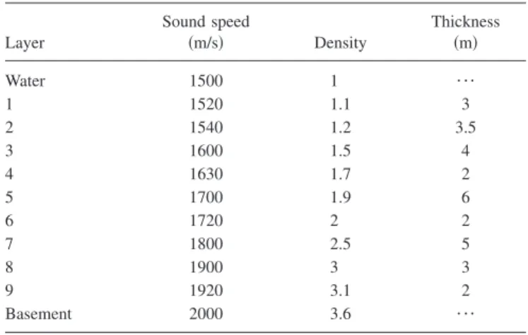
, 共2兲 where FT−1 is the inverse Fourier transform, F共兲 the emitted wavelet spectrum 共Fig. 2兲 and G0共r1, r2,兲=ei共共兩r1−r2兩兲/c0兲/兩r1− r2兩 the Green’s function of an homogeneous medium with a wave number k0=/c0, c0 being the sound speed in water. Note that the signal used for the synthetic data comes from the real data experiments共see Section II B兲. The choice of the geoacoustic structure for the synthetic data is driven by two opposite principles: on the one hand, it should be complex enough to prove the validity of the method, but on the other hand, it should be simple enough to avoid difficult interpretation. The simulated sea-bed is composed of 9 fluid sediment layers covering a semi-infinite fluid basement 共Table I兲. The synthetic data is then obtained with Eqs.共1兲and共2兲, R共,兲 being computed with these parameters.The temporal signal simulated for the 8thhydrophone of the array 共Fig. 3兲 shows visible echoes from the 10 inter-faces. Echoes from these interfaces are identified on Fig.3. Using Eqs. 共1兲 and 共2兲, multiple reflections between inter-faces are present in the computed signal but these echoes amplitudes are too small to be visible or to interfere with echoes from direct reflections.
B. Data from SCARAB experiment
The method developed here is also tested on real data acquired in June 1998 near Elba Island in Italy共Fig.4, left兲 as part of the SCARAB共Scattering And ReverberAtion from the sea Bottom兲 experiment series 共see Ref. 3 for details兲. The data used here are from site 2 where the water depth is 150 m and, from side-scan sonar data, the seabed is flat and featureless; bottom slopes are 0.3° or less. Geoacoustic in-version from broadband reflection data3shows sound speeds and densities consistent with a silty-clay sediment with inter-calating sandy sediments共Fig.4, right兲. One of the recorded signals is shown in Fig. 5. One can note the presence of a non-negligible additive noise but numerous seabed reflec-tions are nevertheless still visible.
FIG. 1. Sketch of the experiment. The source is 200 m away from the vertical array. The receiver array, moored on the seafloor, is made of 15 hydrophones, is 64 m long. The lowermost hydrophone is around 12 m above the seafloor.
FIG. 2. Signal emitted by the source共a兲 in the time domain and 共b兲 in the frequency domain.
TABLE I. Geoacoustic parameters for the synthetic data. The media used here are non-dissipative.
Layer Sound speed 共m/s兲 Density Thickness 共m兲 Water 1500 1 ¯ 1 1520 1.1 3 2 1540 1.2 3.5 3 1600 1.5 4 4 1630 1.7 2 5 1700 1.9 6 6 1720 2 2 7 1800 2.5 5 8 1900 3 3 9 1920 3.1 2 Basement 2000 3.6 ¯
FIG. 3. Temporal signal computed for the 8th hydrophone of the array.
Numbers 1–10 stand for interface reflections.
III. DETECTION OF IMAGE SOURCES A. Image sources
The image source method is widely used to simulate wave propagation. It models the reflected wave as a wave emitted by the image source located symmetrically behind the reflecting interface. This method is generally used for room acoustics,9propagation in a waveguide10,11or to model the reflection from a half space of an emission from a radar antenna.12 In these two last cases, the image source coordi-nates are complex in order to take into account the angular variations of the reflection coefficient.
This method based on the ray theory is usually used to model systems, but according to the author’s knowledge, not for performing a characterization. The ray theory is used in some geoacoustic inversion techniques13–15but two main dif-ferences exist with the image source method. First, in these works the geometric approximation is used to compute travel times or amplitudes of arrival but the image sources are not sought. Second, the image source method does not perform an inversion in the sense of the optimization of a cost func-tion. It is more similar to a measurement method. If the sound speed and thickness of each layer in the model seabed were set to their correct values, the image sources will be
backpropagated to their proper positions. Given that the source image positions are known, the layer properties may be found.
To model the reflection of the emitted wave as a collec-tion of image sources, the following points are assumed: • the water column and the geologic layers are
homoge-neous, the latter being all horizontal,
• the angle of incidence at an interface is smaller than the critical angle, and its angular variation 共measured on the array for a given source-array distance兲 is small enough to neglect its influence on the reflection coefficient,
• only the first reflections are taken into account; multiple reflections between interfaces are considered too low in amplitude to interfere with the first ones and be detectable, • the layer reflections are coherent.
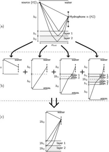
In this case, each reflection on an interface关Fig.6共a兲兴 is identified by the receiver array as an image source which can be described in an equivalent system: the structure 共water + sediment layers兲 above this interface and its symmetric structure 关Fig.6共b兲兴. So, each image is represented in a dif-ferent equivalent system but, for any given system, the places of the components共water and layer and their symmet-ric structure兲 have no consequences on the angle of arrival or on the total travel time. It is then possible to merge all the equivalent systems in a single one which contains all the FIG. 4. Left: experiment area of the Scarab experiment. Right: sound speed
profile obtained from inversion for site 2共Ref.3兲.
FIG. 5. Temporal signal recorded at the 8thhydrophone of the array.
FIG. 6. Modeling of the seafloor with image sources:共a兲 original configu-ration,共b兲 each reflection on an interface is replaced by its image source, 共c兲 the final equivalent system.
image sources关Fig.6共c兲兴. In this system, all the thicknesses are doubled and the images are located on the interfaces and at a zero horizontal offset relative to the source.
B. Backpropagation of signals
The geoacoustic inversion by the image source method requires a very accurate localization. To solve this problem, the recorded signals are backpropagated numerically in the water without the sediment structure. This can be done in this case because the time t0 of the emission of the wavelet by the source is known and because the time resolution of signal is good enough to separate each reflection共Figs.3and 5兲.
The imaging with backpropagation of signals is very close to the time reversal in a homogeneous media16–19 but signals reflected by the seabed will not focus only on the real source after backpropagation like in the physical time reversal.20 They will also focus on all image sources corre-sponding to the reflections on geological interfaces because the sediment structure is suppressed. This phenomenon has already been shown during a time reversal experiment21but here, it is used to characterize the seafloor. Source and im-ages are coherent because they emit the same signal 共with different amplitudes兲 at time t0.
For a monopole emitting a short pulse f共t兲 at r0s in a homogeneous and isotropic medium, the received signal at hydrophone n at rnr is sn共t兲 = f共t兲 ⴱ g共r0 s ,rn r,t兲 + n共t兲, 共3兲
whereⴱ is the convolution product, g共r0s, rn
r, t兲 the temporal
domain Green’s function, and n共t兲 an additive supposed
spatially white noise.
If M + 1 monopole sources 共the real one+M images兲 emit the same wavelet at the same time with a different am-plitude factor m, the received signal becomes
sn共t兲 =
兺
m=0 M mf共t兲 ⴱ g共rm s ,rn r,t兲 + n共t兲, 共4兲or in the frequency domain Sn共兲 =
兺
m=0 M mF共兲 ⫻ G共rm s ,rn r ,兲 +n共兲, 共5兲 with G共rm s , rn r,兲 and F共兲 the Fourier transforms of g共r0s, rn
r, t兲 and f共t兲.
To backpropagate signals at a search point r, the spectrum Sn共兲 is multiplied by the inverse Green
function in an homogeneous medium共with sound speed c0兲 G0−1共r,rn r ,兲=兩r−rn r兩⫻e−i共共兩r−rnr兩兲/c0兲 : Sbn共r,兲 =
冋
兺
m=0 M mF共兲 ⫻ G共rm s ,rn r ,兲 +n共兲册
⫻ G0 −1共r,r n r ,兲. 共6兲In order to reduce the influence of all sources and the noise, the backpropagated signals are windowed around t0 with a smooth window w共t兲 that has nearly the same duration than
the emitted wavelet. In the frequency domain, the windowed backpropagated signal is
Swn共r,兲 = Sbn共r,兲 ⴱ FT关w共t兲兴. 共7兲
Then, the average of the N hydrophones of the array is com-puted and the result共homogeneous to a pressure兲 is mapped as follows: IBW共r兲 =
冑
冕
−⬁ +⬁冏
1 N兺
n Swn共r,兲冏
2 d. 共8兲Equivalently,IBW共r兲 can be noted as a sum of the covariance matrix elements: IBW共r兲 =
冑
冕
−⬁ +⬁ 1 N兺
n=1 N兺
q=1 N Swn共r,兲Swqⴱ 共r,兲d, 共9兲where Swnⴱ 共r,兲 is the conjugate of Swn共r,兲.
IBW is very close to the Kirchhoff migration but here,
instead of migrating signals on the reflectors, they are mi-grated to the image source locations.
Even with the window, there is still speckle on IBW.
Indeed, the wavelet emitted by the source m and received by the sensor n draws a circle on the map centered on the sensor with a radius of兩r0s− rn
r兩. The intersection of the circles of the
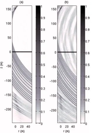
N sensors corresponds to the location of a source. The prob-lem is that it is possible for some isolated circles to be greater than a coherent intersection of circles corresponding to another source with a lower amplitude. This is visible on Figs.7共a兲and7共b兲where the functionalIBW共r兲 is computed respectively for synthetic and real data. For the synthetic data, the map clearly shows the sources but also all the circles drawn by all the individual hydrophones as men-tioned. The same result is observed on SCARAB data 关Fig. 7共b兲兴 where the image obtained with IBW共r兲 shows even
more artifacts. This may have been caused by the presence of another sound-emitting object共maybe a merchant ship兲 near the experiment area. With this map of image sources, it is difficult to locate them accurately.
C. Projection onto the orthogonal subspace and range estimation
The source amplitudes are not required for localization. Consequently the backpropagated and windowed signals can be normalized and projected onto the orthogonal subspace 共I−关Sw共r,兲/储Sw共r,兲储2,N兴关Sw
H共r,兲/储S
w共r,兲储2,N兴兲. Then, source locations correspond to the minima of the function
FOS共r,兲 = IH
冉
I − Sw共r,兲 储Sw共r,兲储2,N Sw H共r,兲 储Sw共r,兲储2,N冊
I 共10兲 or FOS共r,兲 = N −兺
n=1 N兺
q=1 N Swn共r,兲 储Sw共r,兲储2,N ⫻ Swqⴱ 共r,兲 储Sw共r,兲储2,N , 共11兲 where subscript Hdenotes the Hermitian transpose,Sw共r,兲 =
冢
Sw1共r,兲 Sw2共r,兲 ] SwN共r,兲冣
,储·储2,Nis the L2norm of the signal vector, I is identity matrix andI a column vector of ones.
One can note the similarity between Eq. 共10兲 and the MUltiple SIgnal Classification 共MUSIC兲22 algorithm. Here, the vectors of Green’s function are replaced by vectors of ones because vectors of signals Sw are already
backpropa-gated. Thus, Swwith its normalization and windowing can be
interpreted as a user-selected set of eigenvectors of the sig-nals. This is possible here because all reflected pulses in the temporal signal are in the same order for each sensor. The advantage of this method is that there is no limitation of the number of sources detectable in opposition to the MUSIC algorithm in which it is impossible to find more sources than the number of sensors. In the MUSIC algorithm with wide-band sources, the information of the eigenvectors is redun-dant as a function of frequency even if several echoes with different arrival times are visible by eye on the temporal signal 共see Fig. 3兲. The range resolution of FOS is directly
linked to the window size w共t兲. To improve the accuracy of the range resolution, we use the knowledge of the emitted wavelet F共兲 by comparing it with the average of the
back-propagated and windowed signals. This comparison is very close to an arrival time analysis of the emitted pulse. For this operation, the function to minimize is
FAT共r,兲 = min ⫾
冏
Fw共兲 储fw共t兲储⬁,t ⫾ 1 N兺
n Swn共r,兲 储swn共r,t兲储⬁,t冏
2 , 共12兲 with fw共t兲= f共t兲⫻w共t兲, Fw共兲=FT关fw共t兲兴, swn共r,t兲=FT−1关Swn共r,兲兴 and 储·储⬁,t is the infinite norm of the signal
over the time. The minimum is taken between addition and subtraction because the reflection coefficient may be positive or negative. Finally, the image sources are mapped with the function IOSAT共r兲 = 1
冕
−⬁ +⬁ 兩Fw共兲兩2FOS共r,兲 + FAT共r,兲d , 共13兲whereFOS共r,兲 is compensated in frequency with the power
spectrum of the emitted pulse.
The results of the function IOSAT共r兲 关Eq. 共13兲兴 are
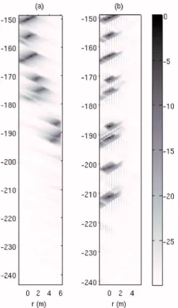
dis-played on Fig.8共a兲for synthetic data and on Fig.8共b兲for the at-sea data.
This new function eliminates all the circles drawn with IBW共r兲 关Eq. 共9兲兴 and the image sources appear very clearly
and with a good resolution both in range and angle. Because of the low frequency regime of the source, it appears from the map obtained with real data that phase shifting from dispersion phenomena is not strong enough to influence FAT共r兲 and reduce the quality of the detected images. On this
SCARAB data result, fewer image sources appear on the FIG. 7. 共Color online兲 Focus on the image sources using IBWfor共a兲 the
synthetic model and 共b兲 the SCARAB data. The source is at 共r=0, z = 150兲 and the solid line at z=0 represents the seafloor. The array is not drawn on the picture and is at r = 200 m.
FIG. 8. 共Color online兲 Focus on the image sources using IOSAT共r兲 共in dB兲
map than expected from the knowledge of the geoacoustic structure of the seafloor共made of 20 layers with a total thick-ness of 150 m兲 because some of the layers are very thin and their corresponding image sources are merged in a single spot. The map obtained with synthetic data shows more than ten image sources, some of them correspond to multiple re-flections between interfaces. On the temporal signal they cor-respond to very low amplitude echoes that could be hidden by a faint noise. Nevertheless, their amplitudes on the map are lower than images corresponding to the first reflections and can be eliminated from the automated detection by ad-justing a threshold. One can note on the maps that the image sources are not aligned on a perfect straight line; this is due to the refraction in the sediment layer共cf. Figure 6兲 that is not yet taken into account in the detection algorithm. IV. SOUND SPEED PROFILE MEASUREMENT
As described in Section III C, image sources are not aligned on the vertical axis because signals are backpropa-gated in water without sediment structure. To find the layer sound speed, image sources must be aligned on the vertical axis of the real source. This vertical axis is the line between the real source and the first image, meaning that finding the real source and the first image makes it possible to calculate the array tilt and correct it.
A. Correction of the array tilt
Because of currents, it is possible for the vertical array to be deformed. If one assumes that the deformation is mainly a tilt, the array makes an angle␣with the vertical. If this angle is not included in the coordinates of the hydro-phones, the line between the real source and the first image forms an angle—␣with the real vertical line. Thus, the new coordinates of the hydrophones rn
r␣
=共rn r␣
, zn
r␣兲 that include
the tilt are rn r␣ = rn r cos␣− zn r sin␣, zn r␣ = rn r sin␣+ zn r cos␣, 共14兲 with −␣= tan−1r0 s − r1s z0s− z1s. 共15兲 共r0 s
, z0s兲 and 共r1s, z1s兲 are respectively the real source and the first image’s coordinates found with the tilted array.
The array tilt is usually an unknown parameter and is easily recovered here with the image source method. After tilt correction, image sources can be aligned on the vertical real source axis to recover the sound speed profile. Note that the vertical axis is not perpendicular to the sea surface but to the seabed.
B. Image source alignment
When IOSAT共r兲 关Eq. 共13兲兴 is computed with correct
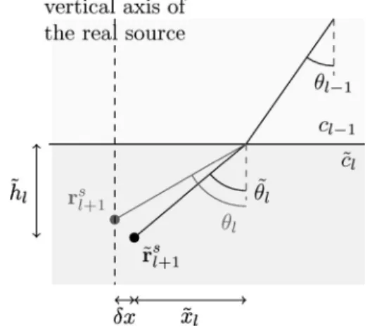
sound speeds from c0to cl−1and a wrong one c˜lin layer l the
共l+1兲th image is located at r =共r˜ l+1 s , z˜l+1s 兲 with r˜ l+1 s ⫽r 0 s 共Fig.
9兲. The ˜ symbol indicates an incorrect value.
The range gap ␦x = r˜l+1s − r0s, the apparent depth h˜l, and
the angle of arrival on the array center0of this image give all the necessary information to find the real sound speed in the layer. The Snell-Descartes law allows one to obtain the arrival angle˜l on the image source:
˜ l= sin−1
冉
c ˜l c0sin0冊
, 共16兲then, the horizontal travel x˜lin the layer is
x
˜l= h˜ltan˜l, 共17兲
and the travel time in the layer tlis
tl= h ˜ l c ˜lcos˜l . 共18兲
Even if˜l, h˜land c˜lare incorrect, tlis the correct travel
time in the layer for that ray because of the backpropagation procedure. The real horizontal travel in the layer that is xl
= x˜l+␦x is also known. With these two quantities and the
Snell-Descartes law, it is now possible to write sin0 c0 = sin˜l c ˜l =sin ˆ l cˆl =共x˜l+␦x兲 tlcˆl 1 cˆl , 共19兲
where the symbol ˆ indicates an estimated value. Thus, the estimated sound speed in the layer l is
cˆl=
冑
共x˜l+␦x兲c0 tlsin0
. 共20兲
The estimation is due to the ray path approximated as com-ing from the array center.
C. Focus in layers
To compute IOSAT共r兲 关Eq.共13兲兴 taking into account the
layer sound speeds c0, . . . , cl−1, cˆl, the inverse Green’s
func-tion that takes into account the refracfunc-tion in layers is ap-proximated by
FIG. 9. Image sources gap to the vertical of the real source.
G−1共rn r ,r,兲 = Dtot共rn r,r兲 ⫻ e−i⌬t共r n r,r兲 , 共21兲 where Dtot共rn
r, r兲 is the path length between r n r
and r共Fig.10兲 and⌬t共rn
r, r兲 is the travel time. The expressions of D tot and ⌬t are6 Dtot=
兺
p=0 l hp cosp =兺
p=0 l hp冑
1 −冉
cp c0 sin0冊
2, 共22兲 ⌬t =兺
p=0 l hp cpcosp =兺
p=0 l hp cp⫻冑
1 −冉
cp c0 sin0冊
2, 共23兲where hpandp are respectively the thickness and the
inci-dence angle of the layer p共Fig.10兲. To find these values, the initial incidence angle 0 must be known. The horizontal distance covered by a ray between two different horizontal planes is6 x共0兲 =
兺
p=0 l hptanp=兺
p=0 l hp cp c0 sin0冑
1 −冉
cp c0 sin0冊
2, 共24兲and the horizontal travel between rn r =共rn r, z兲 and r=共r,z兲 is xtot=兩rn r− r兩. Then, 0 is found by solving x共0兲 − xtot= 0. 共25兲
Then the inverse Green’s function关Eq. 共21兲兴 is used for the backpropagation of signals in Eq.共6兲.
D. Algorithm
Once the tilt is corrected and the first image is found with IOSAT共r兲, the first layer sound speed c˜
1 is initialized
with that of water. When the second image is located, cˆ1is calculated andIOSAT共r兲 restarts the search of the second im-age with this new sound speed of the first layer. Then, if␦x of the second image is still different from zero, cˆ1 becomes c
˜1 and a new estimate cˆ1is calculated. This process is done until␦x = 0. Then cˆ1becomes c1 and c˜2is initialized with c1 and the operation is repeated for each layer.
E. Results
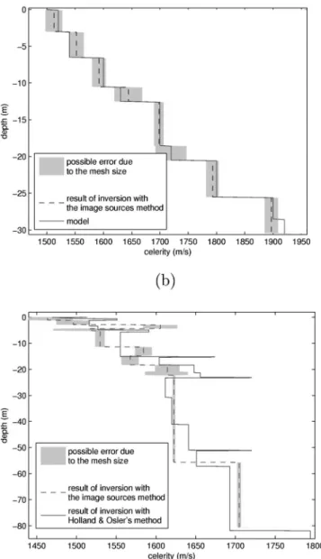
In order to recover the sound speed profile, image sources have to be precisely located. This is done using a dense spatial mesh. Here the density of the mesh is one node each 10 cm 共a tenth of the wavelength at the central fre-quency兲 on the ray coming from the array center and these ray paths cross the vertical source axis every 10 cm. Then the alignment of images 共Fig. 11兲 allows one to recover the sound speed profile. It is correctly recovered for the synthetic data where only the 9thinterface is not found because of its low impedance contrast关Fig.12共a兲兴.
Ground truth from SCARAB experiment3 has been ob-tained for the 6 first meters which is not enough to compare with the sound speed profile obtained with the image source method. So the result is compared with that of Holland and Osler. They obtained 20 layers共labeled with numbers from 1 to 20 in TableII兲 while the image source method obtains 11 layers共labeled with letters from a to k in TableII兲. The first meters of seafloor are complex 共layers 1 to 5兲 with the no-table presence of a thin surficial layer with a sound-speed gradient starting with a sound speed lower than water. In these first meters, the image source method gives 4 layers共a FIG. 10. Refraction of ray in layered media.
FIG. 11.共Color online兲 Image sources before 共a兲 and after 共b兲 alignment for the synthetic data.
to d兲 which depths match correctly with layers 2 to 5. How-ever, the inverted speed profile is different from that of Hol-land and Osler. One can note that the two first layers共a and b兲 are found with a low sound speed which may corresponds to the surficial layer. Two layers共e and f兲 found by the image source method correspond to a single one共layer 6兲. Layers 7, 11, and 15 are not found probably because of their thinnesses 共20 cm兲. Layers 8 to 10 are correctly enough found by image source method共layers g to i兲, the thickness differences being lower than 60 cm and the sound-speed differences being lower than 42 m/s−1. Layers 12 to 16 are merged in a single layer j. The obtained sound speed for layer j corresponds within an uncertainty of 10 m/s−1to the mean sound speed of layers 12 to 16. The fusion of these layers is probably due to a low impedance contrast between successive layers which leads to a too low reflection coefficient to produce a detect-able image source. The agreement between layer 17 and layer k is good for both the thickness and the sound speed.
The deepest layers 18, 19, and 20 are not found with the image source method. Despite these differences, the overall shapes of the sound speed profiles match correctly enough 关Fig. 12共b兲兴 and the profile given by the image source method is obtained without any a priori information about the number of layers, their thicknesses or their sound speed. The sources of error in sound speed values are not stud-ied here but on Fig. 12, the gray zones represent the maxi-mum error for sound speeds when they are computed assum-ing that the maximum in amplitude of a detected image could be badly located and should be on a neighboring node. One can see that when layers are thin, errors are likely be-cause of the mesh size. Among other sources of error, the successive determination of sound speeds in layers involves that a computed sound speed must compensate errors done with previous ones. Also, we suppose that the small size of the Fresnel zones 共⬇70 m兲 in the image source method makes the technique sensitive to the slopes共or low frequency roughness兲 of interfaces. The sensitivity to these parameters is the object of future work.
V. CONCLUSION
The initial results obtained on synthetic and real data with only one transmission between the source and the ver-tical array are promising. The different reflections on the interfaces are well modeled by image sources and the array process is able to locate them accurately enough to obtain the sound speed profile. The comparison of the real data result with another method shows significant differences but the global shapes of the sound speed profiles match correctly FIG. 12. Sound speed profiles found with the synthetic data共a兲 and with the
real data共b兲 共see Ref.3for details兲.
TABLE II. Comparison of results with measured data between Holland’s and image source method.
Holland and Osler’s method Image source method
Layer Thickness 共m兲 Depth 共m兲 Sound speed 共m/s兲 Layer Thickness 共m兲 Depth 共m兲 Sound speed 共m/s兲 1 0.5 0.5 1470–1502 2 0.6 1.1 1551 a 1.1 1.1 1464 3 2.2 3.3 1516 b 1.7 2.8 1496 4 1.5 4.8 1527 c 1.5 4.3 1606 5 0.8 5.6 1591 d 0.8 5.1 1516 e 6.2 11.3 1530 6 9.5 15.1 1555 f 3.5 14.7 1584 7 0.2 15.3 1674 8 3 18.3 1604 g 3.6 18.3 1568 9 3 21.3 1648 h 2.5 20.8 1615 10 1.7 23 1656 i 1.5 22.2 1614 11 0.2 23.2 1720 12 7.5 30.7 1612 13 10.4 41.1 1620 14 9.9 51 1641 15 0.2 51.2 1720 16 6 57.2 1651 j 33.3 55.6 1622 17 24.7 81.9 1693 k 25 80.6 1705 18 68 149.9 1794 19 0.2 150.1 1900 20 ¯ ¯ 1820
enough. The main difference with existing methods is that the process presented here is not based on comparison with a model. It is a data-driven approach which consequently has a low computational cost and is very fast. It could therefore be used as a first step in a more accurate inversion procedure, or to evaluate the geologic structure and the sound speed profile of large areas with the use of a towed horizontal array. The object of future work is to find other parameters like density and low frequency roughness共or local slopes of interfaces兲. ACKNOWLEDGMENTS
The authors wish to gratefully acknowledge Charles W. Holland for providing the data and for helpful discussion and remarks on the manuscript. They also thank the North Atlan-tic Treaty Organization Underwater Research Center under whose auspices the data were collected. This work is par-tially funded by the GIS-Europole Mer research consortium.
1A. Baggeroer, W. Kuperman, and P. Mikhalevsky, “An overview of
matched field methods in ocean acoustics,” IEEE J. Ocean. Eng. 18, 401– 424共1993兲.
2D. Jackson and M. Richardson, High-Frequency Seafloor Acoustics
共Springer, New York, 2007兲, pp. 321–330.
3C. Holland and J. Osler, “High resolution geoacoustic inversion in shallow
water: A joint time and frequency domain technique,” J. Acoust. Soc. Am.
107, 1263–1279共2000兲.
4L. Guillon and C. Holland, “Cohérence des signaux réfléchis par le sol
marin: Modèle numérique et données expérimentales共Coherence of sig-nals reflected by the seafloor: Numerical modeling vs experimental data兲,” Trait. Signal 25, 131–138共2008兲.
5J. Claerbout and S. Doherty, “Downward continuation of
moveout-corrected seismograms,” Geophysics 37, 741–768共1972兲.
6L. Brekhovskikh and Y. Lysanov, Fundamentals of Ocean Acoustics
共Springer-Verlag, Berlin, 1991兲, pp. 74–81.
7L. Brekhovskikh and O. Godin, Acoustics of Layered Media. II: Point
Sources and Bounded Beams共Springer-Verlag, Berlin, 1999兲, pp. 1–15.
8P. Cervanka and P. Challande, “A new efficient algorithm to compute the
exact reflection and transmission factors for plane waves in layered ab-sorbing media共liquids and solids兲,” J. Acoust. Soc. Am. 89, 1579–1589 共1991兲.
9J. Allen and D. Berkley, “Image method for efficiently simulating small
room acoustics,” J. Acoust. Soc. Am. 65, 943–950共1979兲.
10J. Fawcett, “Complex-image approximations to the half-space
acousto-elastic Green’s function,” J. Acoust. Soc. Am. 108, 2791–2795共2000兲.
11J. Fawcett, “A method of images for a penetrable acoustic waveguide,” J.
Acoust. Soc. Am. 113, 194–204共2003兲.
12X. Xu and Y. Huang, “An efficient analysis of vertical dipole antennas
above a lossy half-space,” Electromagn. Waves 74, 353–377共2007兲.
13N. Chapman, J. Desert, A. Agarwal, Y. Stephan, and X. Demoulin,
“Esti-mation of seabed models by inversion of broadband acoustic data,” Acta. Acust. Acust. 88, 756–759共2002兲.
14C. Park, W. Seong, P. Gerstoft, and M. Siderius, “Time-domain
geoacous-tic inversion of high-frequency chirp signal from a simple towed system,” IEEE J. Ocean. Eng. 28, 468–478共2003兲.
15P. Pignot and N. Chapman, “Tomographic inversion of geoacoustic
prop-erties in a range-dependent shallow-water environment,” J. Acoust. Soc. Am. 110, 1338–1348共2001兲.
16P. Roux and W. Kuperman, “Time reversal of ocean noise,” J. Acoust. Soc.
Am. 117, 131–136共2005兲.
17L. Borcea, G. Papanicolaou, C. Tsogka, and J. Berryman, “Imaging and
time reversal in random media,” Inverse Probl. 18, 1247–1279共2002兲.
18L. Borcea, G. Papanicolaou, and C. Tsogka, “Optimal illumination and
wave form design for imaging in random media,” J. Acoust. Soc. Am. 122, 3507–3518共2007兲.
19J. Berryman, L. Borcea, G. Papanicolaou, and C. Tsogka, “Statistically
stable ultrasonic imaging in random media,” J. Acoust. Soc. Am. 112, 1509–1522共2002兲.
20M. Fink, “Time reversal mirrors,” J. Phys. D: Appl. Phys. 26, 1333–1350
共1993兲.
21C. Prada, J. de Rosny, D. Clorennec, J. Minonzio, A. Aubry, M. Fink, L.
Berniere, P. Billand, S. Hibral, and T. Folegot, “Experimental detection and focusing in shallow water by decomposition of the time reversal op-erator,” J. Acoust. Soc. Am. 122, 761–768共2007兲.
22R. Schmidt, “A signal subspace approach to multiple emitter and signal
parameter estimation,” Ph.D. thesis, Stanford University, Stanford, CA 共1981兲.