A surrogate model based on Non-Uniform Rational B-Splines hypersurfaces

(1)

Science Arts & Métiers (SAM)

is an open access repository that collects the work of Arts et Métiers Institute of

Technology researchers and makes it freely available over the web where possible.

This is an author-deposited version published in: https://sam.ensam.eu Handle ID: .http://hdl.handle.net/10985/17332

To cite this version :

Yohann AUDOUX, Marco MONTEMURRO, Jérôme PAILHES - A surrogate model based on Non-Uniform Rational B-Splines hypersurfaces - Procedia CIRP - Vol. 70, p.463-468 - 2018

Any correspondence concerning this service should be sent to the repository Administrator : archiveouverte@ensam.eu

(2)

ScienceDirect

Available online at www.sciencedirect.com Available online at www.sciencedirect.com

ScienceDirect

Procedia CIRP 00 (2017) 000–000

www.elsevier.com/locate/procedia

Peer-review under responsibility of the scientific committee of the 28th CIRP Design Conference 2018.

28th CIRP Design Conference, May 2018, Nantes, France

A new methodology to analyze the functional and physical architecture of

existing products for an assembly oriented product family identification

Paul Stief *, Jean-Yves Dantan, Alain Etienne, Ali Siadat

École Nationale Supérieure d’Arts et Métiers, Arts et Métiers ParisTech, LCFC EA 4495, 4 Rue Augustin Fresnel, Metz 57078, France

* Corresponding author. Tel.: +33 3 87 37 54 30; E-mail address: paul.stief@ensam.eu

Abstract

In today’s business environment, the trend towards more product variety and customization is unbroken. Due to this development, the need of agile and reconfigurable production systems emerged to cope with various products and product families. To design and optimize production systems as well as to choose the optimal product matches, product analysis methods are needed. Indeed, most of the known methods aim to analyze a product or one product family on the physical level. Different product families, however, may differ largely in terms of the number and nature of components. This fact impedes an efficient comparison and choice of appropriate product family combinations for the production system. A new methodology is proposed to analyze existing products in view of their functional and physical architecture. The aim is to cluster these products in new assembly oriented product families for the optimization of existing assembly lines and the creation of future reconfigurable assembly systems. Based on Datum Flow Chain, the physical structure of the products is analyzed. Functional subassemblies are identified, and a functional analysis is performed. Moreover, a hybrid functional and physical architecture graph (HyFPAG) is the output which depicts the similarity between product families by providing design support to both, production system planners and product designers. An illustrative example of a nail-clipper is used to explain the proposed methodology. An industrial case study on two product families of steering columns of thyssenkrupp Presta France is then carried out to give a first industrial evaluation of the proposed approach.

Keywords: Assembly; Design method; Family identification

1. Introduction

Due to the fast development in the domain of communication and an ongoing trend of digitization and digitalization, manufacturing enterprises are facing important challenges in today’s market environments: a continuing tendency towards reduction of product development times and shortened product lifecycles. In addition, there is an increasing demand of customization, being at the same time in a global competition with competitors all over the world. This trend, which is inducing the development from macro to micro markets, results in diminished lot sizes due to augmenting product varieties (high-volume to low-volume production) [1]. To cope with this augmenting variety as well as to be able to identify possible optimization potentials in the existing production system, it is important to have a precise knowledge

of the product range and characteristics manufactured and/or assembled in this system. In this context, the main challenge in modelling and analysis is now not only to cope with single products, a limited product range or existing product families, but also to be able to analyze and to compare products to define new product families. It can be observed that classical existing product families are regrouped in function of clients or features. However, assembly oriented product families are hardly to find.

On the product family level, products differ mainly in two main characteristics: (i) the number of components and (ii) the type of components (e.g. mechanical, electrical, electronical).

Classical methodologies considering mainly single products or solitary, already existing product families analyze the product structure on a physical level (components level) which causes difficulties regarding an efficient definition and comparison of different product families. Addressing this

Procedia CIRP 70 (2018) 463–468

Peer-review under responsibility of the scientific committee of the 28th CIRP Design Conference 2018. 10.1016/j.procir.2018.03.234

ScienceDirect

Procedia CIRP 00 (2017) 000–000 www.elsevier.com/locate/procedia

28th CIRP Design Conference, May 2018, Nantes, France

A surrogate model based on Non-Uniform Rational B-Splines

hypersurfaces

Y. Audoux

a

_{, M. Montemurro}

a,

_{*, J. Pailhes}

a

a_{Arts et Métiers ParisTech, I2M, CNRS UMR 5295,Esplanade des Arts et Métiers, F-33400 Talence, France}

* Corresponding author. Tel.: +33-556-845-333. E-mail address: marco.montemurro@ensam.eu

Abstract

This study aims at providing an original metamodeling technique based on the Non-Uniform Rational B-Splines (NURBS) formalism. The proposed approach is able to fit general non-convex sets of target points (TPs) by extending the NURBS formalism to the N-dimensional (N-D) case, getting in this way a general NURBS hypersurface. The shape of such a hypersurface is tuned by several parameters: the number of control points (CPs), their coordinates and related weights, the degrees of the blending functions and the knot-vector components defined along each direction. The goal of the proposed strategy is to find the best NURBS hypersurface approximating a given set of TPs. To this purpose the problem is formulated as an unconstrained least-square distance problem wherein the optimisation variables are all the parameters tuning the shape of the NURBS hypersurface. Nevertheless, when the number of CPs and the degrees of the basis functions are included among the design variables the resulting problem is defined over a space having a variable dimension. To deal with this aspect, a special genetic algorithm, able to solve problems characterised by a variable number of design variables, is considered to determine automatically (i.e. without the user’s intervention) the optimum value of both the design space size (related to the integer variables of the NURBS hypersurface) and the NURBS hypersurface continuous parameters. The effectiveness of the proposed approach is proven by means of a meaningful benchmark.

Keywords: Optimization ; Genetic Algorithme ; NURBS ;

1. Introduction

Computers increasing performances are widely utilized to improve simulation complexity over computation time. However, some applications need quasi-real-time models especially for design/optimisation purposes. Metamodeling techniques can minimise the computational effort to realize complex multi-field and/or multi-scale simulations which must be integrated within an optimisation process. Currently, Artificial Neural Networks (ANN) [1,2], Proper Generalized Decomposition (PGD) [3], Fuzzy Logic (FL) [4] and Radial Basis Functions (RBFs) [5] are the most common methods available in literature for realising surrogate models. Of course, each technique is characterised by both advantages and shortcomings. For example, ANN are not suitable for multiple outputs request [2] (when considering multiple responses ANN

accuracy often decreases), while PGD provides less accurate results for nonlinear problems [3]. As a general remark, setting the parameters number for classical metamodeling techniques could be a quite difficult task which often needs a trial-and-error approach. For instance, improving arbitrarily the number of layers and/or neurons for ANN or improving the modes number for PGD can lead to overfitting and to a subsequent increase of the overall complexity for the problem at hand. In any case, all these methods need a great amount of available data, thus implying extensive experimental and/or numerical campaigns.

The surrogate model proposed in this study relies on the utilisation of N-dimension (N-D) Non-Uniform Rational Basis Spline (NURBS) hypersurfaces to fit a given set of data points, also called target points (TPs) and aims at overcoming the previous limitations by automatically determining the optimum

Available online at www.sciencedirect.com

ScienceDirect

Procedia CIRP 00 (2017) 000–000 www.elsevier.com/locate/procedia

28th CIRP Design Conference, May 2018, Nantes, France

A surrogate model based on Non-Uniform Rational B-Splines

hypersurfaces

Y. Audoux

a

_{, M. Montemurro}

a,

_{*, J. Pailhes}

a

a_{Arts et Métiers ParisTech, I2M, CNRS UMR 5295,Esplanade des Arts et Métiers, F-33400 Talence, France}

* Corresponding author. Tel.: +33-556-845-333. E-mail address: marco.montemurro@ensam.eu

Abstract

This study aims at providing an original metamodeling technique based on the Non-Uniform Rational B-Splines (NURBS) formalism. The proposed approach is able to fit general non-convex sets of target points (TPs) by extending the NURBS formalism to the N-dimensional (N-D) case, getting in this way a general NURBS hypersurface. The shape of such a hypersurface is tuned by several parameters: the number of control points (CPs), their coordinates and related weights, the degrees of the blending functions and the knot-vector components defined along each direction. The goal of the proposed strategy is to find the best NURBS hypersurface approximating a given set of TPs. To this purpose the problem is formulated as an unconstrained least-square distance problem wherein the optimisation variables are all the parameters tuning the shape of the NURBS hypersurface. Nevertheless, when the number of CPs and the degrees of the basis functions are included among the design variables the resulting problem is defined over a space having a variable dimension. To deal with this aspect, a special genetic algorithm, able to solve problems characterised by a variable number of design variables, is considered to determine automatically (i.e. without the user’s intervention) the optimum value of both the design space size (related to the integer variables of the NURBS hypersurface) and the NURBS hypersurface continuous parameters. The effectiveness of the proposed approach is proven by means of a meaningful benchmark.

Keywords: Optimization ; Genetic Algorithme ; NURBS ;

1. Introduction

Computers increasing performances are widely utilized to improve simulation complexity over computation time. However, some applications need quasi-real-time models especially for design/optimisation purposes. Metamodeling techniques can minimise the computational effort to realize complex multi-field and/or multi-scale simulations which must be integrated within an optimisation process. Currently, Artificial Neural Networks (ANN) [1,2], Proper Generalized Decomposition (PGD) [3], Fuzzy Logic (FL) [4] and Radial Basis Functions (RBFs) [5] are the most common methods available in literature for realising surrogate models. Of course, each technique is characterised by both advantages and shortcomings. For example, ANN are not suitable for multiple outputs request [2] (when considering multiple responses ANN

accuracy often decreases), while PGD provides less accurate results for nonlinear problems [3]. As a general remark, setting the parameters number for classical metamodeling techniques could be a quite difficult task which often needs a trial-and-error approach. For instance, improving arbitrarily the number of layers and/or neurons for ANN or improving the modes number for PGD can lead to overfitting and to a subsequent increase of the overall complexity for the problem at hand. In any case, all these methods need a great amount of available data, thus implying extensive experimental and/or numerical campaigns.

The surrogate model proposed in this study relies on the utilisation of N-dimension (N-D) Non-Uniform Rational Basis Spline (NURBS) hypersurfaces to fit a given set of data points, also called target points (TPs) and aims at overcoming the previous limitations by automatically determining the optimum

(3)

464 Y. Audoux et al. / Procedia CIRP 70 (2018) 463–468

2 Author name / Procedia CIRP 00 (2018) 000–000

number of the NURBS hypersurface parameters without requiring a trial-and-error approach.

Up to now, only few research works focus on the formulation/implementation of surrogate models based on the NURBS formalism [6–8]. NURBS curves and surfaces are standard geometrical entities widely used in Computer Aided Design (CAD) software. NURBS hypersurfaces represent a generalisation of these entities. A NURBS hypersurface is defined through the number of dimensions (related to the size of the problem at hand), the degree of blending-functions along each dimension, the overall number of control points (CPs), the coordinates of each CPs and the related weights, the knot vector components along each dimension. The large number of parameters tuning the shape of a NURBS hypersurface renders it a very versatile tool for many mathematical and engineering applications, not only for formulating surrogate models [9–12]. However, the significant amount of parameters defining the NURBS hypersurface also constitutes the main drawback: it is very hard to properly tune all these parameters without making some simplifying assumptions or preliminary choices as done in[6,7].

In [8] a NURBS-based surrogate model for inverse characterization of composite materials is presented. In this background Turner and Crawford [6] developed an iterative procedure for determining a suitable number of CPs for the NURBS hypersurface. The technique proposed by Turner and Crawford is based upon an empirical rule which computes the position of new control points on the basis of the cost function of the problem at hand (typically the maximum error of approximation). Nevertheless, their approach is characterised by some restrictions:

 the empirical rule for updating the number of CPs as well as their coordinates is strongly problem-dependent;  the degrees of blending functions were set a priori;  the knot vectors components were uniformly distributed

or calculated by means of simple empirical rules.

To overcome the previous restrictions, in this work, an innovative surrogate model based on N-D NURBS hypersurfaces is proposed. The problem of approximating a given set of TPs is formulated as an unconventional Unconstrained Non-Linear Programming Problem (UNLPP) defined over a space of variable dimension. Furthermore, this UNLPP is formulated without considering simplifying hypotheses, thus by considering as design variables all the parameters tuning the NURBS hypersurface shape (both

integer and continuous parameters).

Of course, when dealing with an optimisation problem defined over a domain having a variable dimension, a particular care must be put in the choice of a proper numerical tool to perform the solution search. To this purpose in this study a special genetic algorithm (GA) [11,13] able to deal with problems characterised by a “variable number of design variables” is utilised as optimisation tool.

The effectiveness of the proposed approach will be proven through a meaningful benchmark.

2. A NURBS-based surrogate model

2.1. Classic NURBS surfaces theoretical framework

Non-Uniform Rational B-Splines curves and surfaces are explicit parametric geometric entities mostly used in CAD software. According to the notation introduced in [14] the Cartesian coordinates of a generic point of a NURBS surface can be written as:

𝑺𝑺(𝑢𝑢, 𝑣𝑣) = ∑𝑛𝑛𝑢𝑢𝑖𝑖=0∑𝑛𝑛𝑣𝑣𝑗𝑗=0𝑁𝑁𝑖𝑖,𝑝𝑝(𝑢𝑢)𝑁𝑁𝑗𝑗,𝑞𝑞(𝑣𝑣)𝜔𝜔𝑖𝑖,𝑗𝑗𝑷𝑷𝑖𝑖,𝑗𝑗

∑𝑛𝑛𝑢𝑢_𝑖𝑖=0∑𝑛𝑛𝑣𝑣_𝑗𝑗=0𝑁𝑁𝑖𝑖,𝑝𝑝(𝑢𝑢)𝑁𝑁𝑗𝑗,𝑞𝑞(𝑣𝑣)𝜔𝜔𝑖𝑖,𝑗𝑗 , (1)

where

u

, 

v

 

0 ,

1

are the dimensionless parameters of the surface,

S





3 is the vector collecting the coordinates of the generic point belonging to the surface, whilst

P

_i,_jis the array of the CPs coordinates, i.e. one array of size



nu1  nv1 is required for each coordinate.



n

_u



1 

and



n

_v



1 

are the number of CPs along

u

and

v

directions, respectively.

 1  1 ,   





nu nv j i



is the array of weights related to each CP.

N

_i_,_p

(

u

)

and

N

_j_,_q

(

v

)

are the p-th and q-th -degree B-spline blending functions, which are recursively defined. For example, the expression of

N

i,p

(

u

)

is written as:

. ,..., 1 , ,..., 0 ), ( ) ( ) ( , otherwise 0 , if 1 ) ( 1 ,1 1 1 1 1 , , 1 0 , p n i u N U UU u u N U Uu U u N U u U u N u i i i i i i i i i i i i                                (2)

Similar expressions apply for

N

i,q

(

v

)

. In Eq. (2)

U

i is the

i-th component of i-the non-periodic non-uniform knot vector along u direction. Of course, a knot vector is required also in v-direction in order to define the associated blending functions. The generic expression for both knot vectors is:

𝐔𝐔 = {0, … ,0⏟ 𝑝𝑝+1 , 𝑈𝑈𝑝𝑝+1, … , 𝑈𝑈𝑚𝑚𝑢𝑢−𝑝𝑝−1, 1, … ,1⏟ 𝑝𝑝+1 } , 𝐕𝐕 = {0, … ,0⏟ 𝑞𝑞+1 , 𝑈𝑈𝑞𝑞+1, … , 𝑈𝑈𝑚𝑚𝑣𝑣−𝑞𝑞−1, 1, … ,1⏟ 𝑞𝑞+1 } . (3)

The size of knot vectors U and V are



m

_u



1 

and



m

_v



1 

, respectively. Their size strictly depends upon the number of CPs as well as on the degrees of blending functions along each direction, namely

.

1 ,

1 









q

n

m

p

n

m

v v u u (4) Each knot vector is a non-decreasing sequence of real numbers that can be interpreted as a discrete collection of values of the dimensionless parameter of the surface. All the components of knot vectors can have a multiplicity µ. If a knot has a

Author name / Procedia CIRP 00 (2018) 000–000 3

multiplicity µ along u-direction then the basis function

)

(

,

u

N

ip is p-µ times continuously differentiable (at the knot).

The same considerations can be repeated for

N

i,q

(

v

)

if a

component of V has multiplicity µ. Therefore, for a fixed degree along a given direction, increasing the knot multiplicity decreases the continuity of the surface at that knot. This means that the value of the knot vectors components strongly affects the local shape of a NURBS surface. For a deeper insight in the matter, the reader is addressed to [14].

2.2. The case of NURBS hypersurfaces

Let N be the dimension of the problem and M that of the hypersurface. Let

S

:



N





M be the parametric vector equation of the hypersurface. Analogously to the 2D case, the explicit parametric expression of the k-th coordinate of the NURBS hypersurface writes:

M u N u N P u N u N u u S N N N N N N N N N N N i i n i n i i p i p N k i i i i n i n i i p i p N N k _,_k ₁_,..., ) ( )... ( ... ) ( )... ( ... ) ,..., ( ,..., 0 0 , 1 , ) ( ,..., ,..., 0 0 , 1 , 1 ) ( 1 1 1 1 1 1 1 1 1 1 1  

 

      (5)

In Eq. (5),

u

₁

,...,

u

_N

,



 

0 ,

1

are the dimensionless parameters of the hypersurface, while

S

 k is the k-th coordinate of the generic point belonging to the hypersurface.

   1 ... 1 ,..., 1 1    



 N N n n k i i

P is the generic component of the array collecting the k-th coordinate for each CP.



n

_i



1 

is the number of CPs along the i-th dimension, while













N i

n

i

n

1

CP

1

is the overall number of CPs which form the so-called hyper-net. _,...,  1 1 ... 1

1    





N N n n i i



is the

generic component of the array of weights related to each CP. The expression of the generic

p

_i-th degree blending function along dimension i can be stated as:

𝑁𝑁𝑗𝑗,0(𝑢𝑢𝑖𝑖) = {1 if 𝑈𝑈𝑗𝑗 (𝑖𝑖)_{≤ 𝑢𝑢} 𝑖𝑖≤ 𝑈𝑈𝑗𝑗+1(𝑖𝑖) 0 otherwise , 𝑁𝑁𝑗𝑗,𝜏𝜏(𝑢𝑢𝑖𝑖) = 𝑢𝑢𝑖𝑖−𝑈𝑈𝑗𝑗(𝑖𝑖) 𝑈𝑈_{𝑗𝑗+𝜏𝜏}(𝑖𝑖)−𝑈𝑈_𝑗𝑗(𝑖𝑖)𝑁𝑁𝑗𝑗,𝜏𝜏−1(𝑢𝑢𝑖𝑖) + 𝑈𝑈_{𝑗𝑗+𝜏𝜏+1}(𝑖𝑖) −𝑢𝑢𝑖𝑖 𝑈𝑈_{𝑗𝑗+𝜏𝜏+1}(𝑖𝑖) −𝑈𝑈_𝑗𝑗+1(𝑖𝑖) 𝑁𝑁𝑗𝑗+1,𝜏𝜏−1(𝑢𝑢𝑖𝑖), (6) 𝑖𝑖 = 1, … , 𝑁𝑁, 𝑗𝑗 = 0, … , 𝑛𝑛𝑖𝑖, 𝜏𝜏 = 1, … , 𝑝𝑝.

Of course, blending functions are defined by considering knot vectors component along each dimension. The expression of the generic knot vector along dimension i is

𝐔𝐔(𝑖𝑖)_{= {0, … ,0}_⏟ 𝑝𝑝𝑖𝑖+1

, 𝑈𝑈_𝑝𝑝(𝑖𝑖)_𝑖𝑖₊₁, … , 𝑈𝑈_𝑚𝑚(𝑖𝑖)_𝑖𝑖_−𝑝𝑝_𝑖𝑖₋₁, 1, … ,1⏟ 𝑝𝑝𝑖𝑖+1

}, (7) where the size of the knot vector is given by

. 1 i , 1 ,...,N p n mi i i  (8)

3. Optimization problem formulation

3.1. Problem description

The problem under consideration here focuses on the approximation of the temperature field of a thin plate of size

1 .

0 

x

L

m and

L

_y



0 .

1

m along x and y axes, respectively. The thickness of the plate is 𝑡𝑡. A constant flux 𝛷𝛷0= 100 W/m² is applied at x = 0 and x = Lx while the rest of the plate is under

convection flux with coefficient

h

and infinite temperature

15 ,

298 



T

K. A pictorial representation is given in Fig. 1. As stated above, the proposed NURBS-based surrogate model aims at approximating the temperature field of the plate for different combinations of variables 𝑡𝑡 and

h

which can be seen as design parameters for the problem at hand. Therefore, the temperature field needs to be determined for each value of the previous parameters, namely:

𝑇𝑇 = 𝑓𝑓(𝑥𝑥, 𝑦𝑦, 𝑡𝑡, ℎ) (9) The goal is thus to determine a suitable NURBS hypersurface fitting (with a certain level of accuracy) a set of given TPs. These TPs must be calculated for different values of 𝑡𝑡 and

h

in each point of the plate. For the considered example the overall dimensions of the NURBS hypersurface are N=4 and M=1, i.e., the NURBS hypersurface reduces to a scalar function depending on four independent parameters as stated in Eq. (9).

The TPs coordinate (i.e. the temperature) can be collected into a N-D array:

𝑄𝑄𝑖𝑖1,𝑖𝑖2,𝑖𝑖3,𝑖𝑖4 = 𝑇𝑇(𝑥𝑥𝑖𝑖1, 𝑦𝑦𝑖𝑖2, 𝑡𝑡𝑖𝑖3, ℎ𝑖𝑖4), ∀𝑖𝑖𝑗𝑗∈ [0 ; 𝑟𝑟𝑗𝑗] (10)

rj+1 being the number of TPs along dimension j. The set of

TPs is composed of an overall number nQ of points given by:

.)

1 (

1 TP









N j j

r

n

(11)

Fig. 1. Geometry and boundary conditions for the plate.

The set of TPs (i.e. the temperature field in each point of the plate for different combinations of 𝑡𝑡 and

h

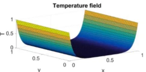
) has been obtained by means of a finite element (FE) analysis. The FE model has been coded into ANSYS environment and it is composed of 101x101 Shell131 elements with a single DOF per node. Fig. 2 illustrates the trend of the temperature field (dimensionless) over the plate for a given pair of thickness and convection coefficient values.

(4)

number of the NURBS hypersurface parameters without requiring a trial-and-error approach.

Up to now, only few research works focus on the formulation/implementation of surrogate models based on the NURBS formalism [6–8]. NURBS curves and surfaces are standard geometrical entities widely used in Computer Aided Design (CAD) software. NURBS hypersurfaces represent a generalisation of these entities. A NURBS hypersurface is defined through the number of dimensions (related to the size of the problem at hand), the degree of blending-functions along each dimension, the overall number of control points (CPs), the coordinates of each CPs and the related weights, the knot vector components along each dimension. The large number of parameters tuning the shape of a NURBS hypersurface renders it a very versatile tool for many mathematical and engineering applications, not only for formulating surrogate models [9–12]. However, the significant amount of parameters defining the NURBS hypersurface also constitutes the main drawback: it is very hard to properly tune all these parameters without making some simplifying assumptions or preliminary choices as done in[6,7].

In [8] a NURBS-based surrogate model for inverse characterization of composite materials is presented. In this background Turner and Crawford [6] developed an iterative procedure for determining a suitable number of CPs for the NURBS hypersurface. The technique proposed by Turner and Crawford is based upon an empirical rule which computes the position of new control points on the basis of the cost function of the problem at hand (typically the maximum error of approximation). Nevertheless, their approach is characterised by some restrictions:

 the empirical rule for updating the number of CPs as well as their coordinates is strongly problem-dependent;  the degrees of blending functions were set a priori;  the knot vectors components were uniformly distributed

or calculated by means of simple empirical rules.

To overcome the previous restrictions, in this work, an innovative surrogate model based on N-D NURBS hypersurfaces is proposed. The problem of approximating a given set of TPs is formulated as an unconventional Unconstrained Non-Linear Programming Problem (UNLPP) defined over a space of variable dimension. Furthermore, this UNLPP is formulated without considering simplifying hypotheses, thus by considering as design variables all the parameters tuning the NURBS hypersurface shape (both

integer and continuous parameters).

Of course, when dealing with an optimisation problem defined over a domain having a variable dimension, a particular care must be put in the choice of a proper numerical tool to perform the solution search. To this purpose in this study a special genetic algorithm (GA) [11,13] able to deal with problems characterised by a “variable number of design variables” is utilised as optimisation tool.

The effectiveness of the proposed approach will be proven through a meaningful benchmark.

2. A NURBS-based surrogate model

2.1. Classic NURBS surfaces theoretical framework

Non-Uniform Rational B-Splines curves and surfaces are explicit parametric geometric entities mostly used in CAD software. According to the notation introduced in [14] the Cartesian coordinates of a generic point of a NURBS surface can be written as:

𝑺𝑺(𝑢𝑢, 𝑣𝑣) = ∑𝑛𝑛𝑢𝑢𝑖𝑖=0∑𝑛𝑛𝑣𝑣𝑗𝑗=0𝑁𝑁𝑖𝑖,𝑝𝑝(𝑢𝑢)𝑁𝑁𝑗𝑗,𝑞𝑞(𝑣𝑣)𝜔𝜔𝑖𝑖,𝑗𝑗𝑷𝑷𝑖𝑖,𝑗𝑗

∑𝑛𝑛𝑢𝑢_𝑖𝑖=0∑𝑛𝑛𝑣𝑣_𝑗𝑗=0𝑁𝑁𝑖𝑖,𝑝𝑝(𝑢𝑢)𝑁𝑁𝑗𝑗,𝑞𝑞(𝑣𝑣)𝜔𝜔𝑖𝑖,𝑗𝑗 , (1)

where

u

, 

v

 

0 ,

1

are the dimensionless parameters of the surface,

S





3 is the vector collecting the coordinates of the generic point belonging to the surface, whilst

P

_i,_jis the array of the CPs coordinates, i.e. one array of size



nu1  nv1 is required for each coordinate.



n

_u



1 

and



n

_v



1 

are the number of CPs along

u

and

v

directions, respectively.

 1  1 ,   





nu nv j i



is the array of weights related to each CP.

N

_i_,_p

(

u

)

and

N

_j_,_q

(

v

)

are the p-th and q-th -degree B-spline blending functions, which are recursively defined. For example, the expression of

N

i,p

(

u

)

is written as:

. ,..., 1 , ,..., 0 ), ( ) ( ) ( , otherwise 0 , if 1 ) ( 1 ,1 1 1 1 1 , , 1 0 , p n i u N U UU u u N U Uu U u N U u U u N u i i i i i i i i i i i i                                (2)

Similar expressions apply for

N

i,q

(

v

)

. In Eq. (2)

U

i is the

i-th component of i-the non-periodic non-uniform knot vector along u direction. Of course, a knot vector is required also in v-direction in order to define the associated blending functions. The generic expression for both knot vectors is:

𝐔𝐔 = {0, … ,0⏟ 𝑝𝑝+1 , 𝑈𝑈𝑝𝑝+1, … , 𝑈𝑈𝑚𝑚𝑢𝑢−𝑝𝑝−1, 1, … ,1⏟ 𝑝𝑝+1 } , 𝐕𝐕 = {0, … ,0⏟ 𝑞𝑞+1 , 𝑈𝑈𝑞𝑞+1, … , 𝑈𝑈𝑚𝑚𝑣𝑣−𝑞𝑞−1, 1, … ,1⏟ 𝑞𝑞+1 } . (3)

The size of knot vectors U and V are



m

_u



1 

and



m

_v



1 

, respectively. Their size strictly depends upon the number of CPs as well as on the degrees of blending functions along each direction, namely

.

1 ,

1 









q

n

m

p

n

m

v v u u (4) Each knot vector is a non-decreasing sequence of real numbers that can be interpreted as a discrete collection of values of the dimensionless parameter of the surface. All the components of knot vectors can have a multiplicity µ. If a knot has a

multiplicity µ along u-direction then the basis function

)

(

,

u

N

ip is p-µ times continuously differentiable (at the knot).

The same considerations can be repeated for

N

i,q

(

v

)

if a

component of V has multiplicity µ. Therefore, for a fixed degree along a given direction, increasing the knot multiplicity decreases the continuity of the surface at that knot. This means that the value of the knot vectors components strongly affects the local shape of a NURBS surface. For a deeper insight in the matter, the reader is addressed to [14].

2.2. The case of NURBS hypersurfaces

Let N be the dimension of the problem and M that of the hypersurface. Let

S

:



N





M be the parametric vector equation of the hypersurface. Analogously to the 2D case, the explicit parametric expression of the k-th coordinate of the NURBS hypersurface writes:

M u N u N P u N u N u u S N N N N N N N N N N N i i n i n i i p i p N k i i i i n i n i i p i p N N k _,_k ₁_,..., ) ( )... ( ... ) ( )... ( ... ) ,..., ( ,..., 0 0 , 1 , ) ( ,..., ,..., 0 0 , 1 , 1 ) ( 1 1 1 1 1 1 1 1 1 1 1  

 

      (5)

In Eq. (5),

u

₁

,...,

u

_N

,



 

0 ,

1

are the dimensionless parameters of the hypersurface, while

S

 k is the k-th coordinate of the generic point belonging to the hypersurface.

   1 ... 1 ,..., 1 1    



 N N n n k i i

P is the generic component of the array collecting the k-th coordinate for each CP.



n

_i



1 

is the number of CPs along the i-th dimension, while













N i

n

i

n

1

CP

1

is the overall number of CPs which form the so-called hyper-net. _,...,  1 1 ... 1

1    





N N n n i i



is the

generic component of the array of weights related to each CP. The expression of the generic

p

_i-th degree blending function along dimension i can be stated as:

𝑁𝑁𝑗𝑗,0(𝑢𝑢𝑖𝑖) = {1 if 𝑈𝑈𝑗𝑗 (𝑖𝑖)_{≤ 𝑢𝑢} 𝑖𝑖≤ 𝑈𝑈𝑗𝑗+1(𝑖𝑖) 0 otherwise , 𝑁𝑁𝑗𝑗,𝜏𝜏(𝑢𝑢𝑖𝑖) = 𝑢𝑢𝑖𝑖−𝑈𝑈𝑗𝑗(𝑖𝑖) 𝑈𝑈_{𝑗𝑗+𝜏𝜏}(𝑖𝑖)−𝑈𝑈_𝑗𝑗(𝑖𝑖)𝑁𝑁𝑗𝑗,𝜏𝜏−1(𝑢𝑢𝑖𝑖) + 𝑈𝑈_{𝑗𝑗+𝜏𝜏+1}(𝑖𝑖) −𝑢𝑢𝑖𝑖 𝑈𝑈_{𝑗𝑗+𝜏𝜏+1}(𝑖𝑖) −𝑈𝑈_𝑗𝑗+1(𝑖𝑖) 𝑁𝑁𝑗𝑗+1,𝜏𝜏−1(𝑢𝑢𝑖𝑖), (6) 𝑖𝑖 = 1, … , 𝑁𝑁, 𝑗𝑗 = 0, … , 𝑛𝑛𝑖𝑖, 𝜏𝜏 = 1, … , 𝑝𝑝.

Of course, blending functions are defined by considering knot vectors component along each dimension. The expression of the generic knot vector along dimension i is

𝐔𝐔(𝑖𝑖)_{= {0, … ,0}_⏟ 𝑝𝑝𝑖𝑖+1

, 𝑈𝑈_𝑝𝑝(𝑖𝑖)_𝑖𝑖₊₁, … , 𝑈𝑈_𝑚𝑚(𝑖𝑖)_𝑖𝑖_−𝑝𝑝_𝑖𝑖₋₁, 1, … ,1⏟ 𝑝𝑝𝑖𝑖+1

}, (7) where the size of the knot vector is given by

. 1 i , 1 ,...,N p n mi i i  (8)

3. Optimization problem formulation

3.1. Problem description

The problem under consideration here focuses on the approximation of the temperature field of a thin plate of size

1 .

0 

x

L

m and

L

_y



0 .

1

m along x and y axes, respectively. The thickness of the plate is 𝑡𝑡. A constant flux 𝛷𝛷0= 100 W/m² is applied at x = 0 and x = Lx while the rest of the plate is under

convection flux with coefficient

h

and infinite temperature

15 ,

298 



T

K. A pictorial representation is given in Fig. 1. As stated above, the proposed NURBS-based surrogate model aims at approximating the temperature field of the plate for different combinations of variables 𝑡𝑡 and

h

which can be seen as design parameters for the problem at hand. Therefore, the temperature field needs to be determined for each value of the previous parameters, namely:

𝑇𝑇 = 𝑓𝑓(𝑥𝑥, 𝑦𝑦, 𝑡𝑡, ℎ) (9) The goal is thus to determine a suitable NURBS hypersurface fitting (with a certain level of accuracy) a set of given TPs. These TPs must be calculated for different values of 𝑡𝑡 and

h

in each point of the plate. For the considered example the overall dimensions of the NURBS hypersurface are N=4 and M=1, i.e., the NURBS hypersurface reduces to a scalar function depending on four independent parameters as stated in Eq. (9).

The TPs coordinate (i.e. the temperature) can be collected into a N-D array:

𝑄𝑄𝑖𝑖1,𝑖𝑖2,𝑖𝑖3,𝑖𝑖4 = 𝑇𝑇(𝑥𝑥𝑖𝑖1, 𝑦𝑦𝑖𝑖2, 𝑡𝑡𝑖𝑖3, ℎ𝑖𝑖4), ∀𝑖𝑖𝑗𝑗∈ [0 ; 𝑟𝑟𝑗𝑗] (10)

rj+1 being the number of TPs along dimension j. The set of

TPs is composed of an overall number nQ of points given by:

.)

1 (

1 TP









N j j

r

n

(11)

Fig. 1. Geometry and boundary conditions for the plate.

The set of TPs (i.e. the temperature field in each point of the plate for different combinations of 𝑡𝑡 and

h

) has been obtained by means of a finite element (FE) analysis. The FE model has been coded into ANSYS environment and it is composed of 101x101 Shell131 elements with a single DOF per node. Fig. 2 illustrates the trend of the temperature field (dimensionless) over the plate for a given pair of thickness and convection coefficient values.

(5)

Fig. 2. Dimensionless temperature field over the plate for a given combination of thickness and convection coefficient.

3.2. Mathematical statement of the problem

The main goal of the proposed approach is to obtain a surrogate model formulated in the theoretical framework of NURBS hypersurfaces, characterized by an overall number of CPs (𝑛𝑛𝐶𝐶𝐶𝐶) lower than that of TPs (𝑛𝑛𝑇𝑇𝐶𝐶) describing the response of the system with a sufficient accuracy (according to the problem requirements).

The idea is to search for the best value of the parameters tuning the shape of the NURBS hypersurface minimizing the following error function:

 

      1 1 1 1 0 0 2 ,..., ,..., ) ( ... ), ( min r k r k k k k k N N N N Q u S X X (12)

without introducing any simplifying hypotheses or empirical rule on the overall number of parameters involved in the NURBS hypersurface definition.

As clearly appears from Eq. (12), the NURBS hypersurface fitting problem can be stated as an unconstrained least-square problem. X is the vector collecting the optimization variables,

4 1,...,k

k

Q is the array of TPs coordinates while S(uk₁_,...,k₄) is

its counterpart belonging to the NURBS hypersurface when the dimensionless parameters ui take the values 𝑢𝑢_𝑖𝑖(𝑘𝑘), (𝑘𝑘 = 0, … , 𝑟𝑟𝑖𝑖, 𝑖𝑖 = 0, … ,4). 𝐮𝐮𝑘𝑘1,…,𝑘𝑘𝑁𝑁 is the array containing all the 𝑢𝑢𝑖𝑖(𝑘𝑘).

For the problem at hand, X collects only the independent

design variables of the NURBS hypersurface.

From Eq. (5) the definition of a NURBS hypersurface involves parameters of different nature:

 integers ones as the numbers of both knot vector components and CPs, (𝑚𝑚𝑖𝑖+1, 𝑛𝑛𝑖𝑖+1, respectively) as well as the degrees of the blending functions 𝑝𝑝𝑖𝑖 along each dimension;

 continuous variables as internal knot vector values    i

p m i

pi

U

i i

U

1

,...,

 1, CPs coordinates along each direction ) ( ,..., 1 k i i N

P

, weights



_{i ,...,}₁ _i_Nand the dimensionless parameters 𝑢𝑢_𝑖𝑖(𝑘𝑘).

Some of these parameters are interdependent, whereas other can be smartly chosen.

In particular, as far as concerns the set of continuous dimensionless parameters, i.e. 𝑢𝑢_𝑖𝑖(𝑘𝑘) , they are obtained according to the chord length method [14]. Furthermore, due to the smoothness of the set of TPs (which form a convex set) a B-Spline hypersurface is sufficient to build the surrogate model (in this case all weights have been set equal to one).

The number of CPs along each dimension can be determined once the size of the knot vector and the degree of the blending functions along the same dimension are known, see Eq. (8).

Moreover, when the size of the knot vector as well as its internal components along each dimension are known, the degree of the blending functions (along each direction) is given and the values of 𝑢𝑢_𝑖𝑖(𝑘𝑘) have been computed by means of the chord length method, finding the optimum value of the CPs coordinates is a quite trivial task. Indeed, problem (12) is convex in terms of CPs coordinates. It can be proven that the optimum value of CPs coordinates can be determined by generalizing the well-known surface fitting algorithm A9.7 from [14] to the N-D case. A schematic flow chart of this general algorithm is shown in Fig 3. For sake of brevity, it can be stated that the optimum value of CPs coordinates can be computed as a succession of curve fitting problems along each dimension. In particular, this algorithm provides the CPs coordinates by solving successively linear systems, as follows:

   

,

)

(

T T k i i k i i i

N

P

N

R

N



(13) with                     . ,..., 1 ; ,..., 1 , , , ) ( ) ( ) ( ) ( ~ ... ~ ~ ... ~ 0 ~ ... ~ ~ ... ~ 0 , , 0 0 , 0 , 0 2 2 2 2 M k N i Q Q P P u N u N u N u N k i i r k i i k i k i i n k i i k i r i p n r i i p i i p n i p i N i N N i N i i i i i i                                           R P N (14) In Eq. (14)  k





n11 r21 ...rN1 i

P

is a temporary array collecting the unknowns for the curve fitting problem along dimension i. It is calculated “column by column” along the remaining dimensions. When passing to the curve fitting problem along dimension 2 (i.e., the second iteration of the calculation) its size changes to  k





n11 n21 ...rN1

i

P

until iteration N where the size is finally  k





n11 n21 ...nN1

i

P

.

Generally speaking, for surface fitting problems, matrix

NiTNi can be ill-conditioned (depending on the values of the

different parameters tuning the shape of the NURBS hypersurface). To this purpose a particular attention must be put in calculating its inverse. Therefore, the Moore-Penrose pseudo-inverse method has been considered to solve the linear system of Eq. (14).

Fig. 3. Logical flow of the surface fitting algorithm [14] extended to the N-D case.

Author name / Procedia CIRP 00 (2018) 000–000 5

Beside the values 𝑢𝑢_𝑖𝑖(𝑘𝑘), the algorithm of Fig. 3 needs some further input quantities in order to be executed:

 integer parameters, i.e., pi and mi, 𝑖𝑖 = 1, … , 𝑁𝑁 ,

 continuous parameters, i.e., internal knot vector components

U

 _pi_i₁

,...,

U

_m i_i_p_i₁.

These quantities represent the independent optimization variables collected into the vector X.

3.3. Numerical strategy

Problem (12) is a non-standard UNLPP because it is defined over a space of variable dimension. Indeed, the size of the vector of optimization variables depends upon the current value of the integer design parameters, namely 𝑝𝑝𝑖𝑖 and 𝑚𝑚𝑖𝑖. In particular the size of vector X is:









N i

m

i

p

i

N

1

.

1

2

(15)

Considering the unique mathematical features of problem (12) a hybrid optimization tool composed of the new version of the GA BIANCA [13], interfaced with the MATLAB fmincon algorithm [15], has been developed, see Fig. 4. As shown in Fig. 4, the optimization procedure for problem (12) is split in two phases.

During the first phase, solely the GA BIANCA is utilized to perform the solution search and the full set of design variables is taken into account. BIANCA is a special GA able to deal with optimization problems characterized by a variable number of design variables, i.e., optimization problems of modular systems. This goal can be achieved thanks to the original features of such a GA. In BIANCA the information is organized in a genotype composed of chromosomes which are in turn made of genes (each gene codes a specific design variable). When the object of the optimization problem is a

modular system (i.e., a system composed of a variable number

of modules characterized by the same vector of variables) each constitutive module is represented by a chromosome, while each gene codes a design variable related to the module.

Fig. 4. Hybrid optimization algorithm.

In agreement with the paradigms of natural sciences, individuals characterized by a different number of chromosomes (i.e., modular structures composed of a different number of modules) belong to different species. BIANCA has

been conceived for crossing also different species, thus making possible (and without distinction) the simultaneous

optimization of species and of individuals. This task can be

attained thanks to some special genetic operators that have been implemented to perform the reproduction phase between individuals belonging to different species, see Fig. 5. For more details on the original features of such a GA the interested reader is addressed to [13].

Fig. 5. BIANCA algorithm [13].

Due to the strong nonlinearity of problem (12), the aim of the genetic calculation is to provide a potential sub-optimal point in the design space, which constitutes the initial guess for the subsequent phase, i.e., the local optimization performed via the fmincon gradient-based algorithm. During this second phase, only the components of the knot vector along each dimension are considered as design variables, see Fig. 4.

4. Numerical results

4.1. Results with iterative method

In this first case, the hypersurface fitting problem (12) has been solved by using the iterative procedure proposed in [14]. The algorithm presented in [14] tries to solve problem (12) by using, during the first iterations, few CPs along each dimension. Then, if the stop criterion is not met (i.e. the cost function is not lower than or equal to a certain threshold value defined by the user) the algorithm repeats the fitting process by adding CPs in the direction where the ratio ρi between the

number of CPs ni and the number of TPs ri is the lowest. In this

background, knot vectors components are computed in a manner that ensures every knot of the  _Ui _{contains at least one}

𝑢𝑢_𝑖𝑖(𝑘𝑘), dimensionless parameters are computed according to

chord length method [14] and the degrees are set equal to two,

see [6,7] for more details. Table 1 lists the number of both TPs 𝑟𝑟𝑖𝑖 and CPs ni and the internal knot values {𝑈𝑈_𝑗𝑗(𝑖𝑖)} obtained via

the iterative method. As it can be seen from this table, the average error is 8.881917e-05_{. The overall number of TPs}

utilized in this example is nQ = 4498641 while the overall

number of CPs at the end of the procedure is nCP = 4096.

Table 1. Results of iterative procedure (precision 1.e-04_).

Variable x y Th h

(6)

References

[1] B. Yegnanarayana, Artificial Neural Networks, PHI Learning Pvt. Ltd., 2009.
[2] V. Capecchi, M. Buscema, P. Contucci, B. D’Amore, eds., Applications of Mathematics in Models, Artificial Neural Networks and Arts, Springer Netherlands, Dordrecht, 2010.
[3] F. Chinesta, R. Keunings, A. Leygue, The Proper Generalized Decomposition for Advanced Numerical Simulations, Springer International Publishing, Cham, 2014.
[4] S.N. Sivanandam, S. Sumathi, S.N. Deepa, Introduction to fuzzy logic using MATLAB, Springer, Berlin, 2007.
[5] M.D. Buhmann, Radial basis functions, Acta Numer. 2000.
[6] C.J. Turner, HyPerModels: hyperdimensional performance models for engineering design, 2005.
[7] C.J. Turner, R.H. Crawford, N-Dimensional Nonuniform Rational B-Splines for Metamodeling, J. Comput. Inf. Sci. Eng. 9 (2009) 031002. [8] J. Steuben, J. Michopoulos, A. Iliopoulos, C. Turner, Inverse
characterization of composite materials via surrogate modeling, Compos. Struct. 132 (2015) 694–708. doi:10.1016/j.compstruct.2015.05.029. [9] G. Costa, M. Montemurro, J. Pailhès, A General Hybrid Optimization
Strategy for Curve Fitting in the Non-uniform Rational Basis Spline Framework, J. Optim. Theory Appl. (2017) 1–27
[10] G. Costa, M. Montemurro, J. Pailhès, A 2D topology optimisation algorithm in NURBS framework with geometric constraints, Int. J. Mech. Mater. Des. (2017) 1–28. doi:10.1007/s10999-017-9396-z. [11] M. Montemurro, A. Catapano, A new paradigm for the optimum design
of variable angle tow laminates., Var. Anal. Aerosp. Eng. Math. Chall. Aerosp. Future Springer Optim. Its Appl. 116 (2016).
[12] M. Montemurro, A. Catapano, On the effective integration of manufacturability constraints within the multi-scale methodology for designing variable angle-tow laminates., Compos. Struct. 161 (2017) 145–159.
[13] M. Montemurro, Optimal design of advanced engineering modular systems through a new genetic approach., Université Pierre et Marie Curie Paris VI, 2012.
[14] L. Piegl, W. Tiller, The NURBS Book, Springer-Verlag Berlin Heidelberg, 1995.