HAL Id: hal-01225537
https://hal.archives-ouvertes.fr/hal-01225537
Submitted on 4 Dec 2015
HAL is a multi-disciplinary open access
archive for the deposit and dissemination of
sci-entific research documents, whether they are
pub-lished or not. The documents may come from
teaching and research institutions in France or
abroad, or from public or private research centers.
L’archive ouverte pluridisciplinaire HAL, est
destinée au dépôt et à la diffusion de documents
scientifiques de niveau recherche, publiés ou non,
émanant des établissements d’enseignement et de
recherche français ou étrangers, des laboratoires
publics ou privés.
Body Sensor Networks
Liang Zhou, Baoyu Zheng, Jingwu Cui, Benoit Geller
To cite this version:
Liang Zhou, Baoyu Zheng, Jingwu Cui, Benoit Geller. Media-Aware Distributed Scheduling over
Wireless Body Sensor Networks. ICC, Jun 2011, Kyoto, Japan. �10.1109/icc.2011.5962758�.
�hal-01225537�
Media-Aware Distributed Scheduling over Wireless
Body Sensor Networks
Liang Zhou
?, Baoyu Zheng
†, Jingwu Cui
†, and Benoit Geller
‡ ?Technische Universit¨at M¨unchen, Munich, Germany.
†
Nanjing University of Posts and Telecommunications, Nanjing, China.
‡ENSTA-ParisTech, Paris, France.
Abstract— Distributed scheduling for hybrid media flows over
wireless body sensor network faces three technical challenges: constrained communication channel, random node placement and strict transmission latency. In this work, we study this prob-lem by jointly considering the above three challenges to achieve the minimum media distortion and optimal network resource utilization. At first, we construct a general flow transmission model according to network’s transmission mechanism, as well as media-aware flow’s characteristics. Then, a distributed schedul-ing scheme is proposed based on dynamic network resource update. It is proved that the proposed scheme can achieve the optimal scheduling solution with an exponential convergence rate, and an explicit form of the asymptotic convergence rate is pro-vided. Furthermore, the realization of the distributed scheduling scheme through the collaboration between the network and the sources is the highlight of this paper. Extensive simulation results are provided to demonstrate the effectiveness of our proposed scheme.
Index Terms— wireless body sensor network; scheduling;
media-aware; QoS
I. INTRODUCTION
R
ECENTLY, there has been increasing interest on a new type of network architecture, generally known as wireless body sensor network (WBSN) for human health, due to the enormous advances in design of light-weight, low-power, and intelligent wearable sensors [1]. Compared with existing technologies, WBSN enable the wireless commu-nications working for human body (i.e., E-health system), therefore further extending the desirable pervasive computing to a completely personal level.Inevitably, there are different classes of media flows stream-ing from different sensor nodes which may influence each other and thus, it is necessary to design a distributed schedul-ing protocol for suitable user-based metrics and efficient net-work utilization. Indeed, there are three essential differences [1], [2] between hybrid flow scheduling over WBSN and traditional wireless sensor network (WSN):
1) Constrained communication channel. WBSN users may move around, therefore, it results in constrained com-munication channel, unlike WSN nodes that are usually considered stationary.
2) Random node placement. The number of sensor nodes deployed by the user depends on different factors, for example, WBSN nodes are placed randomly on the human body or under clothing.
3) Strict transmission latency. Since there are many differ-ent classes of media flows streaming over WBSN, they usually require different transmission latencies.
Unfortunately, much of the available literature on WBSN considers only some of the above mentioned differences, while neglecting the others. There are, for instance, systematic approaches that analyze scheduling of WBSN just considering one difference. Indeed, the effects of constrained communica-tion is studied in [3], of node placement in [4], of transmission latency in [5]. In order to provide a satisfying QoS for any media flows in the context of WBSN, the above factors are jointly considered in this work.
The reminder of this paper is organized as follows. Section II outlines the system model in this work. In Section III, we present a media-aware scheduling scheme and investigate its properties over WBSN. Simulation performance of the pro-posed scheme is discussed in Section IV. Section V concludes the paper with a summary.
II. NOTATION ANDPROBLEMFORMULATION
We model a general WBSN as a graph G = {V, E, A}, where V = {1, ..., i, ..., N } is the set of network nodes, E is the set of links and A = [aij] ∈ RN ×N is the weighted
adjacency matrix of G. A link denoted by the pair (i, j) represents a channel from i to j and (j, i) ∈ E if and only if (i, j) ∈ E. Each node i ∈ V interferes with a set of other nodes in V, which we denote as Ni. degi =
PN j=1aij
is called the degree of i, and d = maxidegi is called the
degree of G. The Laplacian matrix of G is Υ corresponding to the network connection. In particular, Υ = D − A, where D = diag(deg1, ..., degN).
In WBSN, there are S = {1, ..., s, ..., S} sources and Z = {1, ..., z, ..., Z} hybrid flows. Each flow z is assumed to be classified into one of K classes (i.e., C = {C1, ..., CK}).
A class Ck can be modeled as (Dk, Rk, λk): Dk represents
the delay deadline of Ck; Rk is the average source rate of
Ck; λk denotes the quality impact factor of Ck. We employ
λkRk as the average quality gain when the flows of Ck with
source rate Rk are received by the receiver. Let Nsk denote
the number of flows in class Ck streaming from s, and Cs
denotes the subset of classes for s (e.g., Cs⊂ C). T(i,j),kis the
maximum transmission rate supported by the modulation and coding scheme for Ck, so the effective transmission rate for a
where t(i,j),z represents the time sharing fraction for z to
transmit over link (i, j).
We define the allocation of a flow z as ρz= {t(i,j),z, (i, j) ∈
E}. ρ = [ρ1, ρ2, ..., ρZ] is the joint allocation for all Z flows.
dz(ρz) is the end-to-end delay for transmitting the flow z based
on ρz. We define ET T(i,j),z as the effective transmission time
(ETT) [5] of the link (i, j) for the flow z ET T(i,j),z = Lk
t(i,j),z× T(i,j),k, f or z ∈ Ck, (1)
where Lkis average packet length of Ck. Then, the end-to-end
delay dz(ρz) can be computed by
dz(ρz) =
X
(i,j),t(i,j),z>0
ET T(i,j),z(ρz). (2)
Therefore, the received flow quality Qs from s can be
ex-pressed as: Qs= X Ck∈Cs Nsk X z=1 λk· Rk· I(dz(ρz) ≤ Dk), (3)
where I(·) is the indicator function [6]. Based on the joint allocation ρ, the proposed scheduling paradigm can be formu-lated as a generalized optimization problem:
ρopt:= arg max ρ nPS s=1Qs(ρ) o , (4) s.t. PZ z=1 t(i,j),z≤ 1, ∀(i, j) ∈ E, dz(ρz) ≤ Dk, ∀ z ∈ Ck, z = 1, ..., Z.
Specifically, the first constraint is the resource constraint for each network link, and the second constraint is the delay constraint for each flow. To get the solution of (4), two types of information are needed, namely network and source information. Roughly speaking, network information includes the transmission rate T(i,j),k over each link (i, j) ∈ E to
calculate the delay dz. On its side, the source information
contains the flow priority λk, source rate requirement Rk and
the delay deadline Dk.
III. DISTRIBUTEDHYBRIDINFORMATIONSCHEDULING
Many kinds of distributed scheduling algorithms have been presented to seek for the optimal solution of (4). Generally speaking, no matter what kind of method, the core idea is to allocate appropriate resource to appropriate flow. In particular, let xi,k(t) denote the packet number of class Ck in the node
i’s queue at time t. The weighted queue length of node i at time t, xi(t), can be given by
xi(t) = K X k=1 λkRk Dk xi,k(t). (5)
Therefore, the optimal multimedia scheduling measures how to achieve a balance value of xi(t) for all i ∈ V.
Definition 1 (Optimal scheduling solution [4]) The solution of (4) satisfies: lim t→∞xi(t) = 1 |Ni| X j∈Ni,j6=i xj(0), ∀i ∈ V. (6)
As stated previously, the hybrid flow scheduling over WBSN is characterized by constrained communication link. In particular, we employ the scaling factor function g(t) to capture the characteristics of constrained communication link [8]. Motivated by [3], xi(t + 1) can be written as:
xi(t + 1) = xi(t) + h(t) · ui(t), (7)
where ui(t) is node i’s control input, and h(t) is the control
gain function (CGF). Obviously, ui(t) depends on scaling
factor function g(t) and the state of its j neighbor node xj(t).
Specifically,
ui(t) = g−1(t)
X
j∈Ni
xj(t). (8)
Therefore, our goal is that: how to design h(t) based on observed g(t) to satisfy (6). So, the following questions then naturally arise:
Questions: Can the WNSN achieve optimal scheduling with constrained communication links? If so, what is the convergence rate?
In this section, we now answer these questions.
A. Optimal Scheduling
We first make the following assumption:
Assumption 1 The queue of each node i ∈ V follows: max
i |xi(t)| ≤ Cx, maxi |µi(t)| ≤ Cδ, t = 0, 1, ...
where Cx and Cδ are known nonnegative constraints.
Remark 1 Assumption 1 is a traditional assumption: 1) this model is widely used in the estimation of packet loss rate in the context of wireless networks for analysis convenience [3], [4]; 2) [1], [3] have provided a series of distributed algorithms to implement Cx and Cδ on wireless ad-hoc networks, and they
can be easily extended.
To design a distributed algorithm to achieve the optimal scheduling scheme as described in Definition 1, the key points are to shape a reasonable CGF h(t) and a scaling function g(t). Motivated by [4], we can set them as an exponential model
h(t) = h(0)φt, g(t) = g(0)ϕt, (9) where h(0) and g(0) are the inial values at t = 0, while φ and ϕ are the gain factor and scaling factor, respectively.
Lemma 1 (Characteristic of the gain function) Suppose As-sumption 1 holds and the system is stable, let the stable factor ρh= max
2≤i≤N|1 − h(t)Ni|. We can get
1) If h(t) > 2 D, then ρh< 1; 2) If h(t) < 2 A+D, then ρh< 1/2; 3) If 2 A+D ≤ h(t) ≤ D2, then ρh< |Cx−Cδ| Cx .
Proof: Lemma 1 can be proved using some well-known results (for example, see [7], Chapter 3). Due to space con-straints, we do not repeat the proof here.
Lemma 2 (Relationship between the gain factor and scaling factor) When the system is stable, no matter the initial value of h(0) and g(0), φ and ϕ satisfy:
Z(φ, ϕ) = bM (φ, ϕ) + φdc, (10) M (φ, ϕ) = √ N φ2Υ 2ϕ|ϕ − φ| + 1 + 2φd 2ϕ . (11) In this case, the minimum bit number of information exchange between each node to achieve Definition 1 is dlog2|Z(φ, ϕ)|e. Proof: The proof is similar to that of Theorem 3.1 in [8], so we omit it here.
Lemma 3 (Initial conditions) Suppose Assumption 1 holds. When g(0) > max ½ Cx |Z(φ, ϕ)|, 2(Cδϕ + Cxφ)D |M (φ, ϕ)| ¾ , (12) h(0) > max ½ Cδ |M (φ, ϕ)|, 2(Cδϕ + Cxφ)A |Z(φ, ϕ)| ¾ , (13) there exists h(t) and g(t) to achieve the optimal scheduling as described in (6).
Outline of the proof: The idea of optimal scheduling is to decouple the coupled objective function (6) by introducing auxiliary variables and additional constraints, and then use Lagrange dual decomposition to decouple all of the con-straints. There are two exact steps: i) Introducing new variables to enable decoupling; 2) Employing dual decomposition and gradient descent method to derive (6).
Theorem 1 Suppose Assumption 1, Lemma 1, Lemma 2 and Lemma 3 hold. For any given E[g(t)] = W (W > 0), let
ΩW = ½ (φ, ϕ)|φ ∈ ( 2 A + D, 2 D), ϕ ∈ (ρh, 1), Z(φ, ϕ) < W + 1 2 ¾ . (14)
Then 1) ΩW is nonempty. 2) For (φ, ϕ) ∈ ΩW, there exists
a distributed scheduling algorithm which satisfies the optimal scheduling as described in Definition 1.
Proof: 1) Noting that lim φ→∞ µ √ N φA 2N + 1 + φD 2 ¶ =1 2,
we know that for any given W ≥ 1, there exists φ∗ ∈
[ 2
A+D,D2] such that
√ N φ∗A 2N + 1 + φ∗D 2 < W + 1 2. (15) By Lemma 1, it is known that ρh< 1. So with Lemma 2, we
get lim ϕ→∞Z(φ ∗, ϕ) = √ N φ∗A 2N + 1 + φ∗D 2 .
Then by (15), we know that there exists ϕ∗ ∈ [ρ
h, 1], such
that
Z(φ∗, ϕ∗) < W +1
2. Therefore (φ∗, ϕ∗) ∈ Ω
W, that is, ΩW is nonempty.
2) For any (φ, ϕ) ∈ ΩW, by (14), we know that φ ∈
[ 2
A+D,D2], and ϕ ∈ [ρh, 1], and
1
2 < Z(φ, ϕ) < W + 1 2,
together with Lemma 3, leads to the conclusion of the theorem.
Remark 2 Theorem 1 indicates that one can achieve opti-mal scheduling solution for general WBSN by choosing an appropriate ΩW. It is worth pointing out that the (φ, ϕ) is
a conservative estimate since we consider a general case for any given possible values.
B. Asymptotical Convergence Rate
Definition 2 (Asymptotical Convergence Rate [8]) The asymptotical convergence rate r of the scheduling scheme can be defined as: r = sup X(0)6=JNX(0) lim t→∞ µ kX(t) − JNX(0)k2 kX(0) − JNX(0)k2 ¶1/t . (16)
Theorem 2 Suppose Assumption 1 holds. Then for any given W ≥ 1, we have lim N →∞ inf(φ,ϕ)∈ΩWr exp{− W A 2√N D} = 1. (17)
Remark 3 Theorem 2 shows that the asymptotic conver-gence rate we can achieve using the proposed scheme is O(exp{− W A
2√N D}). Therefore, the asymptotic convergence rate
is closely related to the expect value of g, the scale and the state of the network.
The proof of Theorem 2 needs the following lemmas. Lemma 4 For any given W ≥ 1, and ² ∈ [0, 1], let
ΩW,² = {(φ, ϕ)|φ ∈ [A+D2² ,2²D], ϕ = 1 − (1 − ²)φA}. Then we have ΩW = [ ²∈[0,1] ΩW,². (18)
Outline of the proof: Owe to the space limitation, the detailed proof is omitted. The proof consists of two main steps. First, we show that ΩW,² is an extension of ΩW by
introducing a factor ². In this case, it is necessary to show that when ² ∈ [0, 1], the bound of ΩW,² is the same with ΩW.
Then, we observe and analyze the conditions of an extremum lim
W →∞,²∈[0,1]
ΩW
Lemma 5 (Format of the asymptotical convergence rate) Sup-pose Assumption 1 and Lemma 4 hold, the convergence rate of the method in Lemma 3 satisfies
r ∝ |Z(φ, ϕ)|
|M (φ, ϕ)| + |Z(φ, ϕ)|. (19) Proof: Since the proof process is similar to Theorem 2 in [4], we do not repeat it here.
Lemma 6 Suppose Assumption 1 holds. For any given W ≥ 1, and ² ∈ [0, 1], one can achieve
inf
²∈[0,1],φ∈[0,2² D]
[1 − (1 − ²)φA] ≥ 1 − W A
2√N D. (20) Proof: From Lemma 1, we have
φ < 2W ²A√
N D, ∀φ ∈ [0, 2² D]. Then for any ² ∈ [0, 1] and φ ∈ [0,2²
D], noting that ²(1 − ²) ≤ 1/4, we get 1 − (1 − ²)φA > 1 −2W (1 − ²)²A√ N D ≥ 1 − W A 2√N D. This leads to the conclusion of this lemma.
Lemma 7 Suppose Assumption 1 holds. For any given W ≥ 1, one can achieve
inf
²∈[0,1],φ∈[0,2² D]
[1 − (1 − ²)φA] ≤ 1 − W A
2(√N + 2W )D. (21) Proof: From Lemma 1, we have
2² D ≥ min{ 1 D, 2W ²A √ N D + 2W D} = min{1 D, 2W ²A (√N + 2W )D} = 2W ²A (√N + 2W )D. Together with Lemma 4, we have
inf
φ∈[0,2² D]
[1 − (1 − ²)φA] ≤ 1 − 2(1 − ²)²W A (√N + 2W )D. From this, it follows that
1 − 2(1 − ²)²W A (√N + 2W )D ≤ 1 − max²∈[0,1] 2(1 − ²)²W A (√N + 2W )D = 1 − W A 2(√N + 2W )D. Thus, the lemma holds.
Now, we can prove Theorem 2.
Proof of Theorem 2: By Lemma 6, we have inf²∈[0,1],φ∈[0,2² D][1 − (1 − ²)φA] exp{− W A 2√N D} ≥ 1 − W A 2√N D exp{− W A 2√N D} , ∀N ≥ 1;
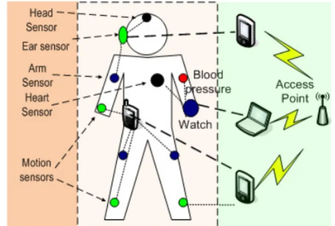
Fig. 1. Wireless body sensor networks. TABLE I
VIDEOSEQUENCE’SPARAMETERS
Ck C1 C2 C3 C4
λk(dB/Kbps) 0.0170 0.0105 0.0064 0.0060
Rk(Kbps) 550 500 400 400
Dk(ms) 350 370 400 420
together with lim
N →∞ W A
2√N D → 0, one can then get
lim inf N →∞ inf²∈[0,1],φ∈[0,2² D][1 − (1 − ²)φA] exp{− W A 2√N D} ≥ 1. Similarly, by Lemma 7, we have
inf²∈[0,1],φ∈[0,2² D][1 − (1 − ²)φA] exp{− W A 2√N D} ≤ 1 − W A 2√N D √ N √ N +2W exp{− W A 2√N D} , ∀N ≥ 1, which together with W λ2(L)
2√N D → 0, when N → ∞ gives lim sup N →∞ inf²∈[0,1],φ∈[0,2² D][1 − (1 − ²)φA] exp{− W A 2√N D} ≤ 1. By Lemma 4 and Lemma 5, we get that
inf (φ,ϕ)∈ΩW r = inf ²∈[0,1](φ,ϕ)∈ΩinfW,² r = inf ²∈[0,1],φ∈[0,2² D] [1 − (1 − ²)φA]. Therefore, we get the result of Theorem 2.
Remark 4 Theorem 2 gives an upper bound of the asymptotic convergence rate under the proposed scheme, and it can be easily extended to other WBSNs with different transmission protocols.
IV. SIMULATIONRESULTS
In this section, we conduct simulations to study the per-formance of the proposed scheduling scheme over a general WBSN platform shown in Fig. 1. There are multiple media flows in this WBSN, and each flow belongs to one of four
0 2 4 6 8 10 2.5 3.0 3.5 4.0 4.5 M O S Time (s) Class# 1 C l a ss# 2 C l a ss# 3 C l a ss# 4
(a) AIMD Method
0 2 4 6 8 10 2.5 3.0 3.5 4.0 4.5 M O S Time (s) Class# 1 C l a ss# 2 C l a ss# 3 C l a ss# 4 (b) Our Method Fig. 2. Average performance comparison based on MOS.
classes (their parameters are listed in Table I). We refer the interested reader to [6] for more details on how these parameters can be extracted. In the simulation, the packet length Lk is 1000 bytes. Link adaptation selects one
appro-priate physical-layer mode depending on the link condition. To demonstrate the effectiveness of our algorithm, we use the Additive-Increase-Multiplicative-Decrease (AIMD)-based rate allocation method [9], which is used by TCP congestion control for comparison.
We test the proposed scheduling in a classic WBSN where nodes may have a constrained communication channel. There are 10 nodes with 0-1 weights, which means that aij = 1
if (i, j) ∈ E, otherwise, aij = 0. The initial states are
chosen as xi(0) = i, i = 1, ..., 10, and Υ = 1.5683. The
control gain is h = 0.75 and the mean of scaling function is W = 0.5. To give a reasonable evaluation for hybrid media flows, we evaluate a concrete quality metric based on MOS (Mean Opinion Score) value. MOS reflects the average user satisfaction on a scale from 1 to 4.5 [4]. The minimum value reflects an unacceptable application quality, and the maximum value refers to an excellent QoS. Fig. 2 presents the average MOS for the 4 flows of different classes obtained by the AIMD method and the proposed method, respectively. It is observed that the proposed method outperforms the AIMD method on the aspect of constant performance. That is because our proposed method manages to keep a rather constant application quality for all active flows by constantly adapting and redistributing the control gain h to all the media flows. Furthermore, the proposed method takes advantage of explicit knowledge of the network characteristics (e.g., Υ, A and D), therefore, it can achieve a better performance than the AIMD method. It should also be noted from Fig. 2(b) that the class with higher priority has higher MOS value than that of lower priority, e.g., the average MOS value of class-1 is 3.9 while that of class-4 is 3.3. This is because the higher priority class usually has higher scheduling priority in the queue of each node to achieve the optimal value of (6).
V. CONCLUSIONS
In this paper, we develop and evaluate a media-aware scheduling scheme over wireless body sensor network by jointly considering constrained communication, node place-ment and transmission latency. We first construct a general flow transmission model according to the network’s trans-mission mechanism, as well as flow’s characteristics. Then, a distributed scheduling scheme is proposed based on dynamic network resource update. It is proved that the proposed scheme can achieve optimal scheduling solution with an exponential convergence rate. The simulation results demonstrate the ef-fectiveness of our proposed scheme.
REFERENCES
[1] M. Chen, S. Gonzalez, A. Vasilakos, H. Cao and V. Leung, “Body Area Networks: A Survey,” ACM/Springer Mobile Networks and Applications, to appear in 2010.
[2] B. P. L. Lo, S. Thiemjarus, R. King, G. Yang, “Body Sensor Network - A Wireless Sensor Platform for Pervasive Healthcare Monitoring,” in Proc. of The 3rd International conference on Pervasive Computing, 2005. [3] A. Barth, S. Wilson, M. Hanson, H. Powell, D. Unluer, J. Lach,
“Body-Coupled Communication for Body Sensor Networks,” in Proc. of The 3rd
International Conference on Body Area Networks, 2008.
[4] L. Zhou, X. Wang, W. Tu, G. Mutean, and B. Geller, “Distributed Scheduling Scheme for Video Streaming over Channel Multi-Radio Multi-Hop Wireless Networks,” IEEE Journal on Selected Areas
in Communications, vol. 28, no. 3, pp. 409-419, Apr. 2010.
[5] E. Farella, A. Pieracci, L. Benini, L. Rocchi, A. Acquaviva, “Interfacing Human and Computer with Wireless Body Area Sensor Networks: the WiMoCA solution,” Multimedia Tools and Applications, vol. 38, no. 3, pp. 337-363, 2008.
[6] H.-P. Shiang, M. Schaar, “Information-Constrained Resource Allocation in Multi-Camera Wireless Surveillance Networks,” IEEE Transactions on
Circuits and Systems for Video Technology, vol. 20, no. 4, pp. 505-517,
2010.
[7] G. P. Davidoff, P. Sarnak and A. Valette, “Elementary Number Theory, Group Theory and Ramanujan Graphs,” London: Cambridge University Press, 2003.
[8] T. Li, M. Fu, L. Xie and J. Zhang, “Distributed Consensus with Limited Communication Data Rate,” IEEE Transactions on Automatic Control, to appear in 2010.
[9] E. Altman, K. Avrachenkov, “Performance analysis of AIMD mechanisms over a multi-state Markovian path”, Computer Networks, vol. 47, no. 3, pp. 307-326, 2005.