HAL Id: hal-01023615
https://hal.archives-ouvertes.fr/hal-01023615
Submitted on 15 Jul 2014
HAL is a multi-disciplinary open access
archive for the deposit and dissemination of
sci-entific research documents, whether they are
pub-lished or not. The documents may come from
teaching and research institutions in France or
abroad, or from public or private research centers.
L’archive ouverte pluridisciplinaire HAL, est
destinée au dépôt et à la diffusion de documents
scientifiques de niveau recherche, publiés ou non,
émanant des établissements d’enseignement et de
recherche français ou étrangers, des laboratoires
publics ou privés.
A Multi-Modal System for Road Detection and
Segmentation
Xiao Hu, Sergio Alberto Rodriguez Florez, Alexander Gepperth
To cite this version:
Xiao Hu, Sergio Alberto Rodriguez Florez, Alexander Gepperth. A Multi-Modal System for Road
Detection and Segmentation. IEEE Intelligent Vehicles Symposium, Jun 2014, Dearborn, Michigan,
United States. pp.1365-1370. �hal-01023615�
A Multi-Modal System for Road Detection and Segmentation
Xiao Hu
1, Sergio A. Rodríguez F.
1,2, Alexander Gepperth
4 Abstract—Reliable road detection is a key issue for modernIntelligent Vehicles, since it can help to identify the driv-able area as well as boosting other perception functions like object detection. However, real environments present several challenges like illumination changes and varying weather conditions. We propose a multi-modal road detection and segmentation method based on monocular images and HD multi-layer LIDAR data (3D point cloud). This algorithm consists of three stages: extraction of ground points from multi-layer LIDAR, transformation of color camera information to an illumination-invariant representation, and lastly the segmentation of the road area. For the first module, the core function is to extract the ground points from LIDAR data. To this end a road boundary detection is performed based on histogram analysis, then a plane estimation using RANSAC, and a ground point extraction according to the point-to-plane distance. In the second module, an image representation of illumination-invariant features is computed simultaneously. Ground points are projected to image plane and then used to compute a road probability map using a Gaussian model. The combination of these modalities improves the robustness of the whole system and reduces the overall computational time, since the first two modules can be run in parallel. Quantitative experiments carried on the public KITTI dataset enhanced by road annotations confirmed the effectiveness of the proposed method.
Keywords—multi-modal perception, monocular vision, LI-DAR, Intelligent Vehicle, road detection
I. INTRODUCTION
Intelligent Vehicles (IV) constitutes a research focus in recent years with promising benefits to society, including the prevention of accidents, optimal transportation planning and fuel conservation [11]. Among various tasks, IV needs to be able to perform road detection which greatly helps for scene understanding as well as boosting object (pedestrian, vehicle) detection functions by restricting the search space. Moreover, road detection could be an alternative solution for departure warning in cases when lane keeping assistance system fails (e.g. less structured roads without well-defined lane markers). However, it remains a complex task since the algorithm should be able to deal with surrounding objects (e.g. vehicles, pedestrian), different environments (e.g. urban, highways, off–road), road types (e.g. shape, color), and sensor exposure conditions (e.g. varying illu-mination, different viewpoints and weather conditions) [2]. Many approaches have been proposed in recent decades, using either passive sensors (e.g. vision), or active ones (e.g. LIDAR and RADAR) [2]. Monocular vision based road detection methods usually rely on features in terms of pixel properties such as intensity [5], color [13], [17] or texture [20], [25], [16], [15] and grouping technologies for
The authors are with1
Université de Technologie de Compiègne (UTC),
2
Université Paris-Sud, Institut d’Eléctronique Fondamentale UMR 8622,
3
Ecole Nationale Superieure de Techniques Avancés, Palaiseau, France
Contact [email protected]
segmentation. Among them, color features receive increasing popularity because of their superiority of representing the world and less physical restrictions. To efficiently deal with illumination changes and shadows, several popular color spaces have been introduced including HSI (Hue, Satura-tion and Intensity) [20], normalized RGB [22] and log-chromaticity space [4]. Stereo vision algorithms not only consider 2D image features but also take advantage of 3D scene information for estimating free space and obstacles using V-Disparity Map techniques [24], [23], [17]. These approaches have improved monocular vision results by the use of a new imaging sensor which grants access to an environment structure prior (i.e. road plane assumption). The variety of sensors opens a large spectrum of possibilities for the use of multiple perception modalities. Multi-modal road detection presented in [6] combines a camera with a LIDAR sensor. [2] propose an interesting method which uses a Geographical Information Systems (GIS) and a GPS receiver to find the corresponding road patch. Later, this information is combined with the image from a monocular camera to obtain the final result.
Hereafter, a multi-modal system is proposed for road detection and segmentation. Two modalities are used, a monocular vision system and an HD multi-layer LIDAR (i.e. Velodyne). The data of both sensors are analyzed by means of three processing stages (see Fig.1). The first stage extracts the ground from 3D laser data providing the environment structure prior. The second, transforms the color image into an illumination-invariant gray scale space. Finally, road image regions are obtained by the combination of pre-computed data in a probabilistic framework. The approach, detailed in this paper, addresses the common need of a road feature initialization step in methods using monocular vision [22], [2], [17], [24], [4]. To this end, the state-of-the-art usually assumes the lower part of the image being the road surface. However, this assumption is not respected under important pitch changes and in scenarios with heavy traffic. The latter situation implies that vehicles are quite close to the field of view of the camera limiting the visibility of the road surface. In contrast, our proposed method determines a potential road surface from 3D laser data and exploits this knowledge to identify image road features.
The remainder of this paper is as follows: First, the framework of the algorithm is outlined in Sect. II. The three main stages introduced previous are detailed consecutively in Sect. III, Sect. IV, Sect. V. Experimental results are demonstrated and discussed in Sect. VI. Finally, conclusions and future work are outlined in Sect. VII.
II. MODALITIES OF THEPERCEPTION SYSTEM
The perception set-up assumed for this study, makes use of a monocular vision system mounted facing forward and an HD multi-layer LIDAR installed on the roof of the
HD Multi-layer LIDAR
RGB Camera Illumination-invariant Image Conversion
RGB space projection into log-chromaticity space
Road Boundary Detection
Identification of the navigable space
Ground Plane Estimation
Ground surface model
Ground Points Extraction
Classification of 3D points lying on the ground surface
Probability Map
Bayesian framework for data fusion
Image Segmentation
Pixel classification using road features
Figure 1: Outline of the multi-modal perception strategy vehicle. Such a system set-up ensures a total inclusion of
the 90° camera’s field of view (FOV) in the HD multi-layer LIDAR range (range up to 120m). Here, we assume the HD multi-layer LIDAR data have been compensated and synchronized with images of the monocular camera as stated in [21]. Extrinsic calibration information between sensors is considered known. The coordinate system of the HD multi-layer LIDAR is denoted L and its corresponding axes XL,
YL and ZL. The monocular camera is represented through a pinhole projective model with no distortion and zero skew. Its frame,C, and axes, XC, YC and ZC are illustrated in Fig.
2. Forward Left HD Multi-layer lidar Camera HD multi-layer es XL, multi-layer , YL LIDAR and ZL. model XC, model with , YC no distortion and ZC
HD Multi-layer lidar FOV Camera FOV
Figure 2: Coordinate systems for HD multi-layer lidar and camera.
III. GROUND PLANE DETECTION USINGHD
MULTI-LAYERLIDAR
As introduced previously, the first module takes the LI-DAR point cloud as input and outputs ground points. There are three main sub-functions: (III-A) road boundary detec-tion, (III-B), candidates selection and plane estimation(III-C) and ground points extraction according to the point-to-plane distance. Note that the proposed ground points extraction method is based on the detection of the road boundaries, which are assumed to exist.
A. Road Boundary Detection
Road boundary information is useful for road detection, e.g., to define road curvature. For a typical 2D vision system, this task is usually addressed by edge detection. For LIDAR sensors, a fast and simple method for curb detection relying on LIDAR scan histograms was proposed in [8]. LIDAR points are projected to 2D plane (i.e. XL− YL plane), and
a histogram is built along the axis orthogonal to the driving direction. It is easy to understand that a large number of LIDAR points will be accumulated on the road boundaries, producing two peaks in the histogram (see upper row in Fig. 3). However, this method is prone to fail in steering and roundabout scenarios as stated in [19] because the histogram may fade out (see lower row in Fig. 3). Here, temporal filtering is used to overcome difficulties in such situations.
Figure 3: Road boundary detection based on histograms: the upper figure is the histogram when the vehicle runs almost straight; the lower figure is the histogram when the vehicle is steering.
B. Plane Estimation
In order to identify 3D LIDAR candidate points, we assume that road boundaries always “stand” on the road plane. That is to say, if the boundary is projected to the ZL axis (Fig.2), the points with the smallest values along
the ZL axis are assumed to be close to the road plane (i.e. small pitch angles). Based on this assumption, a cell-based candidate selection process is performed for all boundary points. First, points are clustered into different cells of size δcell, according to their XL coordinate. Then for each cell,
the point with the lowest elevation in LIDAR frame (Fig.2) is selected and added to a list, see Fig. 4 as an example. Finally, the ground plane in 3D space is determined by fitting the obtained list of points to the model:
axL+ byL+ czL+ d = 0 (1)
with a, b, c, d being the plane parameters. The RANSAC algorithm is used here for robust plane parameters esti-mation. Compared to considering all LIDAR points, this method reduces the probability of outliers and results in a better and faster estimation.
C. Ground Points Extraction
Once the road plane has been estimated, the orthogonal distance between any 3D point and the plane is computed. Based on this criterion, ground points are extracted through a thresholding procedure. Let disibe the orthogonal distance
Figure 4: Assumption and candidates selection procedure.
disi=
axLi + byiL+ cziL+ d
p
a2+ b2+ c2 (2)
and the set of 3D points lying on the ground plane selected by the following criterion:
pi, t = ⇢ pg, t, if|disi| < disthr png, t, otherwise ◆ , i= 1 · · · Np, t (3)
where, pi, t denotes the ith 3D point, pg, t and png, t
correspond to ground and non-ground point class labels, respectively. disthris a threshold which is manually set (e.g.
typically 0.15m) and Np, t stands for the total number of
3D scan points at time t. This technique may fail, which usually implies an radical decrease of the number of ground points, Ng, t−1. In that case, even if the selection procedure
is already taken, many points are still far from the real ground plane (see Fig. 5). The estimated plane is not reliable as it is illustrated in the blue zone in the left image of Fig. 6). To cope with this problem, a short-term memory approach [20], [26] is employed as follows:
Let t be the current index time. Then, the ground points at t− 1, Pt−1, are memorized and predicted, Pt|t−1, by the
means of a constant speed evolution model: xL t = xLt−1− vx⇤ Te yLt = ytL−1− vy⇤ Te zL t = ztL−1− vz⇤ Te (4)
where xLt, ytL, ztLare the point coordinates at time t in theL
frame, xt−1, yt−1, zt−1are point coordinates at time t−1 in
L frame, vx, vy, vzare the speed vector components of host
vehicle. Te is the period. 3D points beyond a certain range
(typically around 60m ground plane assumption remains meaningful) are discarded.
Figure 5: Projection of selected candidates into the RGB image. The right figure shows an example case where ground plane classification fails.
The 3D scan points Pt|t−1 predicted using the evolution
model stated in Eq. III-C, are kept if Ng, t⌧ Ng, t|t−1where
Ng, t and Ng, t|t−1 are respectively the cardinalities of the
sets Pt and Pt|t−1. That is to say, the cardinality of the
ground point set should not change too fast over time given the frequency of HD multi-layer lidar (10 Hz) and the fact that vehicle always runs on the road. The classified points
result affected by road side
objects improved result
Figure 6: Results of the same frame without (left) and with (right) Short-Memory Technology.
are then replaced by the predicted ones in current frame (see Fig. 6).
This method can roughly detect ground points regardless of any objects that may be close to the vehicle. The ground points set includes 3D points lying on the road plane and other low-rise obstacles.
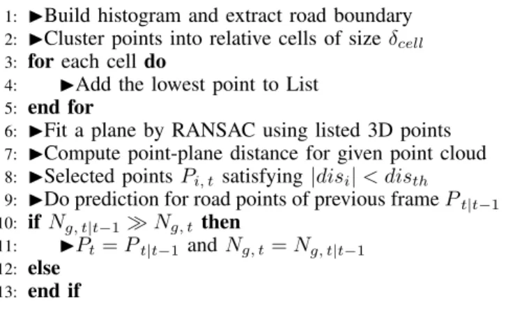
D. Ground point classification algorithm Algorithm III.1
Input: - 3D point cloud from HD multi-layer LIDAR Output: - Ground points
1: IBuild histogram and extract road boundary
2: ICluster points into relative cells of size δcell
3: for each cell do
4: IAdd the lowest point to List
5: end for
6: IFit a plane by RANSAC using listed 3D points
7: ICompute point-plane distance for given point cloud
8: ISelected points Pi, t satisfying|disi| < disth
9: IDo prediction for road points of previous frame Pt|t−1
10: ifNg, t|t−1% Ng, t then
11: IPt= Pt|t−1 and Ng, t= Ng, t|t−1
12: else
13: end if
IV. IMAGE SPACE TRANSFORMATION
In the second module, the color image is transformed to a representation that is robust to shadow and illumination changes simultaneously.
A. Illumination-Invariant Image Tranformation
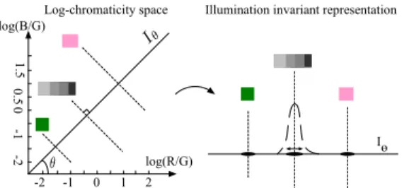
RGB color images are usually transformed to other color spaces (e.g., HSI [20], log-chromaticity space [4]) in order to obtain features that are independent of shadows and lighting condition. In this module, the log-chromaticity space widely used [24], [7] is applied. [9] pointed that an illuminant-invariant image Iθcould be generated given the assumptions
of Lambertian surfaces and Planckian light sources, which was extented to approximately suitable conditions by [4]. In the log-chromaticity space (Fig. 7) defined by the two axes {log(R
G), log( B
G)}, color surfaces of different chromaticities
are represented by parallel lines and the same color surface at different illuminations is located on a single straight line. By projecting the values of the log-chromaticity space along an orthogonal axis defined with an angle θ to the horizontal axis, a grayscale image Iθ can be obtained. θ depends on
-2 -1 0 1 2 log(R/G) log(B/G) 1.5 0.5 0 -1 Iɵ -2 indicating(Iθx,y (Iθ
Log-chromaticity space Illumination invariant representation
Figure 7: Log-chromaticity space and the corresponding illumination invariant representation.
V. PROBABILISTIC FRAMEWORK FORIMAGE-LIDAR
DATA COMBINATION
The third module serves as the fusion center where the projection of ground points and the gray image are fused to compute a Gaussian model as well as a probability map. Road areas are finally classified and segmented.
A. Probability Map
A similar probability map is generated here for road classification and segmentation to that of [3], [1]. The larger the probability is, the more likely the pixel belongs to the road class. The image is divided into two classes for computing the probability: sky area and non-sky area. Pixels of sky area cannot be road pixels, i.e., the corresponding probability should be 0. This could also be seen as a sky removal procedure. For pixels within the non-sky area, a parametric model based on Gaussian functions is used for computing the probabilities, see Sec. V-A2.
1) Sky Removal: The horizon line is used here to classify the sky and non-sky area: any area over the horizon line is considered sky area and vice versa. Regard to the estimation of horizon line, a straightforward method inspired by [14] is used here, where a virtual point, denoted P1, which lies on
the ground plane and is 2000 meters away from the LIDAR sensor is created (Eq.5) under the assumption that the camera height is identical to the height of the LIDAR sensor. After projection to the camera frame C, the corresponding pixel, denoted as pixel1, should be close to the horizon line.
Based on this ideal, the horizon line can be easily estimated. The probabilities of pixels above the horizon line are set to 0. P1= (2000, 0, −h) with h = 1 Ng, t Ng, t X i=1 ZiL (5) pixel1= MCL· P1 (6) where, MC
L represents the 4 ⇥ 4 transformation matrix
from the LIDAR frame to the camera frame (Fig.2). All coordinates are expressed using homogeneous representation for easy computation.
2) Parametric Gaussian Model: The subsequent calcu-lations make use of the illuminant-invariant image in log-chromaticity in subsection IV-A and Fig. 7. Road pixels corresponding to the points in log-chromaticity space should be very close. After projection to the axis defined by θ, their distribution should be within a narrow band due to various noises. A parametric Gaussian function model (defined with mean value µ and variance σ2) is used here
for representing the distribution. The pre-computed ground points are projected into the camera frame and then used as a representative training data for computing the Gaussian parameters µ and σ2. As this model is computed frame
by frame and the ground points are located in different patches of the road, it can adapt to varying environments and conditions (e.g. shadow covers part of the road). At this point, it is possible to score all pixels of the non-sky area according to the parametric models. Individual pixels are assigned a score by passing its illumination-invariant feature value through a Gaussian using the learned parameters. The output is a pixel–wise map indicating similarity to the road model and is obtained by:
probx,y = exp(−
(Iθx,y− µ)2
2σ2 ) (7)
where, x and y are the pixel coordinates. B. Classification and Segmentation
The model-based classification [24], [4], [18] is applied to the probability map for road pixel identification as fol-lows:
pixel= ⇢
road if probi> Tλ
non-road otherwise (8) where Tλ is a threshold set so as to keep the most
probable road pixels.
After classification, a connected-components segmenta-tion is operated with road pixels serving as seeds. In order to cope with probability map errors and to remove outliers lay closely to road area, e.g., points on the grassland, we only select the patch with the most road pixels included as the proper road region. Finally, a flood-fill algorithm is applied for filling small holes.
C. Summary
Algorithm V.2 Multimodal Road Detection Algorithm Input: - Point cloud;
- Color Image;
Output: - Road identified image;
1: I Run Ground Points Extraction algorithm and get ground points
2: ITransform color image to illuminant-invariant image
3: I Project ground points to image and initialize the ground pixels
4: IBuild the parametric model using ground pixels
5: ICompute probability map
6: IClassification using thresholding
7: IRun component-connect algorithm
8: ISelect the component with the maximum number of ground pixels
9: IRun flood fill algorithm to fill the holes
VI. EXPERIMENTS
To evaluate the performance of the proposed approach, the database of the KITTI [12] Vision Benchmark Suite is used. The KITTI dataset is collected in real-world scenes, e.g., city, road, residential area. In addition, a comparison is made between the proposed method and the traditional histogram based approach. The test system includes: a
computer with Pentium 3200 processor and 3 GB memory running a Linux operating system. The program is currently implemented in MATLAB.
A. Results
The tests that were carried include different samples with the presence of nearby objects and high saturation. Some of them may be viewed in column (a) of Fig 8.
The parameters of the proposed method were set as follows: size of cell δcell for candidates selection: 0.15m;
the threshold disthr for ground points extraction: 0.15m;
the invariant direction θ for illumination-invariant image transformation:45◦
; the threshold Tλfor road classification:
0.68. Tλ is set by learning.
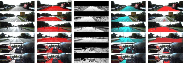
The performance of the proposed method is validated and compared to the road detection algorithm in [4]. Example results are shown in Fig 8. In these images, road areas are painted to cyan color. The two right-most columns show the differences between the proposed method and the method in [4]. As expected, the method in [4] fails in some situations because its assumption about the initial seed zone does not hold. For example, when seeds are all located on a lane marking, a failure occurs which is also mentioned in [4]. In this case, the histogram used for classification can only be a representative of lane marking instead of the road area as a whole. Another instance is shown in Fig 8, where seeds are selected from an object and not from the true road area. In contrast, the proposed method works well in these scenarios since it does not rely on the initial guess of seeds. Even in hard scenarios of heavy traffic, it is possible to acquire good estimations of road area rather than false detections. More results in streaming video format can be accessed1. The algorithm implemented in MATLAB code requires around 600 ms processing time per frame (size of 1242 × 375), so a C++ implementation can be expected to achieve real-time capability, with additional speed-ups possible through the parallelization of the first two modules which do not depend upon each other.
Nevertheless, the proposed method encounters failures. The analysis of failures reveals two main reasons: 1) in some frames, the roof of a observed car is misdetected because it looks almost white which is quite similar to the remote road pixels under oversaturated illumination. The two classes are very difficult to discriminate. The same problem of illumination-invariant features under extreme saturation is also mentioned in [1], [4]. Improvements may be obtained by improving the acquisition system [4] or an additional pass of comparison to LIDAR points. 2) ground points are misdetected in some conditions where no road boundary can be found. This can be addressed by improving the ground points extraction.
B. Quantitative Evaluation
Quantitative evaluation is performed on the UMM dataset detailed in [10]. UMM dataset consists of 95 images selected from several different videos. All these images are manually segmented to generate the ground truth. Perfor-mance evaluation is provided using pixel-wise measures
1https://www.youtube.com/watch?v=B7pwyyxDCj4
Table I: Pixel-wise measures used to evaluate the perfor-mance of the detection results.
Pixel-wise measure Definition
Precision T P
T P +F P
Recall T P
T P +F N
F1-measure 2Precision Recall
Precision+Recall
Fmax argmax
τ
(F1-measure)
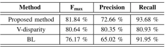
Table II: Performance evaluation on KITTI-UMM dataset.
Method Fmax Precision Recall
Proposed method 81.84 % 72.66 % 93.68 %
V-disparity 80.64 % 80.35 % 80.93 %
BL 76.17 % 65.02 % 91.95 %
defined in Table I: where T P is the number of correctly labeled road pixels, F P is number of non-road pixels erroneously labeled as road and F N is the number of road pixels erroneously marked as non-road. Precision and Recall provide different insights in the performance of the method: Low precision means that many background pixels are classified as road, whereas low recall indicates failure to detect the road surface. Finally, F1-measure (or effective-ness) is the tradeoff using weighted harmonic mean between precision and recall [1]. The maximum F1-measure is used here for comparison by varying the classification threshold τ (corresponds to Tλ in the proposed method), yielding Fmax.
All three measures range from 0 to 1, and higher values are desired. The performance of the proposed method is validated and compared to state-of-the-art algorithms based on a similar illumination-invariant feature and V-disparity [24]. For fair comparison, we used the program provided by the authors and keep their parameter settings since their parameters were learnt from the same dataset. The baseline (BL) detailed in [10] is also added for comparison. Note that since the images are extracted from different videos and consequently isolated, the short-memory technology of our method is shut down. A summary of results is listed in Table II. As shown, the proposed method outperforms the V-disparity based method and baseline in terms of Fmaxand
recall. However, the proposed method has a lower precision, which means that there are many false detections in the proposed method. The reason for this phenomenon is the failure of the ground points detection method in some cases as explained in the previous section.
VII. CONCLUSION ANDFUTUREWORK
In this paper, a novel multi-modal based road detection approach has been presented. The approach can be divided into three modules with the first two modules can run in parallel. Ground points are extracted in the first mod-ule while an illumination-invariant feature representation is computed simultaneously in the second module. Through the registration, they are fused in the third module through a parametric model for building a probability map. Final classification and segmentation of road area is done by applying basic segmentation and region growing algorithms to this map. Experiments are performed on a public data set in order to validate the proposed method. Furthermore, the algorithm is compared with one state-of-the-art methods in a qualitative way. From the experimental results, the proposed
(a) (b) (c) (d) (e)
Figure 8: Experimental Results: from left to right, (a) The original image. (b) The projection of ground points. (c) The probability map. (d) Road detection result of the proposed method. (e) Road detection result by [4] .
method demonstrates its efficiency of extracting road area from the image under different and severe conditions where state-of-the-art methods may fail.
As future work, the real-time implementation will be achieved by programming in C++, code optimization and parallel computing. More robust ground points extraction methods and multiple Gaussian models will also be tested.
ACKNOWLEDGMENTS
This project was financed and supported by University Paris-Sud.
REFERENCES
[1] J.M. Alvarez, T. Gevers, and A.M. Lopez. 3d scene priors for road detection. In Computer Vision and Pattern Recognition (CVPR), IEEE Conference on, pages 57–64, 2010.
[2] J.M. Alvarez, F. Lumbreras, T. Gevers, and A.M. Lopez. Geographic information for vision-based road detection. In Intelligent Vehicles Symposium (IV), IEEE, pages 621–626, 2010.
[3] J.M.A. Alvarez, T. Gevers, and A.M. Lopez. Vision-based road detection using road models. In Image Processing (ICIP), 16th IEEE International Conference on, pages 2073–2076, 2009.
[4] J.M.A. Alvarez and A.M. Lopez. Road detection based on illuminant invariance. Intelligent Transportation Systems, IEEE Transactions on, 12(1):184–193, 2011.
[5] Alberto Broggi and Simona Berte. Vision-based road detection in automotive systems: A real-time expectation-driven approach. Journal of Artificial Intelligence Research, pages 325–348, 1995. [6] H. Dahlkamp, A. Kaehler, D. Stavens, S. Thrun, and G. Bradski.
Self-supervised monocular road detection in desert terrain. In Proceedings of Robotics: Science and Systems, 2006.
[7] F. Diego, J.M.A. Alvarez, J. Serrat, and A.M. Lopez. Vision-based road detection via on-line video registration. In Intelligent Transportation Systems, 13th International IEEE Conference on, pages 1135–1140, 2010.
[8] Fadi Fayad and Veronique Cherfaoui. Tracking objects using a laser scanner in driving situation based on modeling target shape. In Intelligent Vehicles Symposium, IEEE, pages 44–49, 2007. [9] G.D. Finlayson, S.D. Hordley, Cheng Lu, and M.S. Drew. On the
removal of shadows from images. Pattern Analysis and Machine Intelligence, IEEE Transactions on, 28(1):59–68, 2006.
[10] Jannik Fritsch, Tobias Kuehnl, and Andreas Geiger. A new per-formance measure and evaluation benchmark for road detection algorithms. In Intelligent Transportation Systems, 16th International IEEE Conference on, 2013.
[11] Andreas Geiger. Probabilistic Models for 3D Urban Scene Under-standing from Movable Platforms. PhD thesis, 2013.
[12] Andreas Geiger, Philip Lenz, Christoph Stiller, and Raquel Urtasun. Vision meets robotics: The kitti dataset. International Journal of Robotics Research (IJRR), 2013.
[13] Yinghua He, Hong Wang, and Bo Zhang. Color-based road detection in urban traffic scenes. Intelligent Transportation Systems, IEEE Transactions on, 5(4):309–318, 2004.
[14] D. Held, J. Levinson, and S. Thrun. A probabilistic framework for car detection in images using context and scale. In Robotics and Automation (ICRA), IEEE International Conference on, pages 1628– 1634, 2012.
[15] Hui Kong, J-Y Audibert, and Jean Ponce. General road detection from a single image. Image Processing, IEEE Transactions on, 19(8):2211–2220, 2010.
[16] P. Lombardi, M. Zanin, and S. Messelodi. Switching models for vision-based on-board road detection. In Intelligent Transportation Systems, Proceedings, pages 67–72. IEEE, 2005.
[17] A. Miranda Neto, A. Correa Victorino, I. Fantoni, and J.V. Ferreira. Real-time estimation of drivable image area based on monocular vision. In Intelligent Vehicles Symposium (IV), pages 63–68. IEEE, 2013.
[18] A. Petrovskaya and S. Thrun. Model based vehicle tracking for autonomous driving in urban environments. In Proc. of Robotics: Science and Systems, Zurich, Switzerland, June 2008.
[19] Sergio A. Rodriguez. Contributions by Vision Systems to Multi-sensor Object Localization and Tracking for Intelligent Vehicles. PhD thesis, Universite de Technologie de Compiegne, 2010.
[20] M. Sotelo, F. Rodriguez, L. Magdalena, L. Bergasa, and L. Boquete. A color vision-based lane tracking system for autonomous driving on unmarked roads. Autonomous Robots, 16(1):95–116, 2004. [21] Dominik Steinhauser, Oliver Ruepp, and Darius Burschka. Motion
segmentation and scene classification from 3d lidar data. In Intelli-gent Vehicles Symposium, 2008 IEEE, pages 398–403. IEEE, 2008. [22] C. Tan, Tsai Hong, T. Chang, and M. Shneier. Color model-based real-time learning for road following. In Intelligent Transportation Systems Conference, pages 939–944. IEEE, 2006.
[23] G.B. Vitor, D.A. Lima, A.C. Victorino, and J.V. Ferreira. A 2d/3d vision based approach applied to road detection in urban environments. In Intelligent Vehicles Symposium (IV), pages 952– 957. IEEE, 2013.
[24] Bihao Wang and V. Fremont. Fast road detection from color images. In Intelligent Vehicles Symposium (IV), pages 1209–1214. IEEE, 2013.
[25] K. Yamaguchi, A. Watanabe, T. Naito, and Y. Ninomiya. Road region estimation using a sequence of monocular images. In 19th International Conference on Pattern Recognition, pages 1 –4, dec. 2008.
[26] Gangqiang Zhao and Junsong Yuan. Curb detection and tracking using 3d-lidar scanner. In Image Processing (ICIP), 19th IEEE International Conference on, pages 437–440, 2012.