HAL Id: hal-00984068
https://hal.archives-ouvertes.fr/hal-00984068
Submitted on 27 Apr 2014
HAL is a multi-disciplinary open access
archive for the deposit and dissemination of
sci-entific research documents, whether they are
pub-lished or not. The documents may come from
teaching and research institutions in France or
abroad, or from public or private research centers.
L’archive ouverte pluridisciplinaire HAL, est
destinée au dépôt et à la diffusion de documents
scientifiques de niveau recherche, publiés ou non,
émanant des établissements d’enseignement et de
recherche français ou étrangers, des laboratoires
publics ou privés.
Calibration-Free BCI Based Control
Jonathan Grizou, Iñaki Iturrate, Luis Montesano, Pierre-Yves Oudeyer,
Manuel Lopes
To cite this version:
Jonathan Grizou, Iñaki Iturrate, Luis Montesano, Pierre-Yves Oudeyer, Manuel Lopes.
Calibration-Free BCI Based Control. Twenty-Eighth AAAI Conference on Artificial Intelligence, Jul 2014, Quebec,
Canada. pp.1-8. �hal-00984068�
Calibration-Free BCI Based Control
Jonathan Grizou
Inria Bordeaux Sud-Ouest, France [email protected]
I ˜naki Iturrate
CNBI, EPFL, Switzerland [email protected]
Luis Montesano
I3A, Univ. of Zaragoza, Spain [email protected]
Pierre-Yves Oudeyer
Inria Bordeaux Sud-Ouest, France [email protected]
Manuel Lopes
Inria Bordeaux Sud-Ouest, France [email protected]
Abstract
Recent works have explored the use of brain signals to directly control virtual and robotic agents in sequential tasks. So far in such brain-computer interfaces (BCI), an explicit calibration phase was required to build a de-coder that translates raw electroencephalography (EEG) signals from the brain of each user into meaningful in-structions. This paper proposes a method that removes the calibration phase, and allows a user to control an agent to solve a sequential task. The proposed method assumes a distribution of possible tasks, and infers the interpretation of EEG signals and the task by selecting the hypothesis which best explains the history of inter-action. We introduce a measure of uncertainty on the task and on the EEG signal interpretation to act as an exploratory bonus for a planning strategy. This speeds up learning by guiding the system to regions that better disambiguate among task hypotheses. We report exper-iments where four users use BCI to control an agent on a virtual world to reach a target without any previous calibration process.
Introduction
EEG-based brain-computer interfaces (BCI) have been used successfully to control different devices, such as robotic arms and simulated agents, using self-generated (e.g. motor imagery) and event-related potentials signals (see (Mill´an et al. 2010) for a review). Error-related potentials (ErrPs) are one kind of event-related potential appearing when the user’s expectation diverges from the actual outcome (Falkenstein et al. 2000). Recently, they have been used as feedback instruc-tions for devices to solve a user’s intended task (Chavarriaga and Mill´an 2010; Iturrate, Montesano, and Minguez 2013a). As in most BCI applications, ErrP-based BCI requires a calibration phase to learn a decoder (e.g. a classifier) that translates raw EEG signals from the brain of each user into meaningful instructions. This calibration is required due to specific characteristics of the EEG signals: non-stationary nature (Vidaurre et al. 2011), large intra- and inter-subject variability (Polich 1997), and variations induced by the task (Iturrate, Montesano, and Minguez 2013b). The presence of an explicit calibration phase, whose length and frequency is
Copyright c! 2014, Association for the Advancement of Artificial
Intelligence (www.aaai.org). All rights reserved.
hard to tune and is often tedious and impractical for users, hinders the deployments of BCI applications out of the lab. Thus, calibration free methods are an important step to apply this technology in real applications (Mill´an et al. 2010).
Despite the importance of calibration-free BCI, there are only few related works. For long term operation using sensory-motor rhythms, it is possible to adapt the decoder online (Vidaurre and Blankertz 2010). In invasive BCI, Ors-born et al. (2012) proposed a method to learn from scratch and in closed loop a decoder for known targets using pre-defined policies to each target. However, the approach needs a warm-up period of around 15 minutes. For P300 spellers, Kindermans et al. proposed a method to auto-calibrate the decoder by exploiting multiple stimulations and prior in-formation (Kindermans, Verstraeten, and Schrauwen 2012; Kindermans et al. 2012; Tangermann et al. 2013). They ex-ploit the particular fact that only one event out of six encodes a P300 potential in the speller paradigm.
Our main contribution is a calibration-free BCI method that infers simultaneously and seamlessly an EEG decoder of error-related potentials while controlling a device to achieve a sequential task. The core idea of the method is to assume a distribution of possible tasks, and infer the in-terpretation of EEG signals and the task by selecting the hy-pothesis which best explains the history of interaction. This inference can be continuously run and updated as new data comes in, which removes the need for an explicit calibration. This method is inspired from our previous work (Grizou, Lopes, and Oudeyer 2013) which considered a robotic set-ting and speech utterances as feedback signals. In the current work we improve the algorithm formalism, the robustness to noisy high-dimensional signals (e.g. EEG), and show that it is possible to use model-based planning relying on the un-certainty about the task and the feedback signals interpreta-tion to explore the space efficiently while learning.
We also present an evaluation of this method with online experiments where four users control an agent in a virtual world. The results show that the proposed method allows to learn a good signal decoder and solve the task efficiently without any explicit calibration. Offline experiments show that our unsupervised trained decoder achieves similar per-formances than calibration based systems and illustrate the benefits of our planning strategy for speeding up learning.
Calibration-Free BCI Based Control
BCI control based on feedback signals
BCI control based on feedback signals differs from classical brain-computer interfaces in the sense that the user does not actively deliver commands to the device, but only delivers feedback about actions performed by the device (Chavar-riaga and Mill´an 2010; Iturrate, Montesano, and Minguez 2013a). In this setting, the device needs to actively execute a sequence of several actions to solve the task and to be able to learn an intelligent behavior from the feedback. This idea can be seen as a shared control strategy (Mill´an et al. 2010), where both the user and the device help each other to solve a task.
Essentially, this BCI control follows an iterative sequen-tial process where the device performs an action which is in turn assessed by the user. This assessment will elicit poten-tials into the user’s brain that can be recorded using EEG and will be different for “correct” and “wrong” assessments. The potentials elicited in the user’s brain after performing assess-ments are called error-related potentials (Ferrez and Mill´an 2008). After a calibration phase and once a usable decoder of these signals is available, user’s assessments can be trans-lated into (normally binary) feedback, which the device can use to adapt its behavior.
This control based on user’s assessments decoded from brain signals can be exemplified for a reaching task, where the user wants to reach a target position unknown by the system. The device performs several discrete actions (e.g. moving left or right), and learns from the feedback given by the user. After several iterations, if the meanings of the EEG assessment signals provided by the users are known, the de-vice can infer which is the user’s desired position and how to reach it. The following section explains how we can achieve similar performances without knowing the brain signal de-coder beforehand. We will use the term “virtual label” or “label” to denote the interpretation of a given EEG signal as a feedback instruction (e.g. “correct” or “wrong”).
Simultaneous Estimation of Task and Signal Model
This section formalizes the problem of executing a task when the mapping between raw EEG signals to a discrete la-bel among a set of pre-defined lala-bels is unknown. The main idea is depicted in Figure 1 for a toy 1D example. The user wants the device to reach the right-most state. For each de-vice’s action, he provides a feedback signal which encode whether the action executed is “correct” or “wrong” accord-ing to the intended target. Such signals are generated from an underlying model which maps a binary label (“correct” or “wrong”) to a continuous signal. However, neither the user’s desired target nor the labels associated to the user’s feedback signals are known.
Considering that we can define a finite set of task hypothe-ses (e.g. reaching one of a finite number of states), we can in-fer the labels that should be provided by the user with respect to each hypothesis. Then, given a particular interaction his-tory, it is possible to compute a different signal decoder for each task hypothesis. The key point is that only the correct hypothesis will assign the correct labels to all feedback
sig-T (a) T (b) Class0 Class1 T (c)
Figure 1: Representation of inferred signal labels for a 1D grid world in function of the hypothesized task. Three task hypotheses are displayed in column from left to right [(a), (b), (c)]. On top is a 1D grid world with the hypothetic target state marked with a T letter. Notice that this hypo-thetic target is different for each of the three hypotheses. The arrows in each cell indicates what action should elicit a positive feedback, i.e. the optimal policy with respect to the hypothetic target. The user intended target is shown as the shaded blue state at the right extremity of the 1D world. Note that the system does not have access to this information. The correct hypothesis is the one on the Left [(a)] where the T state is the same as the shaded blue state. Below the 1D grid world, the signals received from the user are represented in a 2D feature space. They represent the user assessment sig-nals of the past history of device’s actions (e.g. moving ran-domly left and right). Our algorithm assigns virtual labels (green for “correct” and red for “wrong”) to those signals with respect to their respective hypothetic target. Notice that the data points are the same for all three hypotheses, only their respective labels differ. With the virtual labels being assigned, we can compute the corresponding 2D Gaussian distributions estimates for each class (shown as colored el-lipses) and each hypothesis. While for the correct hypothe-sis [(a)] the Gaussian distributions shows a large separabil-ity, the overlap increases as the hypothetic target (T) moves away from the real (blue shaded) one [(b), (c)]. This prop-erty can be exploited to estimate the correct hypothesis and the model generating the signals.
nals (Figure 1a), while the other hypotheses will gradually mix both classes as the hypothetic target gradually differs more from the correct one (Figure 1b and 1c). Therefore, the hypothesis which provides the decoder with best accu-racy and compactness can be selected as the most probable one. In the remainder of this section we show how this prop-erty can be exploited to estimate the target and the model generating the feedback signals.
Formally, we represent the problem as a discrete or con-tinuous set of states s 2 S, a finite set of possible actions a2 A, and a set of possible tasks, or targets, for which the system is able to plan the best sequence of actions. In the 1D example in Figure 1, the state space is composed of seven discrete states, and the agent can perform unitary directional actions, i.e. move one cell left or right. During an interactive learning session, the agent will proactively perform actions which will in turn be evaluated as “correct” or “wrong” by the user with respect to the desired target state on the grid. In our case the feedback signals are error-related potentials measured in the brain activity of the subject.
Let ei 2 Rn denote the feature vector of the EEG
mea-surements obtained at iteration i after the device performed action aiin state si. The label zi2 {c, w} of each feedback
signal belongs to one of two classes (“correct” or “wrong”). Following Blankertz et al. (2010), we will model the EEG signals using independent multivariate normal distributions for each class (N (µc,Σc) and N (µw,Σw)). We will denote
by θ this set of parameters{µc,Σc, µw,Σw}.
We assume the system has access to a set of task hypothe-ses ξ1, . . . , ξT which includes the task the user wants to
solve. We do not make any particular assumption on how the task is represented but we assume that for each par-ticular task ξ we are able to compute a policy πξ which
represents the probability of choosing a given action a in state s, πξ(s, a) = p(a|s, ξ). As mentioned above, these
are the policies that, conditioned on the task, provide la-bels to the feedback signals of a state-action pair (e.g. in a reaching task, progressing towards the goal will generate “correct” feedback while moving apart from it will generate “wrong”feedback).
The method aims to infer which task ˆξ the user wants to solve based on the user’s feedback signals extracted from EEG measurements collected while the agent executes some actions. Following the analysis of Figure 1, a sensible option to estimate the task is to measure the coherence of the sig-nal model for each possible task using the virtual labels pro-vided by the target policy. In other words, the best(ξ, θ) pair provides the lowest predictive error on the observed signals p(e|s, a, ξ, θ), which themselves were collected in the recent history of interaction. One possible way of solving this prob-lem is to maximize the expected classification rate:
ˆ
ξ, ˆθ = arg max
ξ,θ Ee[δ(z(s, a, ξ), z(e, θ))] (1)
where δ() is an indicator function, z(s, a, ξ) is the label (cor-rect or wrong) corresponding to the execution of action a in state s under task ξ and z(e, θ) is the label provided by classifying the EEG signal e under the Gaussian classifier parameterized by θ. The expected classification rate (Ecr) can be explicitly written dependent on the task and decoder model:
Ecr(δ(z(s, a, ξ), z(e, θ))) =
= X
k∈{c,w}
p(z = k|s, a, ξ)p(z = k|e, θ) (2)
where p(z = k|s, a, ξ) represents the probability of the user assigning label k when assessing action a in state s accord-ing to task ξ. We add a noise term to cope with those situa-tions where the user assessment may be wrong. The model for probability of correct assessment is then:
p(z = c|s, a, ξ) =⇢1 − α if a = arg maxaπξ(s, a) α otherwise
(3) with α modeling the assessment error rate of the user, which was set to0.1 for our experiments. Finally, the term p(z = k|e, θ) is just the probability that the signal e belong to class
k under the Gaussian model provided by θ and is given by: p(z = k|e, θ) = P p(e|z = k, θ)p(z = k)
l∈{c,w}p(e|z = l, θ)p(z = l)
= P N (e|µk,Σk)p(z = k)
l∈{c,w}N (e|µl,Σl)p(z = l)
(4) As we do not have a priori knowledge on the user intended meaning, we assume that it is equiprobable p(z = c) = p(z = w). We will factorize the optimization process using the fact that given a task ξ, the estimation of θ under the Gaussian model is straightforward. It basically requires to compute the maximum-likelihood estimate θM L
ξ using the
labels associated to target ξ. We could also consider a prior distribution on the parameters and update it with new ob-servations. Using the labels of target ξ, the estimation of θ under the Gaussian model described above simply returns to the computation of the posterior mean µzand covariance
Σz for each class z 2 {c, w}. In order to avoid numerical
problems when estimating the covariance for a low number of examples, a regularization term was applied to penalize very large and very small eigenvalues (Friedman 1989):
Σz= (1 − λ)Σz+ λ
trace(Σz)
n In (5)
with n the feature dimension, Inthe identity matrix of size
n, and λ the regularization term which was set to0.5 for our experiments. An automatic adaptation of the regularization could also be considered (Ledoit and Wolf 2004).
Using equation 2 to estimate the expected classification rate is difficult because we ideally want to estimate it on future, never observed, data. A possible solution is to use cross-validation or bootstrapping methods using the avail-able data. However, for small amounts of data, these meth-ods result in estimates with high variance (Bengio and Grandvalet 2004) and computational cost.
Alternatively, we propose to use another approximation of the expected classification rate, the Bhattacharyya co-efficient. This coefficient has been related to the classi-fication error of Gaussian models (Kailath 1967) and is inversely proportional to the classification rate. Although there is no analytical relation between the coefficient and the classification rate, it is possible to derive bounds and good empirical approximations (Lee and Choi 2000). The Bhattacharyya coefficient ρ 2 [0, 1] between the Gaussian distributions associated to label “correct” (N (µc,Σc)) and
“wrong” (N (µw,Σw)) is:
ρ= e−DB(θ)
(6) where DBis the Bhattacharyya distance: DB(θ) =
1 8(µc− µw)T(Σc+Σ2 w)−1(µc− µw) +12ln ⇣ det(Σc +Σw 2 ) √ detΣcdetΣw ⌘ . Finally, we approximate the expected classification rate as:
Ecr/ 1 − ρ (7)
Confidence on Target Estimation
Now that we have an estimation of the expected classifica-tion rate, we need to take a decision with respect to which
task is the one intended by the user. To do so we should com-pare the expected classification rate of every task hypothesis ξtwith t 2 {1, . . . , T }. The hypothesis whose associated
model has the highest expected classification rate, i.e. the lowest value of ρ, is expected to be the one intended by the user, however it is meaningless to define an absolute thresh-old on the value of the expected classification rate itself. In-deed, different people generate different signals which result in classifiers of different qualities. To bypass this problem we rely on a voting system where we attribute each hypoth-esis ξta weight that is updated at every iteration.
We rely on a pseudo-likelihood metric that for each hypothesis ξt accumulate expected classification rate over
time: L(ξt) = N Y i=1 1 − ρξt i (8)
with N the current number of iteration and ρξt
i the
Bhat-tacharyya coefficient associated to task ξtusing all data up
to time i. By normalizing the pseudo-likelihood values be-tween every hypothesis, we obtain what can be viewed as the probability of each target:
p(ξt) =
L(ξt)
P
u∈{1,...,T }L(ξu)
(9) Once a target reaches a probability threshold β we consider it as being the correct one, i.e. the one intended by the user. We used β= 0.99.
Estimation of further Tasks and Online
Re-Estimation of Signal Model
Once we have identified a first task, the user can change his desired target and our system has to identify the new tar-get. However, the model of the feedback signals does not change and does not have to be re-learned from scratch. In-deed, once the system has correctly identified a task, it is possible to reuse acquired data by assigning to all the previ-ously collected signals the labels associated to the previprevi-ously estimated task.
The use of the Bhattacharyya coefficient provides a sim-ple and efficient way to estimate a first target from scratch (when the number of examples is small) but does not allow a fast adaptation to new targets as the majority of collected signals now belong to the previous task. To avoid this prob-lem we compute a classifier (e.g. a Gaussian Bayes classi-fier), and use it similarly to calibrated approaches in BCI. For this we factorize the joint distribution:
p(ξt, θ| Diξt) / p(ξt| Diξt)p(θ | ξt, Diξt) (10)
where Dξt
i contains all the quadruplet (ei, si, ai, zi) up to
time i, with the associated labels ziassigned with respect to
task ξt. The factorization makes explicit that given the task
ξt, the distribution p(θ | ξt, Dξ
t
i ) can be easily evaluated
using the labels of each target. We approximate this poste-rior using the maximum likelihood point estimate θξM Lt per
target. For the term p(ξt | D ξt
i ), we use a recursive Bayes
filter:
p(ξt| Diξt) / p(ei | ξt,(s, a)i, Diξ−1t )p(ξ | D ξt
i−1)
⇡ p(ei | θM Lξt )p(ξt| Di−1). (11)
Notice that we are keeping a different symbol model θM L ξt
for each possible target ξt, the maximum likelihood
estima-tion needs to be done in relaestima-tion to a dataset Dξt
i−1 which
include the expected labels of target ξtup to time i− 1.
We use the same threshold mechanism as described in previous subsection to decide whether or not a task can be considered the correct one. Whenever a task is identified, its labels are transferred to the quadruplets Dξt
i of all the
other tasks to correct the prior for the next step with the right labels. This scheme performs a long term adaptation of θ to accommodate slight variations of EEG such as non-stationarities or variations induced by the task.
However, as tasks are identified, the prior becomes more informative and the adaptation may have problems to cope with drastic changes such as strongly modifying the signals. To handle this problem, we chose to limit the size of the prior through the use of a sliding window on past iterations which allows to estimate a moving average of parameters θ. In practice, we limited Dξt
i to the last250 elements.
Planning
Our algorithm is able to identify a task among a set of pos-sible tasks. To do so it has to explore regions allowing to disambiguate among task hypotheses. There are several effi-cient model-based reinforcement learning exploration meth-ods that add an exploration bonus for states that might pro-vide more learning gains. Several theoretical results show that these approaches allow to learn tasks efficiently (Braf-man and Tennenholtz 2003; Kolter and Ng 2009). We define an uncertainty measure and use model-based planning to se-lect sequences of actions that guide the agent towards states that better identify the desired task.
Our algorithm is based on comparing the expected clas-sification rate between different task hypotheses. Therefore, to disambiguate between hypotheses, it has to collect data which are likely to affect differently the dataset quality of competing hypotheses. As we have access to the optimal policies of each task, we can choose for a given task an ac-tion in a given state and predict to receive a “correct” or “wrong” label. Such label is linked to a signal generation model (parameterized by θM Lξt ) which differs from task to
task, and to the optimal action at that particular state. A state-action pair where the optimal state-actions and the signal models are the same for all hypotheses is unlikely to tell them apart and will be less informative that any other state-action where either optimal actions or signal models differ between hy-potheses.
Thus, we define a measure of global uncertainty U(s, a) that is higher when, for a given state-action, there is a high incongruity between either optimal actions or signal mod-els. For this we compute a similarity matrix S where each element Sij(s, a) corresponds to the similarity of the
tasks i and j if action a is performed in state s. The final uncertainty value U(s, a) is computed as the opposite of the weighted sum of the similarity matrix elements:
U(s, a) = − T X i=1 T X j=1 Sij(s, a)p(ξi)p(ξj) (12)
Computing the similarity between two Gaussian distribu-tions for all state-action pairs was not feasible in real time. In order to improve computation efficiency we do not rely on a precise metric between Gaussian distributions and only con-sider the similarity between their means (empirical tests did show that this approximation does not impact the results).
Computed for each state and action, this measure is then used as an exploration bonus, whereas we switch to a pure exploitation of the task after reaching the desired confidence level β.
Experimental Protocol and Results
Control task
We consider a 5x5 grid world, where an agent can perform five different discrete actions: move up, down, left, right, or a target-reached action. The user goal is to teach the agent to reach one, yet unknown to the agent, of the25 discrete states which represent the set of possible tasks (i.e. one task per possible target state). We thus consider that the agent has access to 25 different task hypotheses. We use Markov
Decision Processes(MDP) to represent the problem (Sutton and Barto 1998). From a given task ξ, represented as a re-ward function, we can compute the corresponding policy πξ
using, for instance, Value Iteration (Sutton and Barto 1998).
EEG-based feedback signals
EEG signals were recorded with a gTec system (2 gUS-Bamp amplifiers) with 32 electrodes distributed according to the 10/10 international system, with the ground on FPz and the reference on the left earlobe. The EEG signals were digitized with a sampling frequency of 256 Hz, common-average-reference (CAR) filtered and band-pass filtered at [0.5, 10] Hz.
During operation, the role of the users was to mentally assess the agent’s actions as correct or wrong with respect to a selected target, obtaining this way error-related poten-tials. Previous studies have demonstrated that these signals can be detected online (Ferrez and Mill´an 2008). Follow-ing these studies, features were extracted from two fronto-central channels (FCz and Cz) within a time window of [200, 700] ms (0 ms being the action onset of the agent) and downsampled to32 Hz. This leaded to a vector of 34 fea-tures that was the input for our system.
Calibration-Free Online BCI Control
This experiment evaluates if we can identify the task de-sired by the user even without an explicit calibration phase and without prior knowledge of the brain signals. The ex-periments were conducted with four subjects (aged between 25 and 28). Each subject was asked to mentally assess the agent’s actions with respect to a given target. The system
was not calibrated to decode the user EEG signals before-hand. Each subject performed5 runs, for each run a new tar-get was randomly selected and provided to the user. There was an action every three seconds. Each run lasted200 ac-tions, and the time between runs was around one minute.
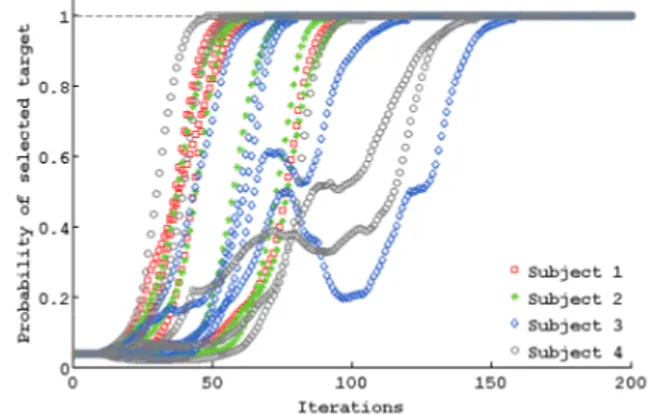
The algorithm was able to identify the correct target for all runs of all the subjects, see Figure 2. There are strong variations among subjects but we note that our system iden-tified each task in less iterations than a normal calibration phase requires (between 300 and 600 examples depend-ing on the user performance (Chavarriaga and Mill´an 2010; Iturrate, Montesano, and Minguez 2010)).
Figure 2: Results from the online experiment: Evolution of the probability of the correct task for each subject and run. The algorithm was able to identify the correct target for each subjects and runs in less than 200 iterations.
Table 1 shows for each subject and run the number of iterations needed to reach the confidence threshold for the subject selected target. On average, the number of iterations needed to identify the target was of 85± 32.
Run1 Run2 Run3 Run4 Run5 mean±std
S1 95 62 56 60 64 67 ± 16
S2 89 77 98 60 62 77 ± 17
S3 68 80 118 76 157 100 ± 37
S4 98 142 57 142 47 97 ± 45
Table 1: Results from the online experiment: Number of it-erations needed to identify the correct target for each sub-ject and run. On average, the number of iterations needed to identify the target was of 85± 32.
Algorithm Offline Analysis
The objective of the offline analysis is to study the impact of our exploration method and evaluate if the classifier learned from scratch with our algorithm can be reused for learning new tasks. Finally we want to evaluate how robust the sys-tem is to abrupt changes in the signal properties. For these experiments, to ensure we have sufficient data to achieve sta-tistically significant results, we rely on a large dataset of real EEG data. We used a dataset from (Iturrate, Montesano, and Minguez 2013b), which covers ten subjects that performed
two different control problems (denoted T1 and T 2). The role of the users was similar (assess the agent’s actions), but the problems differs in the state-action space size and visual representations. For each subject, T1 was composed of 1800 assessments, and T2 of 1200. Despite the fact that both problems elicit error-related potentials, the EEG sig-nals presented significant differences (Iturrate, Montesano, and Minguez 2013b).
For each subject, and each dataset (T1 and T 2), we sim-ulated20 runs of 400 iterations following the control task. Each time the device performed an action, we sampled the dataset using the ground truth labels corresponding to the correct task and then removed the chosen signal from it. Af-ter a first task was identified, and following our approach, we continued running the system to identify new tasks.
We present most of the results in terms of the quality of the dataset, measured as the classification accuracy that a calibrated brain signal classifier would obtain. Results vary strongly between subjects and we will see that it is a direct consequence of the difficulty of finding a classifier with high accuracy.
Planning Methods We compared the average number of steps (with maximum values of400 steps) needed to iden-tify the first task when learning from scratch with different planning methods. 0 50 100 150 200 250 300 350 400
Action selection methods
to identify first target
Number of iterations Uncertainty on signal ε−greedy ε=0.5 Random actions ε−greedy ε=0.1 Uncertainty on task Greedy
Figure 3: Comparison of different exploration methods. Our proposed method, based on the uncertainty on the task and the signals interpretation, allows to lead the system to re-gions that improve disambiguation among hypotheses in a faster way. For the greedy method, all values were400 which indicates it never allowed to identify any task.
Figure 3 shows the results averaged across subjects, runs and datasets. Values of400 means the confidence threshold was not reached after 400 iterations. Our proposed method, based on the uncertainty on the task and the signals inter-pretation, allows to lead the system to regions that improve disambiguation among hypotheses in a faster way. Trying to follow the most probable task does not allow the system to explore sufficiently (Greedy), and at least some random exploration is necessary to allow a correct identification of the task (ε-greedy). Assessing uncertainty only on the task performs poorly as it does not take into account the signal interpretation ambiguity inherent to our problem. The large variability in the results is mainly due to the large variations in classification accuracy across subjects and datasets. Given
these results, the remainder of this section will only consider our proposed planning method.
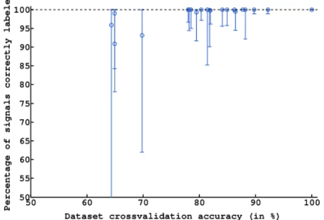
Online re-estimation of classifier After identifying the first task, and following our approach, we continued running the system and measured how many tasks were identified af-ter400 steps. The quality of our unsupervised method can be measured according to the percentage of labels correctly as-signed (according to the ground truth label), see Figure 4. In general, having dataset with classification accuracies higher than75% guaranteed that more than 90% of the labels were correctly assigned. This result shows that our algorithm can also be used to collect training data for calibrating any other state-of-the-art error-related potentials classifier, but has the important advantage of controlling the device at the same time. 50 60 70 80 90 100 50 55 60 65 70 75 80 85 90 95 100
Dataset crossvalidation accuracy (in %)
Percentage of signals correctly labeled
Figure 4: Percentage of labels correctly assigned according to the ground truth label (the markers show the median val-ues and the error bars the2.5th and 97.5th percentiles). In general, having dataset with classification accuracies higher than75% guaranteed that more than 90% of the labels were correctly assigned.
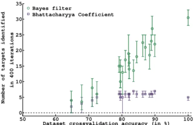
Figure 5 demonstrates the advantage of switching to a Bayes filter method after identification of a first target in-stead of keeping the estimation given by the Bhattacharyya coefficient. On the one hand, Bhattacharyya coefficient works very well for small amounts of data because it directly compares model parameters. On the other hand, when there is sufficient data, training a classifier allows for a faster iden-tification since the classifier makes a much harder decision when evaluating a new EEG signal.
Figure 6 shows the number of tasks correctly and incor-rectly identified in400 iterations. For datasets of good qual-ities, we are able to identify more than20 tasks in 400 it-erations without the need for a calibration procedure (re-cap that previous works needed between 300 and 600 exam-ples for the calibration phase (Chavarriaga and Mill´an 2010; Iturrate, Montesano, and Minguez 2010)). The number of correctly identified tasks is strongly correlated to the quality of the dataset.
50 60 70 80 90 100 0 5 10 15 20 25 30 35
Dataset crossvalidation accuracy (in %)
in 400 iterations
Number of targets identified
Bayes filter
Bhattacharyya Coefficient
Figure 5: Number of targets correctly identified in 400 it-erations (the markers show the median values and the er-ror bars the2.5th and 97.5th percentiles). Comparison be-tween switching to a Bayes filter method after identification of a first target instead of keeping the estimation given by the Bhattacharyya coefficient. The Bayes filter allows for a faster identification. 50 60 70 80 90 100 0 5 10 15 20 25 30 35
Dataset crossvalidation accuracy (in %)
in 400 iterations
Number of targets identified
True positive False positive
Figure 6: Number of targets correctly and incorrectly iden-tified in400 iterations (the markers show the median val-ues and the error bars the2.5th and 97.5th percentiles). For datasets of good qualities, we are able to identify more than 20 tasks in 400 iterations without the need for a calibration procedure.
Robustness to Abrupt Changes in the Signals’ Proper-ties We now want to determine whether the system is ro-bust to changes in the signals’ properties that occur when we change between different problem settings (Iturrate, Monte-sano, and Minguez 2013b). We modeled this by changing from T i to T j (i 6= j) after 400 steps, and then executing 400 more steps from T j. Both combinations (T 1 to T 2 and T2 to T 1) were tested.
Figure 7 shows the number of tasks identified depending on the classification accuracy on T j when training a classi-fier from dataset T i. For abrupt changes which conserve a classification accuracy above 70% on the new signals, our method, based on a limited size prior, is able to recover and solve more than 20 tasks in 400 iterations. For those cases where the accuracy change is too drastic, starting from
scratch may be a better solution than relying on the adapta-tion properties of our algorithm.
50 60 70 80 90 100 0 5 10 15 20 25 30 35
Dataset 1 to dataset 2 train/test accuracy (in %)
in 400 iterations
Number of targets identified
True positive False positive
Figure 7: Number of targets correctly and incorrectly iden-tified in400 iterations after an abrupt change in the signals properties (the markers show the median values and the er-ror bars the2.5th and 97.5th percentiles). For abrupt changes which conserve a classification accuracy above70% on the new signals, our method, based on a limited size prior, is able to recover and solve more than20 tasks in 400 iterations.
Conclusion
We introduced a novel method for calibration-free BCI based control of sequential tasks with feedback signals. The method provides an unsupervised way to train a decoder with almost the same performance as state-of-the-art super-vised classifiers, while keeping the system operational and solving the task requested by the user since the beginning. The intuition for our method is that the classification of the brain signals is easier when they are interpreted according to the task desired by the user. The method assumes a distri-bution of possible tasks and relies on finding which pair of decoder-task has the highest expected classification rate on the brain signals.
The algorithm was tested with real online experiments, showing that the users were able to guide an agent to a de-sired position by mentally assessing the agent’s actions and without any explicit calibration phase. Offline experiments show that we can identify an average of 20 tasks in 400 iter-ations without any calibration, while in previous works the calibration phase used between 300 and 600 examples. To improve the efficiency of the algorithm, we introduced a new planning method that uses the uncertainty in the decoder-task estimation. Finally, we analyzed the performance of the system in the presence of abrupt changes in the EEG signals. Our proposed method was able to adapt and reuse its learned models to the new signals. Furthermore, in those cases when the transfer is not possible, our method can still be used to recalibrate the system from scratch while solving the task.
A current limitation of the work is the need for a finite set of task hypotheses. This limitation could be solved by the use of a combination of particle filter and regularization on the task space. Additionally, our method can not dissoci-ate fully symmetric hypotheses, e.g. right and left most stdissoci-ate
of our 1D grid world (Fig. 1), as the interpretation of feed-back signals will also be symmetric and therefore as likely. This latter problem can be solved by redefining the set of hypotheses or the action set, for instance by adding a “stop” action valid only at the target state.
This work opens a new perspective regarding the global challenge of interacting with machines. It has application to many interaction problems which requires a machine to learn how to interpret unknown communicative signals. A promising avenue, outside the BCI field, lies in human robot interaction scenarios where robots must learn from, and in-teract with, many different users who have their own limita-tions and preferences.
Acknowledgments
The authors would like to thank the anonymous reviewers for their helpful comments which contributed in improv-ing the quality of this paper. The authors from INRIA are with the Flowers Team, a join INRIA - Ensta ParisTech lab, France. Luis Montesano is with Instituto de Investi-gaci´on en Ingenier´ıa de Sistemas, Universidad de Zaragoza, Spain. I˜naki Iturrate is with the Chair in Non-invasive Brain-Machine Interface (CNBI) and Center for Neuroprosthet-ics and Institute of Bioengineering, EPFL, Switzerland. This work has been partially supported by INRIA, Con-seil R´egional d’Aquitaine and the ERC grant EXPLORERS 24007; and from the Spanish Ministry via DPI2011-25892 (L.M.), and DGA-FSE grupo T04.
References
Bengio, Y., and Grandvalet, Y. 2004. No unbiased estima-tor of the variance of k-fold cross-validation. The Journal of
Machine Learning Research5:1089–1105.
Blankertz, B.; Lemm, S.; Treder, M.; S., H.; and M¨uller, K.-R. 2010. Single-trial analysis and classification of ERP compo-nents: A tutorial. Neuroimage.
Brafman, R., and Tennenholtz, M. 2003. R-max a general polynomial time algorithm for near-optimal reinforcement learning. Journal of Machine Learning Research 3.
Chavarriaga, R., and Mill´an, J. 2010. Learning from EEG error-related potentials in noninvasive brain-computer inter-faces. Neural Systems and Rehabilitation Engineering, IEEE
Transactions on18(4):381–388.
Falkenstein, M.; Hoormann, J.; Christ, S.; and Hohnsbein, J. 2000. ERP components on reaction errors and their functional significance: A tutorial. Biological Psychology 51:87–107. Ferrez, P., and Mill´an, J. 2008. Error-related EEG poten-tials generated during simulated Brain-Computer interaction.
IEEE Trans Biomed Eng55(3):923–929.
Friedman, J. H. 1989. Regularized discriminant analysis.
Journal of the American statistical association84(405):165–
175.
Grizou, J.; Lopes, M.; and Oudeyer, P.-Y. 2013. Robot learn-ing simultaneously a task and how to interpret human in-structions. In Joint IEEE International Conference on
De-velopment and Learning and on Epigenetic Robotics
(ICDL-EpiRob).
Iturrate, I.; Montesano, L.; and Minguez, J. 2010. Single trial recognition of error-related potentials during observation of robot operation. In Engineering in Medicine and Biology
Society (EMBC), 2010 Annual International Conference of
the IEEE, 4181–4184. IEEE.
Iturrate, I.; Montesano, L.; and Minguez, J. 2013a. Shared-control brain-computer interface for a two dimensional
reach-ing task usreach-ing EEG error-related potentials. In Int. Conf.
of the IEEE Engineering in Medicine and Biology Society
(EMBC). IEEE.
Iturrate, I.; Montesano, L.; and Minguez, J. 2013b. Task-dependent signal variations in EEG error-related potentials for brain-computer interfaces. Journal of Neural Engineering 10(2).
Kailath, T. 1967. The divergence and Bhattacharyya distance measures in signal selection. IEEE Trans. Commun. Technol. 15(3):52–60.
Kindermans, P.-J.; Verschore, H.; Verstraeten, D.; and Schrauwen, B. 2012. A P300 BCI for the Masses: Prior Information Enables Instant Unsupervised Spelling. In NIPS, 719–727.
Kindermans, P.-J.; Verstraeten, D.; and Schrauwen, B. 2012. A bayesian model for exploiting application constraints to en-able unsupervised training of a P300-based BCI. PloS one 7(4):e33758.
Kolter, J. Z., and Ng, A. Y. 2009. Near-Bayesian exploration in polynomial time. In International Conference on Machine
Learning. ACM.
Ledoit, O., and Wolf, M. 2004. A well-conditioned estimator for large-dimensional covariance matrices. Journal of
multi-variate analysis88(2):365–411.
Lee, C., and Choi, E. 2000. Bayes error evaluation of the Gaussian ML classifier. Geoscience and Remote Sensing,
IEEE Transactions on38(3):1471–1475.
Mill´an, J.; Rupp, R.; M¨uller-Putz, G. R.; Murray-Smith, R.; Giugliemma, C.; Tangermann, M.; Vidaurre, C.; Cincotti,
F.; K¨ubler, A.; Leeb, R.; et al. 2010. Combining
brain-computer interfaces and assistive technologies: state-of-the-art and challenges. Frontiers in neuroscience 4.
Orsborn, A.; Dangi, S.; Moorman, H. G.; and Carmena,
J. M. 2012. Closed-Loop Decoder Adaptation on
In-termediate Time-Scales Facilitates Rapid BMI Performance Improvements Independent of Decoder Initialization Condi-tions. IEEE Trans. on neural systems and rehabilitation
en-gineering20(4).
Polich, J. 1997. On the relationship between EEG and P300: individual differences, aging, and ultradian rhythms.
Interna-tional Journal of Psychophysiology26(1-3).
Sutton, R., and Barto, A. 1998. Reinforcement learning: An
introduction. MIT press.
Tangermann, M.; Kindermans, P.-J.; Schreuder, M.;
Schrauwen, B.; and M¨uller, K.-R. 2013. Zero training
for BCI-reality for BCI systems based on event-related potentials. Biomed Tech 58:1.
Vidaurre, C., and Blankertz, B. 2010. Towards a cure for BCI illiteracy. Brain topography 23(2):194–198.
Vidaurre, C.; Kawanabe, M.; von Bunau, P.; Blankertz, B.; and M¨uller, K.-R. 2011. Toward unsupervised adaptation of LDA for brain-computer interfaces. Biomedical Engineering,