Estimating fat, paste and gas in a proving Danish paste by MRI – Description of the method and evaluation of its performances (bias and accuracy, sensitivity threshold)

HAL Id: hal-00835832

https://hal.archives-ouvertes.fr/hal-00835832v5

HAL is a multi-disciplinary open access archive for the deposit and dissemination of sci-entific research documents, whether they are pub-lished or not. The documents may come from teaching and research institutions in France or abroad, or from public or private research centers.

L’archive ouverte pluridisciplinaire HAL, est destinée au dépôt et à la diffusion de documents scientifiques de niveau recherche, publiés ou non, émanant des établissements d’enseignement et de recherche français ou étrangers, des laboratoires publics ou privés.

Estimating fat, paste and gas in a proving Danish paste

by MRI – Description of the method and evaluation of

its performances (bias and accuracy, sensitivity

threshold)

Guylaine Collewet, Vincent Perrouin, Cécile Deligny, Jérôme Idier, Tiphaine

Lucas

To cite this version:

Guylaine Collewet, Vincent Perrouin, Cécile Deligny, Jérôme Idier, Tiphaine Lucas. Estimating fat, paste and gas in a proving Danish paste by MRI – Description of the method and evaluation of its performances (bias and accuracy, sensitivity threshold). 2016. �hal-00835832v5�

Estimating fat, paste and gas in a proving Danish paste by MRI –

Description of the method and evaluation of its performances (bias and

accuracy, sensitivity threshold)

Guylaine Collewet1, Vincent Perrouin1,Cécile Deligny1, Jérôme Idier2, Tiphaine Lucas1

1 : IRSTEA, UR OPAALE, 17 avenue de cucillé, CS 64427, 35044 Rennes, France 2 : IRCCyN CNRS, F-44300 Nantes, France

1 Introduction

The aim of the method presented in this paper is to characterize the development of the structures of Danish pastes during proving. Danish pastes are made of layers of fat and dough, which is itself composed of paste (gas-free dough) and gas. During the proving, the dough is expanding, its gas fraction is increasing and gas bubbles are developing. It is interesting to observe the evolution of the expansion which can be characterized in different ways. First of all, it is important to detect the layers of fat since they play a significant role in the development of the pastry. For example, it is interesting to determine whether they are continuous or not. It is also interesting to measure the evolution of the gas fraction of the different layers of dough, delimitated by the layers of fat, to detect the potential formation of large bubbles and to observe if they develop in specific areas such as near or far from the layers of fat.

Most reports on puff and Danish pastries are fairly old, dating from the 70’s-90’s. Their approach was mostly technology-orientated and observations were global and focused on the dimensions of the product. Indeed, like many bakery products, the alveolar structure of puff and Danish pastries is fragile and may collapse if intrusive measurement techniques are used during processing. Pictures of baked alveolar structures were more rarely reported, and still lacked quantitative analysis (Deligny & Lucas, 2015) (Filloux, 2008) (Cauvain & Telloke, 1993). Recent advances in the techniques of imaging and image analysis offer new opportunities for capturing the structural elements in bakery products together with their changes during processing. This opens up the possibility to re-explore the mechanisms governing expansion in these kinds of product. In this study we focused on proving.

Among the recently developed techniques, Magnetic Resonance Imaging (MRI), widely used for medical diagnosis, can be used for food applications to determine the state of water, composition and/or structure of macromolecules in foodstuffs. Indeed, the MRI signal is sensitive to both the density and the mobility of the protons. MRI also provides a good trade-off between spatial and time resolution which makes possible the dynamic monitoring of a process step (mass transfer, baking, freezing, and thawing). To date, MRI has not been applied to Danish pastry. Likewise, there is a broad literature about MRI applied to (bread) dough or fat when considered separately. The major advances and limits in these two applications are presented below. These are highlighted by comparison with X-rays tomography, which may constitute an alternative to MRI in some cases.

The proportion and morphology of the gaseous phase in bread dough has been extensively studied by MRI. MRI voxels filled only with gas, and thus presenting a nil or low signal intensity, were analyzed in the early studies (Van Duynhoven et al., 2003) (Takano, Ishida, Koizumi, & H.Kano, 2002). Given this objective, the images were acquired using so-called “spin echo sequences” since it is a protocol known to minimize artifacts of magnetic susceptibility between gas and water fractions, that are responsible for local deformation. Large-sized bubbles (> 1 mm2) only were visible and served for further quantitative analysis (Van Duynhoven, et al., 2003). Higher spatial resolution with MRI (Goetz, Gross, & Koehler, 2003) (Bonny et al., 2004) (Rouille, Bonny, Della Valle, Devaux, & Renou, 2005) (Bajd & Sersa, 2011) were attained in later studies to the price of higher acquisition times (7-30 min versus 2-4 min in earlier studies), inducing

movement blurring because of dough inflation, and altering quantification; high spatial resolution is also compatible with small-sized samples only (1-3 cm in the above mentioned studies) and does not permit studying real sized products. X-ray tomography is another noninvasive technique with which it is possible to monitor the changes in density during bread dough proving (Babin et al., 2006; Bellido, Scanlon, Page, & Hallgrimsson, 2006; Turbin-Orger et al., 2012; Whitworth & Alava, 1999). Short acquisition times (a few seconds) can be achieved with this technique. However limits in the spatial resolution are roughly the same as for MRI and the so-called “partial volume effect” (voxels containing more than one component, gas and paste in the case of bread) is largely encountered with both techniques. When partial volume was analyzed, the proportionality between the signal measured and the gas fraction was always assumed. In the case of partial volume with MRI, the potential effects of variations in temperature or composition (upon yeast activity for instance) on the signal of paste during proving were ignored (Grenier, Lucas, Collewet, & Le Bail, 2003; Grenier, Lucas, Davenel, Collewet, & Le Bail, 2003) (Lucas, Grenier, Bornert, Challois, & Quellec, 2010).

As regards to the quantification of fat, X-ray tomography provides the contrast needed. Indeed the density of fat is different from other tissues in living organisms and thus pure fat deposits can easily be segmented from muscle and bone, as for example in pig carcasses (Furnols, Teran, & Gispert, 2009) and in fish (Kolstad, Vegusdal, Baeverfjord, & Einen, 2004). However, in the case of voxels containing a mixture of paste, fat and gas as in puff and Danish pastries, it would not be possible to quantify all the components within. Indeed X-ray provides only one image and only the sum of the contribution of all the material within a voxel can be measured (Artz et al., 2012). In the case of more than two components contributing to the signal intensity in a given voxel, one image is not sufficient to unravel the contributions of each component. More flexible, MRI imaging can provide the information needed to measure the proportion of several components within a voxel. It has for example been successfully used for intra-voxel fat quantification in fish (Collewet et al., 2013).

In the case of this application, the use of MRI faces two problems, which are the relative small spatial resolution and the low value of the signal to noise ratio (𝑆𝑁𝑅) particularly at the end of the proving when the dough contains much gas that gives no signal. The signal is thus decreasing in the dough during proving. The 𝑆𝑁𝑅 and the spatial resolution are linked by the following relations:

𝑆𝑁𝑅 ∝ ∆𝑉√𝑡𝑎𝑐𝑞 ₍₁₎

∆𝑉 = 𝐿𝑥𝐿𝑦

𝑁_𝑥𝑁_𝑦 𝑒 (2)

𝑡_𝑎𝑐𝑞= 𝑇𝑅 𝑁_𝑦𝑁_𝑎𝑐𝑐 (3)

where ∆𝑉 is the elementary volume which corresponds to one voxel1 _{of the image, 𝐿}

𝑥 and 𝐿𝑦 are the size of the field-of-view in both directions of the image-plane, 𝑒 is the thickness of the virtual slice, 𝑁_𝑥 and 𝑁_𝑦 are the number of the voxels in the image (number of lines and columns). 𝑡_𝑎𝑐𝑞 is the acquisition time, 𝑁_𝑎𝑐𝑐 is the number of the repetitions of the acquisitions before averaging the signal, in order to reduce the noise and 𝑇𝑅 is the so-called repetition time which also influences the contrast in the images.

Thus, the values of 𝑆𝑁𝑅, ∆𝑉 and 𝑡_𝑎𝑐𝑞 are linked and the choice of the acquisition parameters is a compromise between getting a high 𝑆𝑁𝑅, a high spatial resolution (ie a small ∆𝑉) and a short 𝑡_𝑎𝑐𝑞. One way to increase the 𝑆𝑁𝑅 would be to increase the acquisition time. However, as we want to follow the expansion of the dough, the acquisition time should be limited in order to avoid movement artefacts in the images. Concerning the value of ∆𝑉 it would be interesting to set it such that the thin layers of fat would be represented by a line thick of a few pixels in the images. However, a too small value of ∆𝑉 would imply a low value for 𝑆𝑁𝑅. Finally, along with the intrinsic limitations of MRI, these constraints will set the values of ∆𝑉 on the order of 1mm3

. Since the thickness of the layers of fat are in the order of 0.1 mm, this leads to

1 _{In MRI one picture element, or pixel, of the image is called a voxel since the signal is the sum of the signals of all the}

partial volume effects, that is, each voxel of the image will contain a mixture of fat and dough. The same phenomenon will be observed with dough and gas, since the size of the smallest bubbles does not exceed the resolution of the image. Thus, the MRI images for this application will present relatively low 𝑆𝑁𝑅 combined with a strong partial volume effect. As this will be detailed in the paper, this led us to develop a method able to estimate in each voxel the quantity of each component, fat, paste and gas while adding some spatial regularization in order to reduce the effects of the noise.

This report is organized as follows: firstly we will present the model of the MRI signal. As each voxel corresponds to a mixture of components, the signal will be modelled as the sum of the signal of each component. This will lead to the estimation of several unknowns for each voxel which are the proportions of each component. This implies the use of several images acquired with different acquisition parameters and also the knowledge of “reference signals” for each component. The estimation of the unknowns comes down to find the solutions of a criterion composed of the squared difference between the data and the model. In order to get rid of the unwanted effects of the noise, this criterion is completed with a regularization term imposing solutions with a relative spatial smoothness. The optimization algorithm used to minimize this criterion is detailed. Then several simulation results are presented. First of all the choice of realistic numerical values corresponding to the targeted application is presented. Then the setting of the parameters of the algorithm is detailed. Finally, the results are divided in two parts. First of all we ran simulations in order to assess the theorical performance of the method: we explored the case where reference signals are perfectly known and we also studied the influence of the uncertainty on these reference signals using Monte-Carlo simulations. Then we validated the method on genuine MRI images of Danish paste, by checking the conservation of the total proportion of fat and paste.

2 Measurement method

2.1 Signal model

The model of the MRI signal depends on the acquisition protocol. Indeed, this imaging modality offers different ways to acquire a signal. In our case of interest, two kinds of protocol could be considered. The first one is the “spin echo” protocol (SE) which provides a complex signal (with a real and imaginary value) the phase (also called argument) of which is the same whatever the components. Thus, in this case, there is no loss of signal when adding the signals of the different components. The amplitude depends on the characteristics of the component which allows distinguishing between fat and paste. The second one is the “gradient echo” protocol (GE) which is routinely used to quantify fat. Indeed, this protocol provides a signal the phase of which is different for fat. This property can be used also to quantify fat. However, this protocol is prone to be sensitive to local magnetic field variations, which typically occur at the interfaces with gas. This leads to unexpected loss of the signal, especially in the dough where many small bubbles of gas are present. This would give images with no signal for the dough. For this reason we chose to use the SE protocol.

As explained in the introduction, we considered that each voxel contains a mixture of an unknown proportion of three components, fat, paste and gas. We made the hypothesis that the signal of each component did not vary with the localisation within the pastry, in other words that the signal of a voxel filled with fat or paste would not depend on the position in the pastry. When the sample is large regarding the size of the coil which acquires the signal, unwanted variations of the signal can be observed near the border. We assumed that, thanks to the small size of the sample and to its positioning in the centre of the coil, the signal could be considered as independent of the position. Thus, under these hypothesis, the signal 𝑠_𝑥𝑘𝑡∗ , for each voxel 𝑥, in absence of noise, at time 𝑡, with the set of acquisition parameters 𝑘 can be modelized by:

𝑠_𝑥𝑘𝑡∗ _{= ∑ 𝑂} 𝑖𝑘𝑡𝑝𝑥𝑖𝑡 𝐼 𝑖=1 (4) subject to ∑ 𝑝𝑥𝑖𝑡= 1 𝐼 𝑖=1 (5)

where 𝐼 is the number of components, which will be set to 3 in the present study, 𝑝_𝑥𝑖𝑡∈ [0 ,1] stands for the proportion of component 𝑖 in voxel 𝑥 at time 𝑡, 𝑂𝑖𝑘𝑡, referred hereafter as “reference signals”, corresponds to the signal of a voxel filled with component 𝑖 at time 𝑡, with the set of parameters 𝑘. In the remainder of the paper 𝑖 will be equal to 𝑓, 𝑝 and 𝑔 respectively for fat, paste and gas.

It is to be noted that the reference signals are subject to vary with time mainly because of the variation of the temperature; this point will be further discussed in section 2.4.

In MRI, the signal of an image acquired with the parameters 𝑘 corresponds to the modulus of a complex number, the real and imaginary parts of which are added with a centered gaussian noise with the same variance 𝜎_𝑘2_{. Thus the noise corruption of the MRI signal is not gaussian but follows a rician law. Taking this} into account, under the non-reductive hypothesis of a phase equal to 0, leads to model the rician-noised signal 𝑠_𝑥𝑘𝑡𝑅 _{, where 𝑅 stands for rician, as :}

𝑠_𝑥𝑘𝑡𝑅 _{= √(𝑠}

𝑥𝑘𝑡∗ + 𝑛𝑥𝑘𝑟)2+ 𝑛𝑥𝑘𝑗2 ₍₆₎

where 𝑛_𝑥𝑘𝑟 and 𝑛_𝑥𝑘𝑗 are respectively the gaussian additive noise on the real and on the imaginary parts of the complex signal for voxel 𝑥. For the sake of simplification, we will consider hereafter that the noise is not rician but gaussian and additive with a variance equal to 𝜎_𝑘2. It can be shown that this hypothesis stands for 𝑆𝑁𝑅 > 3 (Gudbjartsson & Patz, 1995). However, as it will been shown later, 𝑆𝑁𝑅 can be lower than 3 in images of proving Danish pastry which will lead to some bias of the results. The model 𝑠_𝑥𝑘𝑡 of the signal we used was the noise-free signal added with gaussian noise and expressed as :

𝑠_𝑥𝑘𝑡= 𝑠_𝑥𝑘𝑡∗ _{+ 𝑛}

𝑥𝑘, ₍₇₎

where 𝑛_𝑥𝑘 is a gaussian centered noise with variance 𝜎_𝑘2_.

The model of the signal being expressed, we are going to detail how we will estimate the unknowns.

2.2 Estimation of the unknowns

First of all, we considered that 𝑂_𝑖𝑘𝑡 can be measured separately and once for all using homogeneous block of fat and of paste. This point will be detailed later. Moreover, 𝑂_𝑖𝑘𝑡 will be set to 0 for gas, whatever the temperature, since this component gives no signal. Thus, the unknowns are 𝑝_𝑥𝑖𝑡 which amounts, at one time 𝑡, to 𝐼 images, i.e. 𝐼𝑋 scalar unkowns noting 𝑋 the number of voxels in the image. Given constraint (5) this amount drops to (𝐼 − 1) scalar unknowns per voxel, and thus (𝐼 − 1)𝑋 scalar unknowns in total. For the remainder of the paper, in order to lighten the notations, we will note the unknowns 𝑝𝑥𝑖. This is possible since, as it will be explained later, the estimation will be realised separately for each time 𝑡. 𝑝𝑥𝑖 thus refer to the unknowns in the current image.

In order to build reliable estimates, we propose to acquire 𝐾 ≥ 𝐼 − 1 images using different values of parameters 𝑘. This is possible in MRI since different settings of the protocol parameters lead to different signal amplitudes. This will lead to different values of 𝑂_𝑖𝑘𝑡.

Moreover, in a view to reduce the noise, some regularization on the component proportions 𝑝_𝑥𝑖 can also be introduced. However, it should be carefully designed, so that large variations of the signal be not penalized at the boundaries between distinct regions of the object namely the layers of fat and dough or large bubbles inside dough. In this paper, we adopt an approach so-called edge-preserving in the field of image restoration. More precisely we propose to estimate 𝒑 = (𝑝_𝑥𝑖) using a penalized least-square approach:

𝒑̂ = arg min 𝒑 𝒥(𝒑) (8) where 𝒥(𝒑) = ∑ 𝜆_𝑘∑ (𝑠_𝑥𝑘𝑡− ∑ 𝑂_𝑖𝑘𝑡𝑝_𝑥𝑖 𝐼 𝑖=1 ) 2 + 𝛾 ∑ Φ(‖𝒅_𝑐𝑡_𝒑‖) 𝑐𝜖𝒞 𝑋 𝑥=1 𝐾 𝑘=1 (9)

Since Φ is strictly convex, it can be easily shown that 𝒥 is strictly convex w.r.t. 𝒑, and, therefore, a unimodal function of 𝒑. However, The minimization of 𝒥 is not trivial since 𝒥 is not a quadratic function of 𝒑. We used a non-linear conjugate gradient (CG) algorithm such as the one detailed in (Labat & Idier, 2008) to minimize 𝒥 w.r.t 𝒑, subject to constraint (2). CG algorithm is iterative. We initialized the solution with the one that minimizes the first term in (9) which corresponds to a least-squares minimization. This is easily computable since it is separable (the solution for each voxel is independent from the others) . Then we iterated the CG steps until the norm of the gradient of 𝒥 w.r.t 𝒑 becomes sufficiently small, i.e. ‖∇𝒥(𝒑)‖ ≤ 𝜀.

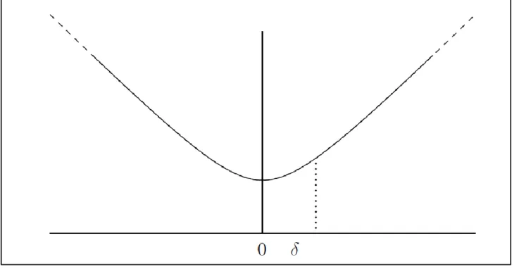
One key point of our method is the choice of the hyperparameters 𝜆_𝑘, 𝛾 and 𝛿. According to the probabilistic interpretation of criterion, 𝜆_𝑘 corresponds to the inverse of the noise variance for the kth image. The noise variance can be estimated directly from the images using the method proposed in (Nowak, 1999). Two parameters remain to be adjusted. Their settings are made using simulations results as this will be developed later on. As these simulations require some realistic numerical values for all the variables, we first detail how we determined them.

2.3 Choice of the parameters k and MRI protocol

In the case of SE protocol the reference signals can be written as:

𝑂𝑖𝑘𝑡 = 𝐺𝜌𝑖𝑡𝑒−𝑇𝐸𝑘⁄𝑇2𝑖𝑡(1 − 𝑒−𝑇𝑅𝑘⁄𝑇1𝑖𝑡), (10)

where G represents the global gain of the acquisition system, 𝜌𝑖𝑡, 𝑇2𝑖𝑡 and 𝑇1𝑖𝑡 respectively the proton density, transversal and longitudinal relaxations times for component 𝑖 at time 𝑡. 𝑇𝐸𝑘 is the so-called “echo time” and is a parameter chosen by the user, as well as the values of the repetition time 𝑇𝑅_𝑘. Preliminary measurements on a block of fat and a block of dough with a fixed proportion of gas (dough was prepared by mixing ingredients to the exclusion of yeast) showed that there was not much difference between the 𝑇₁ of

susceptible to make the relaxation times vary. 𝑇₁ varied from 190 ms for paste and 175 ms for fat at 15°C, i.e. at the beginning of the proving, to 236 ms for paste and 230 ms for fat at 30°C, i.e. at the end of the proving. On the contrary the values of 𝑇2 were different: 𝑇2 was around 23 ms for paste whatever the temperature and varied from 37 ms at 15°C to 82 ms at 30°C for fat. This led naturally to the choice of 𝑇2 -weighted contrast images, that is images with different values of 𝑇𝐸_𝑘. It is to be noted that this can be done without increasing the acquisition time since the acquisition of at least 2 images can be achieved using so-called “multi spin echo sequences”. Regarding the constraints of our MRI system, the only sequence available was a SE sequence with maximum two echoes.

In order to choose the best 𝑇𝐸𝑘 we computed the Cramer-Rao bound (Rao, 2008) for the first term of equation (4), that is we ignored the regularisation term at this stage. We chose to determine the best 𝑇𝐸_𝑘 for the temperature at the end of the proving (30°C). Measurements on a block of fat and a block of paste were realized at this temperature using a spin echo sequence with different 𝑇𝐸. The MRI protocol described in this section was used. These acquisitions, as well as all the subsequent ones, were realised with a 1.5T Avanto MRI system (Siemens) equipped with a “knee coil”. This led to the estimation of 𝑇_2𝑡 and 𝑀0𝑡 = 𝐺𝜌_𝑡(1 − 𝑒−𝑇𝑅 𝑇⁄1𝑡) for the fat and for the paste. Thanks to these values we computed Cramer-Rao bounds

for different combinations of 𝑇𝐸₁ and 𝑇𝐸₂. The lower Cramer-Rao bound for the estimation of fat and paste was for 𝑇𝐸₁ = 7 ms and 𝑇𝐸₂ = 32 ms.

The other acquisition parameters were set as follows: we set the field of view to 40 x 160 mm2 which is a bit larger than the maximum size of the Danish paste at the end of the proving. The resolution was set to 0.5 x 0.5 mm2 with a slice thickness of 3 mm. This led to a number of lines 𝑁_𝑦= 40 0.5 =⁄ 80. The other parameters were set so as to get acceptable 𝑆𝑁𝑅 and acquisition time. The rate of dough expansion was evaluated by MRI in order to determine the maximum acquisition time. It appeared that when the expansion is the fastest and presents a linear behaviour with time, the height of a Danish pastry with 4 layers of fat increased by 10 mm per hour. We decided that the increase in height during an acquisition should be less than 1 mm and the maximum acquisition duration was set to 5 minutes. Regarding theses constraints 𝑇𝑅𝑘 was set to 400 ms for 𝑘 = 1 and 2 so as to get a relatively high level of the signal regarding equation (10). The number of accumulations 𝑁𝑎𝑐𝑐 was 9 so as to lead to an acquisition time 𝑡𝑎𝑐𝑞= 4mn 48 sec. The bandwidth acquisition was set to 230 Hz/pixel. Moreover, without increasing the acquisition time it was possible to acquire several slices in order to cover the whole product (typically 6 or 8 depending on the size). We also acquired images with these parameters in order to measure the level of the noise in these conditions. The variance of the noise was estimated using the method proposed in (Nowak, 1999). We measured a variance equal to 12.25.

2.4 Measurement of the reference signals

This part of the study aimed at measuring 𝑂_𝑖𝑘𝑡 as set out in Equation (4). Samples of pure component 𝑖 were placed in the MRI probe within the same area as that used for the Danish paste during proving. The MRI protocol described in section 2.3 was used.

2.4.1 Fat reference signal

𝑶

For the fat component, time course changes of the reference signals are due to temperature, increasing from 17°C (room temperature for lamination) to 30°C (proving temperature). Hence, for the measurement of 𝑂_𝑓𝑘𝑡, the temperature of fat samples was gradually increased in the range of 20 to 40°C. A period of 90 min was applied after each change in temperature setting to reach the new thermal equilibrium. For these measurements and all the subsequent ones, temperature was measured with pre-calibrated optical fibers (type T, 1 mm thick) inserted within the Danish paste, and recorded every 10 s during proving using a data acquisition Luxtron 790 connected to a PC. Fig 2 shows the reference signals of fat for the two TE values, 𝑂_𝑓1𝑡 and 𝑂_𝑓2𝑡, as a function of the temperature. The increase of the MRI signal of fat with the increase in

temperature (by a factor of 1.5-4) was mainly due to the melting of fat crystals. We approximated the evolution with temperature with a polynomial function in the order of 2. For the application of the mapping method, the temperature 𝜃_𝑡 at core of the Danish paste was hence monitored simultaneously to MRI during proving. Knowing 𝜃_𝑡, the reference signal of fat as a function of time, 𝑂_𝑓𝑘𝑡 , was deduced from the equations given in Fig 2.

2.4.2 Gas-free dough reference signal

𝑶

Time-course changes in temperature, in composition due to yeast activity (leading to the production of smaller sugars and of CO2 with action on the pH), and in hydration (e.g. starch granules, remaining

crystallites of salt) of the components constituting the gluten-starch matrix of the dough may affect the reference signal of the paste during proving. Separating the time-course changes in the signal of paste during proving from those due to the increasing proportion of gas was the complex part of this task, because it is difficult to prepare a dough without incorporating gas.

For this purpose, the signal of base dough alone (without fat) was monitored by MRI from the very end of the mixing step. Base dough was not laminated but sampled just after mixing and was gently sheeted down to 7 mm thick to avoid degasing. A rectangle (10 cm×5 cm) was cut from the center of the dough sheet and placed in a plastic container for proving. It was placed immediately inside the MRI probe and continuously monitored since then. Since the yeast activity is temperature- and time- dependent, the same thermal history as that of Danish paste (Fig 3) was applied to the base dough with the aid of a temperature-controlled device placed inside the MRI probe (Lucas et al., 2010). For this purpose, each step of the paste processing was characterised by duration together with an average temperature or a constant rate of heating/cooling. The total duration associated to the lamination step was relevant of three sheeting steps (17 min each, at an average temperature of 16°C), and thus applicable to the preparation of a 8 or 12 fat layers Danish paste. The mean signal of base dough, 𝑆̅_𝑑𝑘𝑡, for parameter k at time t of the proving process is written:

𝑆̅_𝑑𝑘𝑡 = 𝑂_𝑝𝑘𝑡(1 − 𝑝̅_𝑔𝑡) (11)

where 𝑝̅𝑔𝑡 is the mean proportion of gas, i.e. the mean volume of gas in relation to the base dough volume at time t. Thus, in order to estimate the reference signal of the gas-free dough 𝑂𝑑𝑘𝑡 from 𝑆̅𝑑𝑘𝑡, we needed to know 𝑝̅_𝑔𝑡. For this purpose, we used the following equation between the total volume of the base dough and the mean proportion of gas (Grenier et al., 2003):

𝑝̅_{𝑔 𝑡} = 1 −𝑉𝑟𝑒𝑓

𝑉_𝑡 (1 − 𝑝̅𝑔 𝑟𝑒𝑓)

(12) where 𝑉_𝑡 = 𝑛_𝑡∆𝑉 is the volume of the base dough at time 𝑡 (with 𝑛_𝑡 the number of voxels and ∆V the volume of a voxel) assuming that proving takes place mainly in this plane of observation. To verify this hypothesis, the sample was placed in a plastic container, the internal dimensions of which closely fitted the external dimensions of the dough sample in width and length. The dough sample was thus allowed to expand mainly in the upward direction. In order to evaluate 𝑛𝑡 the set of voxels belonging to the product was separated from the background using an algorithm applied on the MRI image acquired at TE=7 ms. It was based on the “active contours” (Chan & Vese, 2001). It detected the region presenting the highest intensity gradient in the image. Once the contour was detected, the inner part (section of the product) was easily determined as well as its volume 𝑉𝑡 directly linked to 𝑛𝑡. Considering that the expansion was symmetric, the measurement of 𝑉_𝑡was realised in the central slice. 𝑝̅_{𝑔 𝑟𝑒𝑓} can be considered to be 10% at the end of mixing, which is an average value for different types of kneaders, working at different speeds e.g. (Cauvain, Whitworth, & Alava, 1999)).

𝑝̅_{𝑔 𝑡} can then be estimated from Equation (12) at any processing time, starting MRI monitoring from the end of mixing.

𝑂_𝑝1𝑡 is presented in Fig 3 from the end of mixing to the end of proving. Since temperature little affected the NMR relaxation of dough (section 2.3), these observed changes during the paste preparation and proving were assigned to hydration (of proteins mainly) and yeast activity respectively. As the total amplitude of variation for 𝑂𝑝1𝑡 was of about 15 a.u. during proving (0<t<180 min), 𝑂𝑝1𝑡 was set at 325 a.u. in the mapping method. Similar observations were made for 𝑂𝑝2𝑡, the value of which was set at 60 a.u.

2.4.3 Spatial uniformity of the reference signals

The reference signals were supposed not to depend on the position in the Danish paste, as well as the position of the Danish paste. The validity of this assumption is discussed below to the light of complementary, yet preliminary measurements.

On the one hand, average values only were presented in sections 2.4.1 and 2.4.2. Dispersion around the average was due to noise, but also to spatial variations in the material used for calibration. Among all tested sources of spatial variation (including the composition of the reference material), that produced by the inhomogeneities of the coil, used to acquire the signal, was the highest. On images of a homogeneous object (a bottle filled of water, at stabilized temperature), a spatial variation in the MRI signal was observed. Its amplitude was of up to 15% inside the volume occupied by the 4 central slices over the 8 acquired. Nevertheless it was chosen not to model these spatial variations in a first approximation.

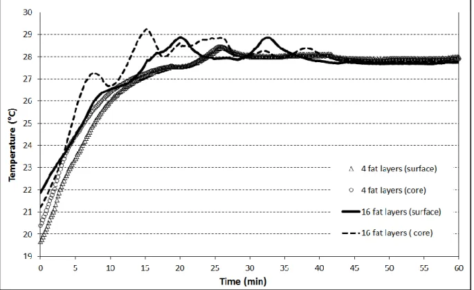
On the other hand, the reference signal of fat is calculated with the aid of core temperature in Danish paste. A gradient in temperature could develop because of heat transport through the thickness of the paste. Biot number, which represents the ratio between thermal resistances outside and inside the Danish paste, was lower than 1, suggesting the status of a thin thermal body (small gradient in temperature). This was confirmed by temperature measurements at the surface and in the core of Danish paste samples (difference not exceeding 1°C, in Figure 4). This second source of spatial variation was also neglected in a first approximation.

2.5 Setting of the values of

𝜸 and 𝜹

Once the protocol defined and the reference signals determined with this protocol, it is possible to set the parameters 𝛾 and 𝛿 which drive the regularisation properties of the estimation algorithm. These parameters were set using simulations on virtual Danish pastes, as detailed below.

We ran successive simulations with 𝛾 varying from 500 to 10000 by steps of 500 and 𝛿 varying from 0.05 to 0.6 by steps of 0.05. The set of values for 𝛾 was chosen empirically since no probable value can be inferred a

priori. On the contrary, the value for 𝛿 can be compared with the value of ‖𝒅𝑐𝑡𝒑‖ which corresponds to the difference between the component proportion of one given voxel and of the voxel of the corresponding neighbourhood 𝒞. Indeed 𝛿 can be considered as a threshold above which the Φ function is no more quadratic. As 𝑝_𝑥𝑖 represents component proportion ∈ [0 ,1], we chose values from 0.05 to 0.6.

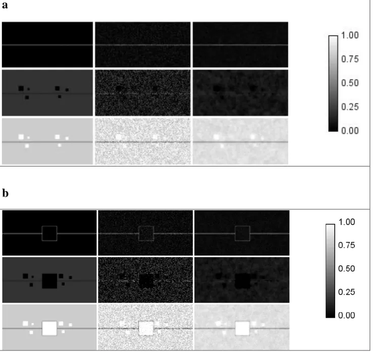
The simulations were carried out on virtual Danish pastes, simplified to a basic structural element composed of a unique layer of fat surrounded by an homogeneous dough. The thickness of the fat layer was set to 200, 100 or 50 m which corresponds to an ideal four, eight and sixteen layers pastry for an initial thickness of fat representing one third of the total thickness of the primary book and a Danish paste sheet rolled out down to 4 mm. These three cases will be referred as to four-fat layers, eight-fat layers and sixteen-fat layers although the virtual images contained a single fat layer only. The reference signals of fat were computed considering either 22°C at the beginning of the proving or 30°C at the end. Likewise, the gas proportion in dough was set at either 20% or 80% in order to cover the range of variations during proving (see Figure 5, especially maps of gas proportions); in the latter case, some bubbles full of gas, of different sizes were also added: 3.5×3.5 mm2, 3×3 mm2, 2.5×2.5 mm2, 2×2 mm2 and 1.5×1.5 mm2 (see Figure 6a).

The choice of the best couple of 𝛾 and 𝛿 was made upon three criteria. First of all we computed for each simulation run the sum of the square errors of the fat, the paste and the gas, noted 𝐸:

𝐸 = ∑ ∑ √(𝑝𝑥𝑖 − 𝑝̂𝑥𝑖)2 𝑋 𝑋 𝑥=1 𝐼 𝑖=1 (13)

where 𝑝𝑥𝑖 and 𝑝̂𝑥𝑖 are respectively the actual and the estimated proportions of component 𝑖 in voxel 𝑥. As the algorithm is iterative, the computation time until the convergence of the algorithm was variable. The simulations were run on a Intel® Core™ i7 CPU M640@2.80GHz. We also took this time into consideration in order to optimise both the accuracy of the estimation and the computation time. However, as the hypothesis on the noise was not valid for the zones with low 𝑆𝑁𝑅 (section 2.1), we could not rely only on the value of E to choose the values of 𝛾 and 𝛿. That is why we also used the observation of the estimated images in order to definitively choose the best couple of values for 𝛾 and 𝛿. In other words, the values of 𝐸 and of the computation time were indicators of acceptable values and the observation did the final cut.

Figure 7 shows the evolution of 𝐸 in function of the computation time, i.e. in function of the number of the iterations of the algorithm, for the case with four layers of fat at the beginning and the end of the proving. This evolution showed a decrease in function of the computation time with an asymptotic behaviour when the computation time increased. Regarding the value of 𝐸, increasing the computation time is not worth above about 15 sec in our case. We observed several images obtained with different couples of values around this computation time value and we chose 𝛾 = 6500 and 𝛿 = 0.35. Figure 5 shows the result maps of proportions calculated using these values of parameters in the case of a 4-fat layers paste at the beginning of the proving. From top to bottom, the proportion of fat, paste and gas are represented and from left to right the ground truth, the initialisation of the solution, which corresponds to the solution without any spatial regularisation and the final estimation. Figure 6 corresponds to the same information for a same virtual Danish paste at the end of the proving, with large bubbles in the dough and with (Fig 6b) or without (Fig 6a) large bubble in the fat layer.

First of all, it is clear from these figures that the regularized solutions were closer to the reality than the non-regularized solution. The values of 𝐸 fell down from 0.45 to 0.18 for virtual Danish paste at the beginning of the proving and from 0.32 to 0.22 at the end of the proving. Moreover the structural elements such as the layers of fat and the gas cavities at the end of the proving were better visualized. However, some undesired marbling effect appeared especially in the cartography of paste proportion. It was not possible to get rid of this effect with any couple of values for 𝛾 and 𝛿. This suggested that any such effect that would occur in the cartography of the proportion of paste calculated from real images should not be interpreted as a reality. This marbling effect did not affect the shape and dimensions of the fat layer which can be well visualized from the cartography of the fat proportion; it slightly modified the outlines of the large bubbles which can be however detected even when their size was as low as 2.5×2.5mm2. Conversely, when the bubble was growing in the fat layer (Deligny, Collewet & Lucas, 2016), the outlines of the bubble were perfectly defined thanks to the fat and its apparent size was close to the real one.

3 Performance of the method assessed by simulations

We assessed the performance of the method using simulated images computed for virtual objects.

We firstly considered that the reference signals were perfectly known. In this case we used simulated images of virtual uniform objects composed of different combinations of the components proportions in order to mimic either a layer of fat or dough, either at the beginning or the end of the proving.

In a second step, we estimated the errors due to the uncertainties on these signals. In this case, in order to add information on the contrasts between the different structures, we did not use uniform virtual objects but the same virtual pastries as those used for the setting of the algorithm parameters in section 2.5

3.1 Sensivity of the method considering a perfect knowledge of reference signals

First, we considered that the signal references were perfectly known and we investigated the errors due to the noise and to the algorithm. We focused mainly on the comparison of the mean errors since one of the outputs of the image analysis would be mean quantities, of gas proportion in dough layers for example.

In order to assess the performances of the method, we ran simulations firstly on virtual objects with uniform proportions and secondly on a virtual proving dough without fat with a variable gas fraction and an increasing number of voxels.

3.1.1 Case of images with uniform proportions

Virtual objects considered in this part of the study (100×100 voxels) were homogeneous but presented different proportions of fat, paste and gas in their constitutive voxels. A configuration without fat was considered, both at the beginning and the end of proving, with respectively 20% and 80% of gas. These values were found as typical in the literature. The specific configuration of the fat layers, which only partially filled the voxel, and their very vicinity was also considered, both at the beginning and the end of the proving process. In this case, partial volume of fat-dough was set at 50-50%, which is representative of an ideal fat layer in a four-fat layers paste. We considered the temperature equal to 22°C and 30°C respectively at the beginning and the end of the proving process. This led to four cases, the characteristics of which are summarized in Table 1. We ran simulations both with regularisation (𝛾 = 6500 and 𝛿 = 0.35) and without (𝛾 =0). We limited the number of iterations of the CG algorithm to 18 which corresponds approximately to the number of iterations used for the settings of 𝛾 and 𝛿.

Table1.

Moment of proving Temperature (°C) Fat Paste Gas Partial volume of fat-dough Beginning 22 50% 40% 10% Dough Beginning 22 0% 80% 20% Partial volume of fat-dough End 30 50% 10% 40% Dough End 30 0% 20% 80%

The proportions of each component were computed from these virtual objects. The mean errors 𝐵_𝑖 (i.e. the bias that is the difference between the actual and the estimated values) and the standard deviations of the errors 𝐴𝑖 were computed for each component 𝑖 and expressed in % with the following formulae:

𝐵_𝑖 = 1001 𝑋∑(𝑝𝑥𝑖− 𝑝̂𝑥𝑖) 𝑋 𝑥=1 (14) 𝐴𝑖 = 100√ 1 𝑋 − 1∑(𝑝𝑥𝑖− 𝑝̂𝑥𝑖− 𝐵𝑖)2 𝑋 𝑥=1 (15)

Figure 8 shows 𝐵_𝑓, 𝐵_𝑝, 𝐵_𝑔, 𝐴_𝑓, 𝐴_𝑝 and 𝐴_𝑔 with and without regularisation for the four cases defined in Table 1.

In all the cases, the values of fat and gas were overestimated (𝐵_𝑖 < 0), while the values of paste were underestimated (𝐵𝑖 > 0). The largest absolute values of 𝐵𝑖 were found for the case of dough alone (Table 1) and they were even larger at the end of proving where 𝐵_𝑓 = −3%, 𝐵_𝑝= 6% and 𝐵_𝑔= −3%. This was attributed to the low value of signal because of the high proportion of gas. Additionally, the model of the signal was less valid in this case since we made the hypothesis that the noise is Gaussian and additive, which can be considered as true only for high values of 𝑆𝑁𝑅. For the layers of fat, i.e. partial volume of fat and dough (Table 1), the results were slightly better at the end of proving. Indeed at the temperature of 30°C the signal of fat is higher, thus the 𝑆𝑁𝑅 is higher too. Moreover, as the reference signal of paste does not vary with temperature, the contrast between fat and paste is higher at 30°C which leads to estimations less dependent on the noise. This also explained the difference in the values of 𝐴_𝑖 between the beginning and the end of proving. The estimations were more sensitive to the noise in the signal in the first case, because of the values of the reference signals.

It is to be noted that the values of 𝐵_𝑖 were very similar with or without regularisation which means that the regularisation scheme did not add any bias to the results. On the contrary 𝐴𝑓, 𝐴𝑝 and 𝐴𝑔 were far lower with regularisation than without no matter the case. This was expected since the regularisation scheme was designed to remove the unwanted effects of the noise. Levels of uncertainty as low as 1% were hence reached with regularization.

The results showed that the behaviour of the method was different depending on the stage of proving (varying both the temperature hence the reference signal of fat, and the proportions of the component). At the beginning of proving the reference signals of fat were lower which decreased both the 𝑆𝑁𝑅 and the contrast between fat and paste. However the gas proportion was also low which compensated this disadvantage. At the end of proving, the reference signals of fat were higher but the proportion of gas was higher which tends to raise up the bias for the estimation of the proportion of paste. The results showed that regularisation improved the results but did not allow removing the bias.

3.1.2 Particular case of the proving of a fat-free dough

The measurement of the mean gas proportion in a particular area is done by summing the proportions of gas in this area and dividing the result by the size of the area. The error depends both on the gas proportion and on the size of the area. In order to evaluate the errors in function of both variables, we have simulated images of a proving dough (fat-free dough). The initial surface was 4147 voxels, the final one was 15762. Thus, contrary to the results presented in the previous section, the size of the area varied proportionally to the increase in the amount of gas in dough. Each dough surface or mean gas proportion is relevant of a proving time. The results presented here are without regularisation since it has been shown previously that regularisation does not bring any improvement on the mean error.

We chose to represent the evolution of the sum of fat, paste and gas in function of time (Figure 9). Indeed the sum of the proportion of fat and paste should be constant over time. For the paste the sum over time was decreasing with a loss of up to 30% at the end. On the contrary, the sum of the estimated proportions of fat which should be zero, was increasing. This was due to the non-null bias already discussed in figure 8. A negative bias corresponded to an overestimation of the fat proportions (see equation (14)). The number of voxels increased with time, so did the cumulative bias. Finally the amount of gas was overestimated. This was also explained by the bias discussed in figure 8. The linear regression between estimated and actual gas proportion with an intercept forced to zero presented a determination coefficient of 0.98 and a slope of 1.05. This meant that the amount of gas was overestimated by 5% in average.

3.2 Sensitivity of the method regarding the uncertainty on the reference signals

We investigated the uncertainties on the results due to the uncertainties on the reference signals. We focused on the variability of the mean errors but also of the contrast in the image in order to assess if the different structures could easily distinguished by visual inspection.

Several questions were addressed:

- What is the uncertainty on the estimation of the proportions of each component?

- How is the contrast between the layers of fat and the layers of dough affected by the uncertainty? - What is the effect of the regularization on these uncertainties and contrast?

For this application, as explained before and illustrated in Figure 2, it was considered that fat signal was varying with temperature regarding the following law:

𝑂_𝑓𝑗𝑡 = 𝑎_𝑗𝜃_𝑡2+ 𝑏_𝑗𝜃_𝑡+ 𝑐_𝑗 (16)

and that the reference signal of paste was constant and was respectively equal to 325 and 60 a.u. for 𝑗 = 1 and 2 respectively.

As the temperature was involved in the value of the reference signal of fat we considered an uncertainty in its measurement. It was considered as a law 𝒩(0, 𝜎_𝜃), noting 𝒩(𝜇, 𝜎) the gaussian law the mean of which is 𝜇 and the standard deviation is 𝜎. This took into account both the uncertainty of the measurement of the temperature 𝒩(0,1°𝐶), which is realised jointly with the acquisition of the images, and the variation of the temperature in the pastry estimated to 𝒩(0,1°𝐶). This led to 𝜎_𝜃= 1.4 °𝐶. We neglected the variation of the temperature during the acquisition of the image. We also took into account the uncertainty on the coefficients 𝑎𝑗, 𝑏𝑗, 𝑐𝑗 adjusted on a given experimental set (here 5 points) of signals acquired in the same condition as during proving. This led to a “model uncertainty” on 𝑂_𝑓𝑗𝑡 following a law 𝒩(0, 𝜎𝑓𝑚𝑗) with 𝜎𝑓𝑚𝑗 =1.6/100 𝑂𝑓𝑗𝑡 at the beginning of the proving process and 𝜎𝑓𝑚𝑗=2.7/100 𝑂𝑓𝑗𝑡 at the end of the proving process. Moreover, we considered that the reference signal of fat has a spatial natural variation around the estimated mean value with a law 𝒩(0, 𝜎𝑓𝑥𝑗) with 𝜎𝑓𝑥𝑗= 3 100⁄ 𝑂𝑓𝑗𝑡.

The reference signals of the paste have been considered independent of the process of proving (section 2.4.2). Their uncertainty was supposed to follow a uniform law 𝒰(0, 𝐴𝑝𝑗) centered around 0 and with a width equal to 𝐴𝑝𝑗. We took 𝐴𝑝𝑗 = 8 100⁄ 𝑂𝑝𝑗𝑡 whatever 𝑗 and 𝑡. On a precautionary basis, we used a value slightly higher than the one observed figure 3 (6%). We also considered that the reference signal of paste has a spatial natural variation around the estimated mean value with a law 𝒩(0, 𝜎𝑝𝑥𝑗) with 𝜎𝑝𝑥𝑗 = 6 100⁄ 𝑂𝑓𝑗𝑡. Finally we took into account the uncertainty of the signal due to the noise.

We ran 1000 Monte-Carlo simulations following this scheme: For one operating temperature 𝜃_𝑡 :

Choose randomly one temperature 𝜃_𝑡 in 𝒩(𝜃_𝑡, 𝜎_𝜃).

Choose randomly 𝑂_𝑓𝑗𝑡 in 𝒩(𝑎_𝑗𝜃_𝑡2+ 𝑏_𝑗𝜃_𝑡+ 𝑐_𝑗, 𝜎_𝑓𝑚𝑗) for 𝑗 = 1 and 𝑗 = 2 Choose randomly 𝑂𝑝𝑗𝑡 in 𝒰(𝑂𝑝𝑗, 𝐴𝑝𝑗) for 𝑗 = 1 and 𝑗 = 2

For each voxel in the image:

Choose randomly 𝑂_{𝑓𝑗𝑡𝑥} in 𝒩(𝑂𝑓𝑗𝑡,𝜎𝑓𝑥𝑗) for 𝑗 = 1 and 𝑗 = 2 Choose randomly 𝑂_{𝑝𝑗𝑡𝑥} in 𝒩(𝑂𝑝𝑗𝑡,𝜎𝑝𝑥𝑗) for 𝑗 = 1 and 𝑗 = 2

Simulate the signal using Equation (6) with the above reference signals replacing 𝑂_𝑖𝑘𝑡 with 𝑂_{𝑖𝑘𝑡𝑥} for 𝑖 = 𝑓 and 𝑖 = 𝑝 and using 12.25 for the standard deviation of the noise

The same virtual objects as those described in section 2.5 were used for this part of the study. We computed the contrast to noise ratio, 𝐶𝑁𝑅, as well as the mean errors 𝐵_𝑖.

Different 𝐶𝑁𝑅 were computed:

 between the layers of fat (voxels containing fat, paste and gas) and the dough (voxels containing only paste and gas). This 𝐶𝑁𝑅 was computed on the map of the proportions of fat.

 We also computed 𝐶𝑁𝑅 between dough and large bubbles of gas at the end of proving. This was computed on the map of gas proportions.

We used the definition of the 𝐶𝑁𝑅 proposed in (Song et al., 2004) . 𝐶𝑁𝑅_𝑖 between voxels belonging to two different domains noted 𝒮1 and 𝒮2 and measured on the image of the proportions 𝑖 was defined as:

𝐶𝑁𝑅𝑖 = √2

μ_𝑥∈𝒮1(𝑝𝑥𝑖) − μ𝑥∈𝒮2(𝑝𝑥𝑖)

√𝜎2

𝑥∈𝒮1(𝑝𝑥𝑖) + 𝜎2𝑥∈𝒮2(𝑝𝑥𝑖)

(17)

It is not possible to define an universal threshold value for 𝐶𝑁𝑅 below which the contrast is not be high enough relative to noise to distinguish between the two given structures. The clearness of the images depends on the size of the structures under study and the detectability of structures by the human eye also involves a priori knowledge such as expected shapes and localisation. That is why we computed synthetic images of layers and bubbles within dough with known contrasts in order to be able to relate a contrast with an ability to distinguish these particular structures. For the contrasts between fat layers and dough, values between -0.7 and 6.4 were found. Figure 10 shows eight examples of low contrasts between fat and dough, from 0.4 to 1.2. The dynamic of the display was between -0.5 and +0.5 (-0.5 is black, +0.5 is white). Thanks to these images we can consider that above a contrast equal to 1.2 it is possible to distinguish between the fat layer and the dough. Concerning the contrasts between gas and dough, higher values were found, between 2.5 and 5. Figure 11 shows examples of different gas proportion maps with contrasts between gas and dough equal to 2.5, 3, 4 and 5. The dynamic of the display was between 0.7 and +1.2 (0.7 is black, +1.2 is white). We can see that the smallest bubbles (1.5 × 1.5 mm2) can hardly be detected and the largest ones (2.5 × 2.5 mm2 and above) were detectable whatever the 𝐶𝑁𝑅_𝑔. 𝐶𝑁𝑅_𝑔 threshold was of 3 for larger bubbles (2.0 × 2.0 mm2). Results from the Monte-Carlo simulations were very different for the beginning and the end of proving. For the end of the proving, Figure 12 shows the distribution computed over the 1000 simulated maps of fat proportion of the values of 𝐶𝑁𝑅_𝑓 between layers of fat and dough with and without regularisation. Figure 13 shows the same distribution for the values of 𝐶𝑁𝑅𝑔 between dough and bubbles of gas computed on the maps of gas proportion. It is clear that regularisation increased the contrast between the different structures by a factor of 2 at least and that the uncertainty on the reference signals did not significantly modify the values of this contrast. With regularisation the contrasts were respectively around 6 and 4 for fat layers and bubbles of gas in dough. This can be considered as high enough to ensure the visual analysis of the structures.

These simulations also allowed us to evaluate the dispersion of the values of 𝐵𝑖 due to the uncertainty of the reference signals. 𝐵𝑓, 𝐵𝑝 and 𝐵𝑔, in the dough were respectively equal to -3.4±0.15, 6.7±0.7 and -3.3±0.6 both with and without regularisation since the bias is not dependent on this factor as seen before. This means that the uncertainty on the reference signals did not make the values of 𝐵𝑖 vary very much at the end of proving.

Concerning the beginning of proving, the results showed a very high variability. Figure 14 shows the same distribution as Figure 12 for the beginning of proving. The contrasts were lower than at the end of the proving and reached in some cases small values, below the threshold value of 1.2. However it is to be noted that these cases are not very frequent in the case with regularization. These low values of contrast are due to the fact that the difference between the reference signals of fat and paste was lower than at the end of the proving. 𝐵 , 𝐵 and 𝐵 , in the dough were respectively equal to –2.6±2.2, 3.9±4.9 and –1.2±2.8 both with

and without regularisation. Although the mean of the bias were smaller than at the end of the proving, its dispersion was very high. This means that at the beginning of the proving the measurement of mean proportions should be considered with a higher uncertainty than at the end of the proving. This is due to the fact that the reference signals of fat vary much more with the temperature than at the end of the proving as can be seen in Figure 2. We can observe a higher dispersion of the contrast in the regularised case. In fact the mean of the dough, μ_𝑥∈𝒮2(𝑝_𝑥𝑖) in equation (17), and the variances in the fat layer and in the dough, 𝜎2

𝑥∈𝒮1(𝑝𝑥𝑖) and 𝜎2𝑥∈𝒮2(𝑝𝑥𝑖), were quasi-constant over the simulation runs. On the contrary the mean in the

fat layer, μ_𝑥∈𝒮1(𝑝𝑥𝑖), varied in function of the reference signals, especially those of the fat. It varied from 0 to 0.5 without regularisation and from 0 to 0.3 with regularisation. As the values of the variances were smaller with regularisation, this made the contrast more sensitive to μ_𝑥∈𝒮1(𝑝_𝑥𝑖) and thus the dispersion of the values higher for the contrast.

The combined effects of the uncertainty on the reference signals and of the noise did not have the same consequence at the beginning and the end of the proving. The uncertainties were higher at the beginning. However in both cases the regularization significantly improved the contrast in the estimated images of proportions allowing in most cases the visualization of the structures.

3.3 Detectability of the fat layers

We used the contrast information to determine the minimum size of fat layer that can be expected to be visualised.

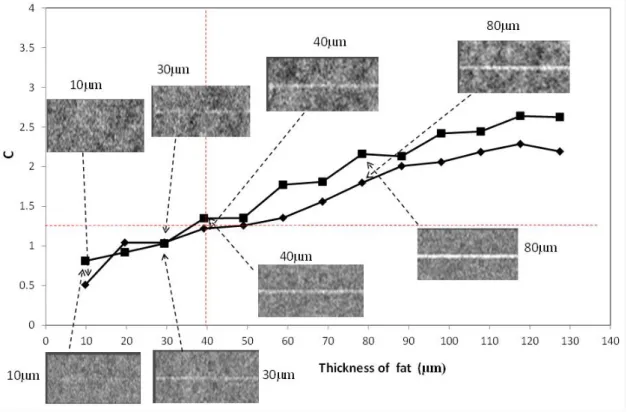
As stated in the previous section we determined a threshold on the contrast under which fat layers could not be distinguished. This led us to use this criterion to determine the thinnest fat layer that can be visualised. We considered here that the reference signals were perfectly known. Similar virtual objects as those described in section 2.5 were used for this part of the study. We simulated fat layers of from 10 to 130 m by step of 10m both at the beginning and at the end of the proving.

Figure 15 presents the variation of 𝐶𝑁𝑅_𝑓 in function of the thickness of the fat layer together with a selection of maps of fat proportions. In these maps, black is used for the minimum value, white for the maximum value, and grey levels varying linearly/proportionally to the fat proportions in between. A fat layer was easier to distinguish when 𝐶𝑁𝑅_𝑓 increased. There was a slight difference in detectability, i.e. when 𝐶𝑁𝑅_𝑓 > 1.25, between the beginning and the end of proving, because the contrast between paste and fat increased during proving since the fat signal increases with the temperature while the dough signal decreases (the paste signal does not vary with temperature and the amount of gas drastically increases from 20 to 80%). We considered that the layers between 40 and 50 µm thick could be detected with the naked eye at the beginning of proving, and between 30 and 40 µm at the end. The single value of 40 µm was retained in the subsequent analysis.

4 Performance of the method assessed on genuine MRI images of Danish paste

We also tested the method on genuine MRI images of Danish paste. The validation on products like Danish paste is not as straightforward as that on virtual images of the preceding section since it is not possible to know the ground-truth in each voxel of the images. However, it is possible to validate the conservation of fat and paste amounts at the product scale, which gives an indication of global performance of the mapping method. Results on structural elements visualized in genuine images will be discussed in another paper (Deligny, Collewet, & Lucas, 2016).

4.1 Preparation of Danish paste samples

The procedure for preparing the laminated paste was previously reported in (Deligny & Lucas, 2015). Four and 8 fat layers were obtained by two-fold turns applied twice and three times, respectively. Twelve fat layers were obtained by a three-fold turn applied to a paste sheet with 4 fat layers.

Just before proving inside the MRI probe, optical fibers were placed in the Danish paste sample (10 cm×5 cm) and the atmosphere of the MRI device was controlled at 30°C (±1°C) under humidity close to saturation. Optimal proving duration for this recipe was 180 min accordingly to industrial practices; proving was prolonged for the interest of the study. Further details about the MRI device can be found in (Lucas, et al., 2010). Temperature was measured with pre-calibrated optical fibers (type T, 1 mm thick), and recorded every 10 s during proving using a data acquisition Luxtron 790 connected to a PC.

The MRI protocol described in section 2.3 was used. The whole experiment was repeated 3 times for each number of fat layers.

4.2 Estimated maps of fat proportion

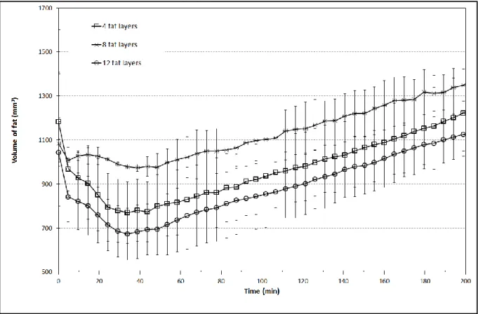
The volume of fat was not expected to change during proving, with the exception of some leakage at the edges of Danish paste. This was the first point in the verification of the method on genuine images of Danish paste. The estimated fat proportions calculated in all voxels belonging to the Danish paste sample (determined as described in section 2.4.2) were therefore added together. Only the slices (#3, 4, 5 and 6) in the most homogeneous area of the coil (see section 2.4.3) were considered for this analysis.

A decrease in fat volume (of at most 36%) was recorded during the first 40 minutes of proving, followed by an increase (Fig 16).

On the one hand, the decrease in total fat proportion was attributed to the uncertainty of the temperature in the Danish paste which propagated through estimation of the reference signal of fat. Indeed, the temperature measurements showed that 70% of the total temperature amplitude (10°C out of 14°C) between the sample and the proving atmosphere was attained within 35-40 min (Fig 4).

On the other hand, the simulation study on a proving fat-free dough (section 3.1.2 and Figure 9) showed an increase in the estimated fat quantity (from zero), hence a bias assignable to the method of quantification itself. The amplitude of increase was the same as observed in the present experiment. This meant in the case of Danish paste that the method most plausibly generated a positive bias for fat in the dough layers of the Danish paste.

Moreover, pure fat used in the calibration procedure mentioned above may differ from the fat material incorporated in the paste after lamination, because of the application of pressure forces. And the consequent structural changes in fat may impact the MRI signal:

- modification of the network of fat crystals and subsequently relaxation times of the liquid phase in the present case; such changes were recently characterized on pure triglycerides (Adam-Berret, Riaublanc, & Mariette, 2009) but not on mixtures of fatty acids to date. In this context, this effect could not be further discussed.

- modification of the solid fat content, under pressure or temperature (shear) increase; a recrystallization process with possible supercooling is also expected at the cooling steps managed between repeated sheetings. Lamination applied to Danish paste was also applied to pure fat, and solid fat content was measured by NMR (ISO 8292-1:2008). Deviation from the liquidus curve in the phase diagram was less than 1% at the end of sheeting (15°C) (data not shown). In such conditions, equilibrium was re-established at 16°C, well before placing the sample in the MRI proving chamber (starting from 19.5°C, see Fig 3). This effect could hence be neglected.

To conclude this experimental verification step, the maps of fat proportion were not accurately estimated and the error could be mainly attributed to the dough layers in which an increasing proportion of fat is “created” as shown in the simulation study. Likewise, this study has also shown that the bias of fat proportion in a voxel containing fat was, in the contrary, very low, smaller than 1%. Thus, localized measurements around

fat layers in the Danish paste, which involves voxels with moderate to high fat content, could be considered as reliable for further analysis.

4.3 Estimated maps of gas proportion

Concerning the estimated gas proportions, our approach was to check if the total volume of gas in Danish paste deduced from the maps of gas proportion (noted 𝑉_𝑔𝑡𝑝𝑟𝑜𝑝) was equal to 𝑉_𝑔𝑡𝑠𝑢𝑟𝑓, the total volume of gas calculated from the variations in the total area of the Danish paste cross-section as observed in the MRI images.

𝑉_𝑔𝑡𝑠𝑢𝑟𝑓 is provided by:

𝑉_𝑔𝑡𝑠𝑢𝑟𝑓= 𝑛_𝑡∆𝑉 − (1 − 𝑝̅𝑔0)𝑛0∆𝑉 (18)

where ∆𝑉 is the voxel volume, p̅_g0 the mean proportion of gas in the Danish paste sample at t = 0, which is supposed to be equal to 0.3 (see Fig 3 at t = 0). 𝑛𝑡 represents the number of voxels belonging to the paste at time 𝑡 and is measured as described in section 2.4.2. In the right-hand term of Equation (18), the first group is the volume of the sample at time t, and the second the volume of paste estimated from the volume of Danish paste at t = 0 and the knowledge of the gas proportion at that time.

On the other hand, the total volume of gas deduced from the maps of gas proportion V_gtprop is provided by: 𝑉_𝑔𝑡𝑝𝑟𝑜𝑝= ∑ 𝑝_𝑔𝑥𝑡

𝑥 ∈𝑀𝑡

∆𝑉 ₍₁₉₎

Fig 17 represents 𝑉_𝑔𝑡𝑝𝑟𝑜𝑝 as a function of 𝑉_𝑔𝑡𝑠𝑢𝑟𝑓. A systematic error of 5% was found, thus confirming the high level of accuracy of the method for estimating the gas proportion in Danish paste. The same level of error was previously estimated on virtual images where a bias was observed (see section 3.1.1 and Figure 8 ) This result confirmed the major working hypotheses or approximations on which the method was based, among them: the constancy of the reference signal of paste (section 2.4.2) and the omission of spatial inhomogeneities (section 2.4.3).

5 Conclusion

We developed a method to estimate the proportion of the components included in each voxel of a MRI image and this was applied to the characterization of Danish pastries during proving. The method was based on the modelling of the signal as a sum of the signal of each component weighted by their proportion. The estimated proportions were those which minimized a function that was the sum of the squared difference between the data and the model and a regularization that ensured the smoothness of the solutions. It required the a priori knowledge of two reference signals (fat and paste). The noise in MRI is Rician, however the method was based on the hypothesis of a Gaussian noise.

The choice of the parameters of the algorithm that set the weight of the regularization term in the criterion was determined using simulated images. Using these parameters, and assuming excellent estimations of the reference signals, we showed that, in the case of our application, the mean error (systematic bias) was similar with or without regularization and depended on the components and their proportion while the dispersion of these errors was much lower with regularization, consistently with the known function of regularization to remove noise. Fat and gas proportions were overestimated while paste proportion was underestimated. The absolute values of the bias varied from less than 1% up to 6% depending on the component and on the time of proving. The errors were larger for high gas proportion, i.e. at the end of the proving because of the lower 𝑆𝑁𝑅. The standard deviation of the errors varied from 0.3% up to 1.5 %. These values are not very high and acceptable for the targeted application.

Monte-Carlo simulations showed that these results were not influenced very much by the uncertainty on the reference signals at the end of the proving. However larger uncertainties were found at the beginning of

proving due to the values of the reference signals of fat. Indeed, at this stage of proving they were lower, decreasing the contrast between fat and paste, and they were also more sensitive to the value of the temperature. We computed the contrast-to-noise ratio and found that it was higher with regularization no matter the proving time. We showed that the regularization of the solutions did improve the visualization of the structures confirming the interest of this approach.

We also found that layers down to 40 m thick and bubbles of which size exceeded 2.5mm could be easily distinguished in fat and gas proportion maps respectively.

Finally, experiments on genuine MRI images of Danish paste (prepared with 4, 8 and 12 fat layers) confirmed the results obtained with the simulation study. We were able to validate the method at the scale of the Danish paste by observing the evolution of the sum of the fat proportion over time, as well as the evolution of the gas content compared with the evolution of the size of the pastry. This confirmed the possibility to use the method to study the proving of a Danish paste.

6 References

Adam-Berret, M., Riaublanc, A., & Mariette, F. (2009). Effects of Crystal Growth and Polymorphism of Triacylglycerols on NMR Relaxation Parameters. 2. Study of a Tricaprin-Tristearin Mixture. Crystal

Growth & Design, 9 (10), 4281-4288.

Artz, N. S., Hines, C. D. G., Brunner, S. T., Agni, R. M., Kuhn, J. P., Roldan-Alzate, A., . . . Reeder, S. B. (2012). Quantification of Hepatic Steatosis With Dual-Energy Computed Tomography Comparison With Tissue Reference Standards and Quantitative Magnetic Resonance Imaging in the ob/ob Mouse. Investigative Radiology, 47 (10), 603-610.

Babin, P., Della Valle, G., Chiron, H., Cloetens, P., Hoszowska, J., Pernot, P., . . . Dendievel, R. (2006). Fast X-ray tomography analysis of bubble growth and foam setting during breadmaking. Journal of

Cereal Science, 43 (3), 393-397.

Bajd, F., & Sersa, I. (2011). Continuous monitoring of dough fermentation and bread baking by magnetic resonance microscopy. Magnetic Resonance Imaging, 29 (3), 434-442.

Bellido, G. G., Scanlon, M. G., Page, J. H., & Hallgrimsson, B. (2006). The bubble size distribution in wheat flour dough. Food Research International, 39 (10), 1058-1066.

Bonny, J. M., Rouille, J., Della Valle, G., Devaux, M. F., Douliez, J. P., & Renou, J. P. (2004). Dynamic magnetic resonance microscopy of flour dough fermentation. Magnetic Resonance Imaging, 22 (3), 395-401.

Cauvain, S. P., & Telloke, G. W. (1993). Danish pastries and croissants (Vol. FMBRA Report No. 153). Chipping Campden, UK: CCFRA.

Cauvain, S. P., Whitworth, M. B., & Alava, J. M. (1999). The evolution of bubble structure in bread doughs and its effect on bread structure. In G. M. Campbell, C. Webb, S. S. Pandiella & K. Niranjan (Eds.),

Bubbles in Food (pp. 85-93). St Paul, Minnesota, USA: Eagan Press.

Chan, T. F., & Vese, L. A. (2001). Active contours without edges. Ieee Transactions on Image Processing,

10 (2), 266-277.

Collewet, G., Bugeon, J., Idier, J., Quellec, S., Quittet, B., Cambert, M., & Haffray, P. (2013). Rapid quantification of muscle fat content and subcutaneous adipose tissue in fish using MRI. Food

Chemistry, 138 (2-3), 2008-2015.

Deligny, C., Collewet, G., & Lucas, T. (2016). Spatial distribution of fat and gas in Danish paste during proving, with focus on structural elements as bubbles and layers. submitted to Food Research

International.

Deligny, C., & Lucas, T. (2015). Effect of the number of fat layers on expansion of Danish pastry during proving and baking. Journal of Food Engineering, 158, 113-120.

Filloux, A. M. (2008). Evaluation de la qualité technologique d'une pâte feuilletée. IAA (janv-févr.), 22-27. Furnols, M. F. I., Teran, M. F., & Gispert, M. (2009). Estimation of lean meat content in pig carcasses using