Surface profile prediction and analysis applied to turning process

Science Arts & Métiers (SAM)

is an open access repository that collects the work of Arts et Métiers Institute of Technology researchers and makes it freely available over the web where possible.

This is an author-deposited version published in: https://sam.ensam.eu Handle ID: .http://hdl.handle.net/10985/8994

To cite this version :

Chen LU, Jean-Philippe COSTES - Surface profile prediction and analysis applied to turning process - International Journal of Machining and Machinability of Materials, - Vol. Vol. 4, n°2/3, p.158-180 - 2008

Any correspondence concerning this service should be sent to the repository Administrator : archiveouverte@ensam.eu

Surface profile prediction and analysis applied

to turning process

Chen Lu

Department of System Engineering of Engineering Technology, Beihang University, Beijing 100083, PR China Fax: +86-10-8231-6570 E-mail: luchen@buaa.edu.cn

Jean-Philippe Costes*

Rue Porte de Paris, Cluny 71250, France Fax: +33-385-595-370

E-mail: jean-philippe.costes@cluny.ensam.fr *Corresponding author

Abstract: An approach for the prediction of surface profile in turning process using Radial Basis Function (RBF) neural networks is presented. The input parameters of the RBF networks are cutting speed, depth of cut and feed rate. The output parameters are Fast Fourier Transform (FFT) vector of surface profile for the prediction of surface profile. The RBF networks are trained with adaptive optimal training parameters related to cutting parameters and predict surface profile using the corresponding optimal network topology for each new cutting condition. A very good performance of surface profile prediction, in terms of agreement with experimental data, was achieved with high accuracy, low cost and high speed. It is found that the RBF networks have the advantage over Back Propagation (BP) neural networks. Furthermore, a new group of training and testing data were also used to analyse the influence of tool wear and chip formation on prediction accuracy using RBF neural networks.

Keywords: surface; machining: turning; neural network.

Biographical notes: Chen Lu is an Associate Professor at the Institute of Reliability Engineering of Beihang University, China. He has done his PhD in Fault Diagnosis for Mechanism and Internal Combustion Engine. He holds a Postdoctoral position in Fault Diagnosis and Monitoring, Network-Based Systems. His main expertise is in distributed remote monitoring system for equipment, non-destructive evaluation, software development and testing and signal processing.

Jean-Philippe Costes is an Assistant Professor in Machining Science in ENSAM, Department of Machining in Cluny, France. He has done his PhD about High Speed Machining and Roughness of Generated Surfaces. His main expertise is in dynamics of machining process, roughness profile, process simulation and cutting forces. He has published in journals such as International Journal of Tool and Manufacture and Journal of

Wood Science.

1 Introduction

The surface profile and roughness of a machined part are two of the most important product quality characteristics. The surface finish profile of a machined workpiece is affected by cutting conditions (parameters), tool geometry, workpiece material and other factors such as tool wear and vibrations. Surface roughness is a widely used index of product quality and in most cases a technical requirement for mechanical products. Achieving the desired surface quality is of great importance for the functional behaviour of a part. The process-dependant nature of the surface profile and roughness formation mechanism along with the numerous uncontrollable factors that influence pertinent phenomena, make it almost impossible to find a straight-forward solution and an absolutely accurate prediction model.

The aim of this study is to only use cutting speed (vc), cutting depth (ap), feed rate (f)

and Radial Basis Function (RBF) neural networks to investigate the possibility of surface profile and roughness prediction with high speed, online and low cost.

2 Review of literature

A brief review of the present research on the prediction of surface roughness and profile is discussed based on the work that Benardos and Vosniakos (2003) have investigated.

The classification of current literature is not easy due to the reason that many papers combine and blend different methodologies into a single approach. Therefore, no single classification would be entirely accurate. Considering the above, three major categories are created to classify the approaches. These are:

1 pure modelling 2 signals plus modelling 3 Artificial Intelligence (AI).

Here, the selected representative papers are introduced as below. 2.1 Pure modelling

Grzesik (1996) used the minimum undeformed chip thickness to predict surface roughness in turning. The study (Baek et al., 2001) presented a surface roughness model for face-milling operations considering the profile and run out error of each insert. The modelling technique developed in Chen et al. (1998) could represent the spectrum of surface topography ranging over shape, waviness and roughness. A surface roughness,

waviness and shape error model was obtained by the B-spline curve fitting of regenerated roughness. Ehmann and Hong (1994) introduced a ‘surface-shaping system’, which modelled the machine tool kinematics and cutting tool geometry, to represent the surface generation process in the simulation of 3D topography of a peripherally milled surface. Feng and Wang (2002) included six parameters, namely the hardness, feed rate, tool point angle, depth of cut, spindle speed and cutting time to build a model for finishing turning operations. Feed rate was identified as the most important factor along with cutting time. The work in Fuh and Wu (1995) investigated the influence of tool geometry and cutting conditions on machined surface quality. Investigation of the above factors in relation to the residual stresses was also carried out. The innovation with the work was that Response Surface Methodology (RSM) and Taguchi method were combined.

Remark 1: These studies have simulated the cutting process in terms of kinematics, cutting tool properties and cutting parameters. Additional factors, such as cutting forces, vibrations, wear and deflection of the cutting tool or certain thermal phenomena were also included to more accurately depict the phenomenon. The drawbacks are that a lot of factors contributing to the roughness formation mechanism need to be considered and integrated for a high accuracy, and that it also need to solve and update those complicated mathematic equations that may not have a satisfactory accuracy under some circumstances.

2.2 Signal plus modelling-based approach It includes:

1 optics and computer vision

2 sound signal, Acoustic Emission (AE), ultrasound 3 vibration signal.

These approaches, based on cutting forces, sound and vibration, laser scanners, vision systems and computer tomography, have the merit of independence of complicated mathematic modelling. On the other hand, there are still some drawbacks: some signals may be redundant; measuring errors are not easy to be avoided, resulting in inaccurate prediction and measuring cost is relatively high.

2.2.1 Optics and computer vision

Lee and Tarng (2001) proposed the use of computer vision techniques to inspect surface roughness. A polynomial network using a self-organising adaptive modelling method was applied to the construction of relationship between the extracted feature of surface image and the actual surface roughness. An optical profilometer using lateral effect photodiode to measure the relative height of the surface was developed by Lemaster and Taylor (1999). Fuchs (1997) used the application of computer vision and pattern analysis for the inspection of wooden materials, such as X-ray Computed Tomography (CT). Faust (1987) correlated camera images with stylus tracing and visual classification. However, the inspection speed is constrained by the complexity of the computing algorithm. The high cost of devices and their sophisticated designs make them unsuitable for industrial real-time application.

2.2.2 Sound signal, ultrasound, AE

Mannan et al. (2000) proposed a surface texture analysis combining sensory data from image and sound analysis to investigate the correlation between tool wear and qualitative characterising machined surface and sound pattern. However, it could not give more quantitative prediction. Regarding the applications of ultrasound, there are few papers published. An ultrasound wave-based approach was conducted in Coker and Shin (1996) for in-process monitoring and control of surface roughness. An ultrasonic sensor connected to a PC, produced a pulse which was then reflected by the surface of workpiece and measured the amplitude of the returned signal. The main advantage is that it is not affected by cutting fluids and chips as is the difficulty of other in-process schemes. In Gui-jie et al. (2003), the online measuring of surface roughness was estimated by taking into account the power spectrum density of friction-induced AE. Diniz et al. (1992) conducted related experiments to monitor the change of surface roughness caused by the deterioration of tool wear, through the variation of AE in finish turning.

2.2.3 Vibrations plus modelling-based approach

Concerning vibration-based approach, most of published paper have incorporated modelling method or kinematics to obtain an accurate surface roughness evaluation.

Lin and Chang (1998) incorporated the effect of the relative motion between cutting tool and workpiece with the effects of tool geometry, cutting parameters to simulate the surface geometry. It was also found that the effects of the radial direction vibrations on the surface roughness were much more significant than those of either the tangential direction vibrations or the axial direction vibrations. In Jang et al. (1996), the relative vibrations between tool and workpiece were superimposed onto the kinematic roughness calculated by tool edge radius and feed rate. It was found that the surface roughness contained specific frequency components determined by feed marks in the lower frequency range, and closely related to the natural frequencies of spindle–workpiece system in the high frequency range.

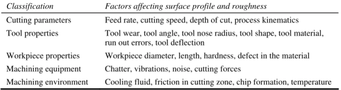
In Ghani and Choudhury (2002), the vibrations were used for monitoring tool wear and verifying the correlation between tool wear progression and surface roughness. In Abouelatta and Madl (2001), the cutting speed, feed rate, depth of cut, tool nose radius, tool overhang, approach angle, workpiece length and workpiece diameter and the vibrations in both radial and feed directions were used for evaluating tool life and surface roughness. Luo et al. (2003) presented a novel approach of surface quality evaluation by online vibration analysis and feature extraction using an adaptive B-spline wavelet algorithm. The results showed that the amplitude in the selective frequency bands and the root sum square of wavelet power spectrum reflected the surface quality. Remark 2: This is the most conventional experiment – observation – conclusion strategy. Its advantage lies in the fact that it is not difficult to implement. Regarding its disadvantages, the obtained conclusions have little or no general applicability. It must be pointed out that, it is very easy for an experiment to obtain the unexpected results since there are various errors in experimental environment. Here, all factors affecting surface quality are listed as in Table 1, mostly based on the review summarised by Benardos and Vosniakos (2003).

Table 1 Factors affecting surface profile and roughness

Classification Factors affecting surface profile and roughness

Cutting parameters Feed rate, cutting speed, depth of cut, process kinematics Tool properties Tool wear, tool angle, tool nose radius, tool shape, tool material,

run out errors, tool deflection

Workpiece properties Workpiece diameter, length, hardness, defect in the material Machining equipment Chatter, vibrations, noise, cutting forces

Machining environment Cooling fluid, friction in cutting zone, chip formation, temperature

2.3 AI approach

AI has been implementing in surface quality prediction through the development of Artificial Neural Network (ANN) models, Genetic Algorithms (GAs), fuzzy logic and knowledge-based expert systems, which simulate the way in which human beings process information and make decisions.

Risbood et al. (2003)used cutting speed, feed rate, depth of cut, radial components of cutting force and acceleration of radial vibration of tool holder to train different Back Propagation (BP) ANN models for the prediction of surface roughness and dimensional deviation for dry and wet turning, as well as for turning by HSS and carbide coated tools. Benardos and Vosniakos (2002) presented a BP ANN model trained with the Levenberg–Marquardt (L–M) algorithm for the prediction of surface roughness in face milling. The considered factors were depth of cut, feed rate, cutting speed, cutting forces, the engagement and wear of cutting tool, the use of cutting fluid. Ezugwu et al. (2005) developed a three-layered BP ANN model for the analysis and prediction of the relationship between cutting conditions and process parameters. The inputs of ANN were the cutting speed, feed rate, depth of cut, cutting time and coolant pressure. The outputs were tangential force, axial force, spindle motor power, machined surface roughness, average flank wear, maximum flank wear and nose wear. Azouzi and Guillot (1996) proposed an intelligent sensor fusion technique based on statistical tools and neural network to estimate surface finish and dimensional deviation. It was found that feed, depth of cut and radial force components provided the best average effect on surface quality. In Varghese and Radhakrishnan (1994), a sensor fusion approach incorporating ANNs was also described. The RMS value of the capacitive, inductive and fibre-optic sensors along with the type of manufacturing process were coded in binary format and then used to train an ANN. Mainsah and Ndumu (1998) developed an online ANN-based 3D surface characterisation/classification to place any new surface into its corresponding manufacturing process group and different roughness categories.

Some researchers also focus on the application of a knowledge-based extrapolation system for surface roughness prediction. Abburi and Dixit (2006) developed a knowledge-based system for the prediction of surface roughness in turning using neural network and fuzzy set theory. Knowledge obtained from the experiments was used to train the neural network that provided a number of data sets. All data sets were then imported into a fuzzy-set-based rule generation module to generate IF-THEN rules. Remark 3: It is obvious that the aforementioned ANNs approaches can produce very good results and simultaneously offer the possibility for online monitoring and/or control of the process.

Compared with classic programming, the main advantages of ANNs are:

1 there is no need to explicitly formulate the solution algorithm or to write code 2 the process of information is distributed over the neurons which operate in

parallel

3 models created by AI seem to be the most realistic and accurate, and this approach can be used in conjunction with other conventional techniques including signal analysis, kinematics, knowledge reasoning, etc. The most obvious drawbacks of the ANNs are:

1 a large number of experimental data sets are demanded for training a high accuracy of neural network

2 low generalisation ability markedly results in high errors for those inputs that are not in the range of training data set

3 network training easily falls into over-fitting area due to inappropriate training settings.

Optimisation of cutting parameters for a certain surface roughness is another focus that is being given more attentions. GA and other optimisation algorithms (simulated annealing, ANT algorithm, etc.) could be ideally used in conjunction with the developed models.

3 Description of prediction of surface profile and roughness using RBF ANN

In this study, an ANN modelling approach was developed for predicting surface profile and roughness. As the aforementioned, BP neural networks have been popularly used. However, BP algorithms have some inherent disadvantages, such as low rate of convergence, easily falling into local minimum point, weak global search capability, etc. Improved BP algorithms mainly introduce adaptive learning rate, momentum factor or train networks with gradient descent, quasi-Newton or resilient BP algorithm, etc. GA is also a good choice to search the optimal network topology. But BP ANNs still have some drawbacks that could not be avoided, such as low generalisation and over-fitting phenomena.

Considering the dynamic behaviour of machining process, the combination of cutting parameters and feature parameters extracted from vibrations and sound using Fast Fourier Transform (FFT) or wavelet, could give a reasonably accurate evaluation of machined surface roughness. The more the number of cutting parameters and feature vectors is, the higher the prediction accuracy will be. However, many random and experimental errors seem to be unavoidable when signals are measured. Furthermore, feature extractions need corresponding sensors including dynamometer of cutting force, piezoelectric accelerometer, acoustic sensor, eddy current displacement sensor, CCD camera, etc., resulting in the increase of measuring cost as well as the inconvenience of installing sensors under some environment. Due to the drawbacks of BP ANNs, other suitable ANNs should be recommended as complementary choices. In this study, Gaussian function-based RBF ANN was used, which has a higher performance over BP ANN. Cutting parameters (f, ap, v) were used to train network for the prediction of

3.1 The structure of RBF ANN for prediction of surface profile and roughness

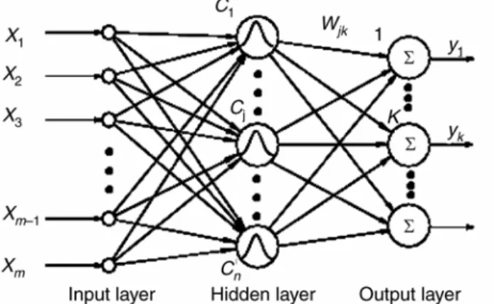
The suggested RBF ANN has an input layer, an output layer and a hidden layer composed of RBF neurons. The input space can be either an actual or a normalised representation. The network structure is shown in Figure 1. Here, inputs x1, x2,…, xm

composing an input vector x, are applied to all neurons in the hidden layer. The hidden layer is composed of n RBFs that are connected directly to all the elements in the output layer. Detailed descriptions of RBF networks can be found in Zhang and Zhang (2004), Park and Sandberg (1991), Bi et al. (2002) and Schalkoff and Robert (1997). A node in the hidden layer will generate a greater output when the input pattern is close to its centre. The output of such a node will decrease as the distance from the centre increases. Thus, for a given input pattern, only the neurons whose centres are close to the input pattern can generate non-zero activation values.

Figure 1 The structure of RBF neural network

The RBF for the jth hidden node is often defined by a Gaussian exponential function shown in Equation (1):

( )

where σ is the spread (width) of the jth corresponding Gaussian function. Usually the j

spread σ > should be not more than the possible maximum distance between the j( 0) input vector and the centre of the RBF, and it is determined by experiments. vjis defined

by the Euclidean norm of the distance between the input vector and the centre calculated as Equation (2):

(

)

∑

, Cj is the centre of the jth RBF unit, which has the same

The network output Y is formed by a linearly weighted sum of the RBFs in the hidden layer. The values for the output nodes can be calculated as

1 n k jk j j y w h = =

∑

where y_k is the kth element of the Y, is the output of the kth node in the output layer,

jk

w is the weight from the jth hidden layer neuron to the kth output layer neuron and hjis

the output of the jth node in the hidden layer. The transform from the input layer to the hidden layer is non-linear, and the output of the network is a linear combination of the RBFs computed by the hidden layer nodes.

3.2 RBF network training and testing

The RBF ANN has two operating modes, namely training and testing. Training an RBF network involves determining the number of RBFs, the corresponding centres and the output layer weight matrix. The criterion is to minimise the Sum of Squared Errors (SSE) defined as

( )

{

}

∑∑

t is each target value of the network output layer when the network is trained with input vector i

X , N is the number of training samples.

The details of the training procedure would be out of the scope of this paper, but could be found in other references. Once the centres and the widths (spreads) have been chosen, a supervised learning algorithm is applied to train the weights between the hidden and the output layer nodes. The output layer weights are usually trained using the Least Mean Squares (LMS) algorithm. In summary, there are basically three steps for creating a RBF network:

calculate the number n of the hidden layer

calculate the centres and the widths of the hidden layer determine the weights of the output layer.

When the above steps are completed, an RBF neural network is fully obtained. Then it can calculate the output result for each new input vector through Equations (1)–(3). 3.3 Comparison between RBF ANN and BP ANN

As multilayer feed-forward networks, RBF ANNs are superior to BP ANNs though the latter have been popularly applied (30–31). Generally, RBF ANNs store knowledge locally in neurons whereas BP ANNs globally. In RBF ANNs, the optimal number of hidden neurons can be obtained during the training process, however, for BP ANNs, the number of hidden neurons has to be prior determined before the training process, and it is also difficult to determine the optimal number of hidden neurons. In RBF ANNs, the maximum number of iterations cannot be more than the number of training samples and the output error reaches zero when the number of hidden neurons exceeds the number of

training samples. BP ANNs use gradient descent method to minimise the error and the error might converge very slowly, moreover, the residual error might be unacceptable. Furthermore, a BP ANN trained with same parameters at different time would always have different topologies due to its random initial weights and biases, resulting in different training and simulation results, but the RBF ANN does not have this drawback. Besides, BP ANNs might fall into a local optimum, which has to be given up. Compared with BP ANNs, RBF ANNs can be created rapidly with convergence and accuracy guaranteed. Consequently, RBF neural network models would be suitable for the surface profile and roughness prediction. A trained RBF network structure could also be quickly readjusted and retrained online for higher accuracy.

4 Experimental conditions and procedure 4.1 Experimental set-up and conditions

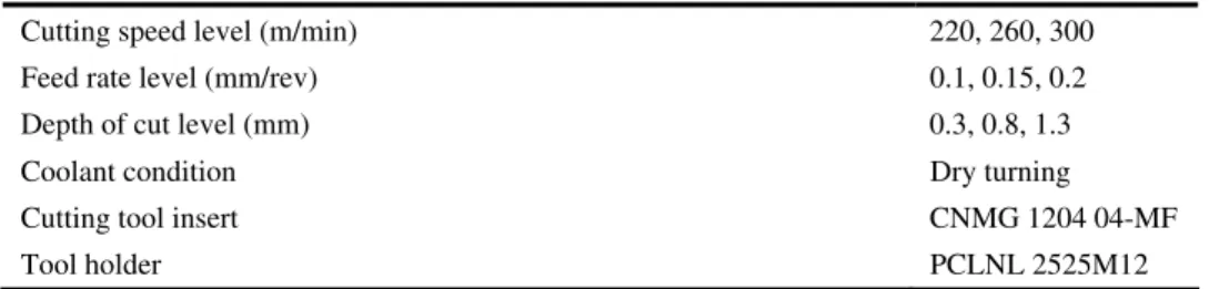
Machining tests were conducted on a CNC turning lathe. Stainless steel 304L with a diameter of 95.5 mm was used as workpiece. The workpiece was machined using carbide coated inserts CNMG120404-MF. Cutting conditions in the experiments are shown in Table 2. The experimental set-up is shown in Figure 2.

Table 2 Cutting conditions

Cutting speed level (m/min) 220, 260, 300

Feed rate level (mm/rev) 0.1, 0.15, 0.2

Depth of cut level (mm) 0.3, 0.8, 1.3

Coolant condition Dry turning

Cutting tool insert CNMG 1204 04-MF

Tool holder PCLNL 2525M12

Figure 2 Experimental set-up (see online version for colours)

For generating the training data for RBF neural networks, three levels of cutting speed, feed and depth of cut were taken as shown in Table 2. Thus 27 cases were combined into the training data set of RBF ANNs each case includes vc, ap, f and the measured

Table 3 Training data set for RBF neural networks

Case no. vc (m/min) ap (mm) f (mm/rev) R

a ( m) 1 220 0.3 0.1 0.612 2 220 0.3 0.15 1.195 3 220 0.3 0.2 1.606 4 220 0.8 0.1 0.547 5 220 0.8 0.15 1.583 6 220 0.8 0.2 1.998 7 220 1.3 0.1 0.563 8 220 1.3 0.15 1.004 9 220 1.3 0.2 1.268 10 260 0.3 0.1 0.636 11 260 0.3 0.15 1.183 12 260 0.3 0.2 1.581 13 260 0.8 0.1 0.871 14 260 0.8 0.15 1.705 15 260 0.8 0.2 2.160 16 260 1.3 0.1 0.655 17 260 1.3 0.15 1.010 18 260 1.3 0.2 1.269 19 300 0.3 0.1 0.634 20 300 0.3 0.15 1.194 21 300 0.3 0.2 1.469 22 300 0.8 0.1 1.100 23 300 0.8 0.15 1.645 24 300 0.8 0.2 2.185 25 300 1.3 0.1 0.623 26 300 1.3 0.15 0.983 27 300 1.3 0.2 1.327

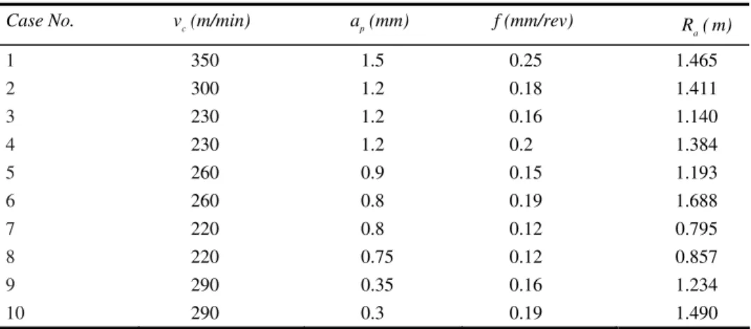
Additionally, 10 cases designed randomly within and outside the range of cutting parameter levels of training data set were employed as testing data set (Table 4). The testing data set did not participate in the training process (namely, not presented to the neural networks), but it was used to test the trained ANNs and search the optimal topology among different ANN topologies.

The machining length along the workpiece for each case was taken as 10 mm. The surface roughness of the machined workpiece was measured by a SOMICRONIC SURFASCAN S-M3 and a stylus with a radius of 10 µm, angle 60°. Readings were taken three times and the average value was recorded. The surface roughness evaluation length in each case was taken as 5.6 mm. Considering the influence of tool wear, the cutting tool insert was replaced by a new insert at No. 10, No. 19 for training data and at No. 6 for testing data, respectively, so the cutting tool insert was supposed not to be worn.

Table 4 Testing data set for prediction of surface profile and roughness

Case No. vc (m/min) ap (mm) f (mm/rev) R

a ( m) 1 350 1.5 0.25 1.465 2 300 1.2 0.18 1.411 3 230 1.2 0.16 1.140 4 230 1.2 0.2 1.384 5 260 0.9 0.15 1.193 6 260 0.8 0.19 1.688 7 220 0.8 0.12 0.795 8 220 0.75 0.12 0.857 9 290 0.35 0.16 1.234 10 290 0.3 0.19 1.490

4.2 Preparation and preprocessing of training data set 4.2.1 Construction of training data set

The prediction and generalisation capabilities of neural networks are essentially dependent on:

1 the selection of the appropriate input/output parameters

2 the training data set should be representative values for each input/output parameter

3 the distribution of the training data set

4 the format of the presentation of the training data set.

The aim of this research is to predict surface profile and roughness using RBF ANNs with the three main cutting parameters.

Both of the two tasks used the three cutting parameters (as shown in Table 3) to compose the input matrix (3 27× ) of a RBF ANN, namely, the number of nodes in the input layer was 3. For the prediction of surface roughness, Ra was taken as the output

vector (1 27× ) for each corresponding combination of cutting parameters, namely, the output layer has 1 node.

As for the prediction of surface profile, a new method to define the output matrix of a RBF ANN was tried, based on the method proposed by Poulachon et al. (1998). It is illustrated as following:

1 surface profile data measured by a stylus is first performed a 1024-point FFT 2 real and imaginary parts in the FFT complex vector are separated to construct a

new 2048 × 1 target (output) vector, in which the real part lies in the first 1024 elements and the imaginary part in the latter 1024 elements

3 the above steps are repeated for each profile in the training data set

4 after the training of the RBF network, each testing input vector is simulated, and a 2048 × 1 vector, which contains the real and imaginary parts of FFT predicted by the trained RBF network, is output

5 perform an inverse FFT (iFFT) to reconstruct the output profile, which is actually a transform form spatial-frequency domain to spatial domain.

In this experiment, each 2048 × 1 FFT target (output) vector of 27 training cases, together with the corresponding 3 × 1 input vector were used to train a RBF network for the prediction of surface profile. For the surface profile prediction, the training data set was composed of the 3 × 27 input matrix and 2048 × 27 target (output) matrix. For the surface roughness prediction, the training data set was composed of the 3 × 27 input matrix and 1 × 27 output matrix.

4.2.2 Normalisation of training data set

Prior to training the network, the input P and target T were normalised within the range of ±1, using the function [pn, minp, maxp, tn, mint, maxt] = premnmx(P, T) in Matlab. The algorithm is as below:

2 ( min ) 1 (max min ) P P pn P P × − = − − (5) 2 ( min ) 1 (max min ) T T tn T T × − = − − (6)

However, for the prediction of surface profile, premnmx is not suggested to normalise the 2048 × 27 target matrix. It was found that, the mints were equal to maxts in several lines of matrix T, which resulted in a zero value in denominator. The reason should be that, the 27 values in several lines were the same after FFT transform, namely, the real parts or imaginary parts were the same at some spatial frequency locations. Therefore, a global mint and maxt of the whole matrix T (FFT matrix) were employed, not from each line of T. Then, the normalised values were calculated using Equation (6).

4.3 Training and parameter optimisation for RBF neural networks

The training and simulation were conducted using the neural network functions in Matlab (Anonymous, 2006), which include newgrnn ( ), newrbe ( ), sim ( ) and mse ( ). The data acquired from the turning process was divided into the training data set comprising 27 cases and the testing data set comprising 10 cases.

4.3.1 Training for surface profile and roughness

It was found that newgrnn ( ) and newrbe ( ) are suitable for the prediction of surface profile and roughness, respectively, each of which can obtain a satisfactory prediction result. Furthermore, compared with BP neural networks, RBF neural networks self-adaptively add the number of neurons in hidden layer until the error goal is met.

newgrnn ( ) was used in the training of RBF network for the prediction of surface roughness.

net = newgrnn(P, T, spread), designs a generalised regression neural network. Where P, T, spread and net are matrix of input vectors, matrix of target vectors, spread of RBFs and returned network structure, respectively. Generalised regression neural networks are a kind of radial basis network that can be used for function approximation between the three cutting parameters and predicted surface roughness. The larger that spread is, the smoother the function approximation will be. To fit data closely, use a spread smaller than the typical distance between input vectors. To fit the data more smoothly use a larger spread.

newrbe ( ) was used in the training of RBF network for the prediction of surface profile.

net = newrbe(P, T, spread). Where P, T and spread, net are input vector, target vector, spread of RBF and returned network structure, respectively. The newrbe very quickly designs an exact radial basis network with zero error.

4.3.2 Simulation and testing of a trained RBF neural network

Function Yt = sim(net, pt); where pt, Yt are the input and simulated result of testing data set, respectively.

4.3.3 Performance evaluation

The performance of a RBF network, namely generalisation ability for testing data set outside the range of training data set, can be evaluated using Mean Squared Error (MSE). Suppose, Z = Yt − Y, the MSE is calculated by function mse(Z) in Matlab. The smaller the return value is, the better the generalisation ability of a trained neural network is.

4.3.4 Searching and determination of optimal training parameters

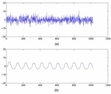
It has been found that, a RBF network trained with different spread values always returns different performances. Figure 3(a) is the measured profile with vc = 260, ap = 0.8,

f = 0.19 which lies in the testing data set in Table 3, Figure 3(b) is the surface profile predicted by a RBF network trained with spread = 0.14 and Figure 3(c) is the surface profile predicted by a RBF network trained with a default spread = 1. It is shown that Figure 3(b) has a better correlation with the measured profile than Figure 3(c), and that the spread parameter, which is used in the training of the RBF network, can significantly influence the trained network on the accuracy of prediction and generalisation ability.

Therefore, prior to determining the final spread for the training of a RBF network, it is suggested to train the RBF network with different spreads to find the optimal spread for the testing data set. In this experiment, the testing data set (Table 4) was used to evaluate the performance of all candidate networks trained with different spreads, and find out the optimal network with the least MSE.

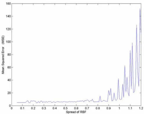
A total of 116 RBF network topologies were trained using the training data set (Table 3) and 116 different spreads ranging from 0.05 to 1.2 with a step of 0.01, then sim( ) and mse( ) were employed to evaluate the prediction performance for the given testing data set. 116 MSE values between the predicted and measured profiles for the whole testing data set were obtained respectively, as shown in Figure 4. It can be seen that the optimal spread value was 0.16 and the corresponding MSE was 4.3904, namely, when the training parameter spread was 0.16, the trained RBF network could give the least prediction error for the whole testing data set.

Similarly, for the prediction of surface roughness, the same approach was applied to search an optimal spread of newgrnn. The optimal spread value was found to be 0.78 at which the MSE was 0.0128, and the correlation coefficient between the predicted and measured roughness was 0.976.

Figure 3 Simulation of surface profile: (a) measured profile, (b) predicted profile, spread = 0.14 and (c) predicted profile, spread = 1 (see online version for colours)

4.3.5 Online retraining and readjusting of RBF network using a dynamic spread

However, for the prediction of surface profile, the aforementioned spread was only a global optimal value for the whole testing data set. It might not be a local optimal value for each case within the testing data set. It was found that, for some cases, the best correlation of profile shape and amplitude between the measured and predicted profiles were attained using the RBF network trained at a spread value near 0.16, such as 0.15, 0.135, etc. Therefore, the determination of local optimal spread value needs a coarse- and fine-adjusting procedure, and it should take into account not only MSE performance but also the correlation degree of shape and amplitude.

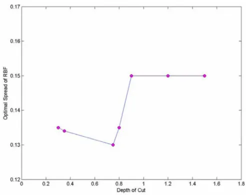
It was also found that, for each case in the testing data set, the depths of cut (ap) were

significantly related to the local optimal spreads. Namely, ‘a RBF network trained with a fixed spread parameter would not guarantee the optimal prediction or best generalisation ability for all profile prediction cases’.

It is suggested that, at each new prediction, the RBF network trained by prior optimal spread parameter should be online retrained and updated using a new optimal spread training parameter for high accuracy. The new optimal spread can be found from the correlation mapping between ap and optimal spread values. In this experiment,

under the specified machine, workpiece, cutting conditions as shown in Table 2, for the given training and testing data sets in Tables 3 and 4, the correlation mapping between ap

and optimal spreads was established for online retraining a RBF neural network, as shown in Figure 5.

Figure 5 Correlation between depth of cut and corresponding optimal spread (see online version for colours)

The online retraining of a RBF neural network using a dynamic spread parameter can be summarised as the following steps:

1 Suppose, there is a new given case (vc, ap, f) to be predicted its surface profile.

2 Select an appropriate optimal spread value according to the correlation mapping. Then, train a RBF network using the optimal spread parameter and the original training data set.

3 Once the training goal is met, dynamically update the RBF network with the new weights and biases and then simulate (predict) the given case, obtaining the predicted surface profile.

4 The procedure is repeated for any new case. Since a RBF network designs and creates a new topology very quickly, it is very feasible to online retrain a RBF network and predict.

5 Results and discussion

Ten cases of testing data set were used to evaluate the two RBF neural networks that performed the prediction of surface profile and roughness, respectively.

5.1 Experimental results of surface profile prediction

Due to limit of pages, part of 10 predictions of surface profiles is shown from Figures 6 to 8. The corresponding cutting condition, the MSE between the predicted profile and the measured profile are given, and the spread which was selected adaptively for each profile prediction is also listed as below. In each figure, the horizontal axes denotes the 1200 data points along the axial direction of workpiece surface and the vertical axes is the amplitude values of surface profile.

Figures 6–8 show that the predicted profiles have a good correlation with the measured profiles in terms of profile shape, trend and amplitude range. After selecting an appropriate optimal spread value, each testing profile was predicted using the RBF neural network trained with this spread. The MSE value in each testing case might not be the least value, however, the corresponding spread is just the optimal training parameter and the corresponding predicted profile has the best correlation with the measured actual profile than those spreads with other MSEs.

From the results, it is found that, the predicted profiles are still at small variance with the measured profiles in terms of amplitude, shape and initial phase consistency. The reason should be the presence of a lot of disturbing factors in the turning process, the factors might involve stochastic vibrations of spindle–workpiece, vibrations of lathe, vibrations of tool holder, chatter phenomena of lathe, disturbance of chip formation, etc.

More ANN input parameters, extracted from sensors of cutting forces, vibrations of spindle–workpiece, displacement signals of tool holder, etc., should theoretically improve the accuracy degree of surface profile prediction. Moreover, spatial frequency domain (wavelet or wavelet packet) information extracted from those signals might be an ideal approach to adjust the initial phase position. However, the above improvement would increase not only the cost of measuring systems but also the complexity that might import other noises and experimental errors, as well as influence the online prediction speed due to the task of signal processing.

Figure 6 (a) Predicted profile and (b) measured profile (vc = 220, ap = 0.8, f = 0.12,

MSE = 2.2616, spread = 0.133) (see online version for colours)

Figure 7 (a) Predicted profile and (b) measured profile (vc = 230, ap = 1.2, f = 0.2,

Figure 8 (a) Predicted profile and (b) measured profile (v_c = 260, a_p = 0.8, f = 0.19,

MSE = 17.7826, spread = 0.14) (see online version for colours)

These same surface profiles were also predicted by a trained BP neural network for comparing the performance with the well-trained RBF neural network. A number of BP network topologies with different training parameters and weights were tried for searching a topology that could provide minimum error. Finally, an improved BP network with 2 hidden layers and 10 neurons in each hidden layer, 3 input neurons and 2048 output neurons (3–10–10–2048), trained with {traingdx, learngdm} and {learning rate: 0.05, momentum: 0.9, minimum gradient:1e-20}, was chosen as the optimal network to predict the surface profiles. The tangent sigmoid transfer function ‘tansig’ and linear transfer function ‘purelin’ were used in the hidden and output layers, respectively. Figure 9 shows the predicted profile by the selected BP network for one case in the testing data set. Figure 9(a) is the predicted profile and Figure 9(b) is the measured actual profile under v_c = 260, ap = 0.8, f = 0.19.

It is evident from Figure 9 that the profile predicted by the BP network contains a lot of chaotic noises and severely distorted from the actual surface profile. It is also concluded that a BP network does not suit such a prediction involving a large number of output nodes (2048), and that a complicated BP network topology could lead to low generalisation capability and easily falling into over-fitting.

It was also found that compared with the RBF network, the search procedure for the optimal BP network topology took a very long time. Under a PC simulation platform of 1.6 GHz CPU with a memory size of 512 M, for BP neural network, it took about 1900 sec to obtain the best one from 30 BP topologies, whereas RBF network took only about 7 sec to reach the best one from 116 candidates. Therefore, it is proved that RBF neural network is very competent for the surface profile prediction that demands high-dimensional output vector (neurons) and has a significant advantage over BP network.

Figure 9 Surface profile under vc = 260, ap = 0.8, f = 0.19 predicted with BP network:

(a) predicted profile and (b) measured profile (see online version for colours)

5.2 Experimental results of surface roughness prediction

The results of surface roughness prediction for the testing data set (Table 4) are shown in Table 5. Here, the results predicted by the RBF network are compared with those predicted by a Conventional Mathematic Equation (‘CME’ used in the following) used in surface roughness calculation (as shown in Equation (7)) and a selected BP neural network. 2 a 18 3 f R Rε ≈ (7)

where Ra denotes surface roughness, f is feed rate, Rε is the radius of tool nose, here it is

0.4 mm.

Similarly, a BP neural network was also trained to predict the surface roughness. The optimal BP network was obtained from 200 candidate topologies with 2 hidden layers and 10 or 15 neurons in the hidden layers according to minimum MSE and maximum correlation coefficient (calculated by ‘postreg’ in Matlab) between the measured and the predicted roughness. The surface roughness was predicted using a 3–10–10–1 BP network trained by L–M algorithm with ‘tansig’ and ‘purelin’ transfer functions in the hidden and output layers, respectively.

Due to the aforementioned shortcomings of BP networks, it is actually easy to fall into a local optimal topology instead of the global optimal one. Contrary to RBF neural networks, a BP network trained with same parameters at different time would give

different outputs for same input vector since the initial weights and biases are random. Therefore, once a BP optimal topology is reached, it should be better to save the corresponding network topology including initial weights and biases for the subsequent predictions. The selected BP network might not be a global optimal, however, a global searching of BP would result in a huge searching spaces as well as block a desired fast speed on building ANN model. Consequently, it is suggested that RBF network should be adopted in high priority.

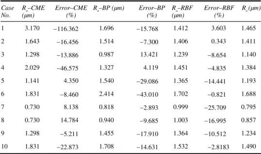
Table 5 Surface roughness predicted by RBF, BP and conventional mathematic equation

Case No. R_a–CME (µm) Error–CME (%) R_a–BP (µm) Error–BP (%) R_a–RBF (µm) Error–RBF (%) R_a (µm) 1 3.170 _−116.362 1.696 _−15.768 1.412 3.603 1.465 2 1.643 _−16.456 1.514 _−7.300 1.406 0.343 1.411 3 1.298 _−13.886 0.987 13.421 1.239 _−8.654 1.140 4 2.029 _−46.575 1.327 4.119 1.451 _−4.835 1.384 5 1.141 4.350 1.540 _−29.086 1.365 _−14.441 1.193 6 1.831 _−8.460 2.414 _−43.010 1.702 _−0.821 1.688 7 0.730 8.138 0.818 _−2.893 0.999 _−25.709 0.795 8 0.730 14.784 0.940 _−9.685 1.003 _−16.995 0.857 9 1.298 _−5.211 1.455 _−17.910 1.364 _−10.512 1.234 10 1.831 _−22.873 1.708 _−14.631 1.532 _−2.8183 1.490

In Table 5, Ra, Ra–RBF, Ra–BP, Ra–CME are the measured actual surface roughness

and the surface roughness predicted by the RBF network, BP network and CME, respectively. Error-RBF, Error-BP and Error-CME are respectively their corresponding percentage errors in the prediction. It can be seen that, compared with the other two methods, the RBF network could give the least degree of prediction error and the CME produces relatively high errors due to its simple model.

Table 5 shows that, in nine cases, the error in RBF-based prediction is less than 20%. Only in one cases, error is more than 20%, with a maximum error of −25.709%. The MSE of the whole testing data set predicted by the RBF network is 0.0128. It is considered that less than 20% error is reasonable, considering the inherent randomness in metal cutting process. Figure 10 shows the measured actual surface roughness versus the predicted surface roughness using RBF network. A line inclined at 45° and passing through the origin is also plotted in the figure. For perfect prediction, all points should lie on this line. Here, it can be seen that most of the points are close to this line. The correlation coefficient between the predicted roughness of the RBF network and the measured actual roughness is 0.976. Hence, this RBF neural network provides reliable prediction and high accuracy.

Figure 10 Correlation between the surface roughness predicted by the RBF network and measured actual surface roughness (see online version for colours)

6 Conclusions

The conclusions drawn from this paper can be summarised in the following points: 1 The RBF neural network trained by newrbe with adaptive-adjusting spreads

for different depths of cut was found to be the optimal network for the prediction of surface profile.

2 The correlation between spread and depths of cut was also established to online adjust the training parameters for different cutting conditions. The shape, amplitude and trend of surface profile machined by turning process could be predicted with a good consistency with the actual profile.

3 The RBF neural network trained by newgrnn with a searched optimal spread of 0.78 was found to be the optimal network for the prediction of surface roughness, with a high accuracy degree and correlation coefficient.

4 Compared with an improved BP neural network, the RBF neural network is suitable for the prediction of surface profile with a markedly high accuracy degree and fast prediction speed.

5 Concerning the prediction of surface roughness, the RBF network still has the significant advantage over a BP network and the CME.

6 Generally, the developed RBF network models based on the three cutting parameters (vc, ap, f) can realise the prediction of surface profile and roughness

with high accuracy, low-cost, high speed in turning process.

7 Based on the reviews of the published research works and the research in this paper, it is evident that ANNs are a powerful tool, easy-to-use and have a good prospect for the future applications.

References

Abburi, N.R. and Dixit, U.S. (2006) ‘A knowledge-based system for the prediction of surface roughness in turning process’, Robotics and Computer Integrated Manufacturing, Vol. 22, pp.363–372.

Abouelatta, O.B. and Madl, J. (2001) ‘Surface roughness prediction based on cutting parameters and tool vibrations in turning operations’, Journal of Materials Processing Technology, Vol. 118, pp.269–277.

Anonymous (2006) The MathWorks-Online Technical Documentation, Available at: http://www.mathworks.com/access/helpdesk/help/helpdesk.shtml.

Azouzi, R. and Guillot, M. (1996) ‘On-line prediction of surface finish and dimensional deviation in turning using neural network based sensor fusion’, International Journal of Machine Tools

and Manufacture, Vol. 37, No. 9, pp.1201–1217.

Baek, D.K., et al. (2001) ‘Optimization of feedrate in a face milling operation using a surface roughness model’, International Journal of Machine Tools and Manufacture, Vol. 41, pp.451–462.

Benardos, P.G. and Vosniakos, G.C. (2002) ‘Prediction of surface roughness in CNC face milling using neural networks and Taguchi’s design of experiments’, Robotics and Computer

Integrated Manufacturing, Vol. 18, pp.343–354.

Benardos, P.G. and Vosniakos, G.C. (2003) ‘Predicting surface roughness in machining: a review’,

International Journal of Machine Tools and Manufacture, Vol. 43, pp.833–844.

Bi, T., et al. (2002) ‘On-line fault section estimation in power systems with radial basis function neural network’, Electrical Power and Energy Systems, Vol. 24, pp.312–328.

Chen, C.C.A., et al. (1998) ‘A surface topography model for automated surface finishing’,

International Journal of Machine Tools and Manufacture, Vol. 38, pp.543–550.

Coker, S.A. and Shin, Y.C. (1996) ‘In-process control of surface roughness due to tool wear using a new ultrasonic system’, International Journal of Machine Tools and Manufacture, Vol. 36, pp.411–422.

Diniz, A.E., et al. (1992) ‘Correlating tool life, tool wear and surface roughness by monitoring acoustic emission in finish turning’, Wear, Vol. 152, pp.395–407.

Ehmann, K.F. and Hong, M.S. (1994) ‘A generalized model of the surface generation process in metal cutting’, CIRP Annal, Vol. 43, pp.483–486.

Ezugwu, E.O., et al. (2005) ‘Modelling the correlation between cutting and process parameters in high-speed machining of Inconel 718 alloy using an artificial neural network’, International

Journal of Machine Tools and Manufacture, Vol. 45, pp.1375–1385.

Faust, T.D. (1987) ‘Real time measurement of veneer roughness by image analysis’, Forest

Products Journal, Vol. 37, No. 6, pp.34–40.

Feng, C.X.J. and Wang, X. (2002) ‘Development of empirical models for surface roughness prediction in finish turning’, International Journal of Advanced Manufacturing Technology, Vol. 20, pp.348–356.

Fuchs, S. (1997) ‘Opportunities of sensor techniques for inspection of wood materials and its impediments’, Proceedings of the 13th International Wood Machining Seminar, Vancouver, Canada, pp.289–298.

Fuh, K.H. and Wu, C.F. (1995) ‘A proposed statistical model for surface quality prediction in end milling of Al alloy’, International Journal of Machine Tools and Manufacture, Vol. 35, pp.1187–1200.

Ghani, A.K. and Choudhury, I.A. (2002) ‘Study of tool life, surface roughness and vibration in machining nodular cast iron with ceramic tool’, Journal of Materials Processing Technology, Vol. 127, pp.17–22.

Grzesik, W. (1996) ‘A revised model for predicting surface roughness in turning’, Wear, Vol. 194, pp.143–148.

Gui-jie, L., et al. (2003) ‘On-line measuring of ground surface roughness based on friction-induced acoustic emission’, Tribology, Vol. 23, pp.236–239.

Jang, D.Y., et al. (1996) ‘Study of the correlation between surface roughness and cutting vibrations to develop an on-line roughness measuring technique in hard turning’, International Journal

of Machine Tools and Manufacture, Vol. 36, pp.453–464.

Lee, B.Y. and Tarng, Y.S. (2001) ‘Surface roughness inspection by computer vision in turning operations’, International Journal of Machine Tools and Manufacture, Vol. 41, pp.1251–1263.

Lemaster, R.L. and Taylor, J.B. (1999) ‘High speed surface assessment of wood and wood-based composites’, Proceedings of the 14th International Wood Machining Seminar, Paris, France, pp.479–488.

Lin, S.C. and Chang, M.F. (1998) ‘A study on the effects of vibrations on the surface finish using a surface topography simulation model for turning’, International Journal of Machine Tools and

Manufacture, Vol. 38, pp.763–782.

Luo, G.Y., et al. (2003) ‘Surface quality monitoring for process control by on-line vibration analysis using an adaptive spline wavelet algorithm’, Journal of Sound and Vibration, Vol. 263, pp.85–111.

Mainsah, E. and Ndumu, D.T. (1998) ‘Neural network application in surface topography’,

International Journal of Machine Tools and Manufacture, Vol. 38, No. 5, pp.591–598.

Mannan, M.A., et al. (2000) ‘Application of image and sound analysis techniques to monitor the condition of cutting tools’, Pattern Recognition Letters, Vol. 21, pp.969–979.

Park, J. and Sandberg, I.W. (1991) ‘Universal approximation using radial basis functions network’,

Neural Computer, Vol. 3, pp.246–257.

Poulachon, G., et al. (1998) ‘Surface roughness modelling by superfinish turning with cutting edge’, Proceedings-Volume II of the 2nd International Conference on Integrated Design and

Manufacturing in Mechanical Engineering, Compiègne, France, pp.533–540.

Risbood, K.A., et al. (2003) ‘Prediction of surface roughness and dimensional deviation by measuring cutting forces and vibrations in turning process’, Journal of Materials Processing

Technology, Vol. 132, pp.203–214.

Schalkoff, R.J. (1997) Artificial Neural Networks, New York: McGraw-Hill.

Varghese, S. and Radhakrishnan, V. (1994) ‘A multi-sensor approach to in-process monitoring of surface roughness’, Journal of Materials Processing Technology, Vol. 44, pp.353–362. Zhang, A. and Zhang, L. (2004) ‘RBF neural networks for the prediction of building interference