What is the cost of low participation in French timber auctions?

HAL Id: hal-00670762

https://hal.archives-ouvertes.fr/hal-00670762

Submitted on 16 Feb 2012

HAL is a multi-disciplinary open access archive for the deposit and dissemination of sci-entific research documents, whether they are pub-lished or not. The documents may come from teaching and research institutions in France or abroad, or from public or private research centers.

L’archive ouverte pluridisciplinaire HAL, est destinée au dépôt et à la diffusion de documents scientifiques de niveau recherche, publiés ou non, émanant des établissements d’enseignement et de recherche français ou étrangers, des laboratoires publics ou privés.

Raphaële Préget

To cite this version:

Raphaële Préget. What is the cost of low participation in French Timber auctions?. Applied Eco-nomics, Taylor & Francis (Routledge), 2011, pp.1. �10.1080/00036846.2010.539546�. �hal-00670762�

For Peer Review

What is the cost of low participation in French Timber auctions?

Journal: Applied Economics Manuscript ID: APE-08-0734.R1 Journal Selection: Applied Economics Date Submitted by the

Author: 28-Sep-2010

Complete List of Authors: Préget, Raphaële; INRA, LAMETA JEL Code:

C11 - Bayesian Analysis < C1 - Econometric and Statistical Methods: General < C - Mathematical and Quantitative Methods, C34 - Truncated and Censored Models < C3 - Econometric Methods: Multiple/Simultaneous Equation Models < C -

Mathematical and Quantitative Methods, D44 - Auctions < D4 - Market Structure and Pricing < D - Microeconomics, L73 - Forest Products: Lumber and Paper < L7 - Industry Studies: Primary Products and Construction < L - Industrial Organization Keywords: timber auctions, hedonic prices, sample selection, endogenous

participation

For Peer Review

3 4 5 6 7 8 9 10 11 12 13 14 15 16 17 18 19 20 21 22 23 24 25 26 27 28 29 30 31 32 33 34 35 36 37 38 39 40 41 42 43 44 45 46 47 48 49 50 51 52 53 54 55 56 57 58

For Peer Review

What is the cost of low participation in French Timber auctions?

R. Prégeta,* _{and P. Waelbroeck}b

How much is the standing timber from public forests worth? To estimate the value of a timber lot we adopt the transaction-evidence appraisal approach using data from timber auctions in Lorraine (Eastern France) accounting for the facts that: (i) the seller’s reserve prices are secret, (ii) there remain many unsold lots, and (iii) the number of bidders varies across auctions. Taking into account the endogenous participation in our hedonic price equation for the highest bid, we estimate that, compared to lots that receive two bids, the highest bid is 22% lower when there is only one bid and 37% higher when there are three or more bids.

I.

Introduction

Fifty percent of hardwood timber lots in public timber auctions in Lorraine (Eastern France) received zero, one or only two bids and 42% of lots have not been auctioned. Moreover, 40% of auctioned lots were sold under the seller’s secret reserve price. Low participation is a real issue in French public timber auction. But more generally, how much is the timber from public forests worth? How can the Public Forest

Service define a fair market price for standing timber lots? Answering these questions is challenging. First, it is difficult to refer to production costs. Indeed, a forest takes time to grow and expand. Timber supply is more a harvesting decision based on silvicultural motives and related to the management of a renewable natural

a _{INRA, LAMETA, F-34000 Montpellier, France} * _{Corresponding author. E-mail: preget@supagro.inra.fr} b _{Telecom ParisTech, Paris, France}

3 4 5 6 7 8 9 10 11 12 13 14 15 16 17 18 19 20 21 22 23 24 25 26 27 28 29 30 31 32 33 34 35 36 37 38 39 40 41 42 43 44 45 46 47 48 49 50 51 52 53 54 55 56 57 58 59 60

For Peer Review

resource, than just a question of wood production. Secondly, the Public Forest Service wants to maximize sales receipts, but also has other objectives, such as securing the timber supply to the wood local industry at a price that allows them to remain competitive on international markets and/or against other industries (steel, aluminum). Thus, the objectives of the seller are multiple and eventually

contradictory. Third, standing timber is different from perishable goods. If the lot remains unsold, the trees continue to grow and the forest still offers other values (recreation, carbon sequestration, biodiversity) that are difficult to take into account when defining the value of a timber lot. To sum up, it is difficult for the seller to evaluate her own reservation value.

Yet, even if the Public Forest Service uses auctions to set the prices, the sales

director needs to determine a relevant reserve price for each lot. Given that assessing the value of a standing timber lot is challenging, the seller will refer to demand factors such as: lot quality, species composition, lot location, harvesting conditions, etc. In this article, we use the so called “transaction evidence appraisal” (TEA) reduced form method, i.e. we estimate timber value from market prices obtained during past auctions in France.

Most French timber sales are sequential first-price sealed-bid auctions of

heterogeneous lots. Heterogeneity is an important feature of standing timber sales. Lots differ from each other with respect to volume, composition, location, harvesting conditions, etc. (inter-lots heterogeneity). But a lot is also composed of trees of different species and qualities (intra-lot heterogeneity). These inter- and intra-lot heterogeneities raise various questions about valuation and optimal composition. 3 4 5 6 7 8 9 10 11 12 13 14 15 16 17 18 19 20 21 22 23 24 25 26 27 28 29 30 31 32 33 34 35 36 37 38 39 40 41 42 43 44 45 46 47 48 49 50 51 52 53 54 55 56 57 58 59 60

For Peer Review

Heterogeneity of timber lots makes the hedonic price function approach useful in order to infer appraisal value since many characteristics may influence the stumpage price.

There are two problems that arise when we analyze timber auction data. Both arise from the endogenous participation of the bidders. First, there are many lots for which there is no bid and there are good reasons to think that this outcome is not random: bidders may not bid on less attractive timber lots. It is important to note that in French timber auctions the seller does not announce any reserve price: it is kept secret. Thus, the lack of bids cannot be explained by a reserve price set too high, since no minimum amount is required to bid for a lot. Of course, lots with no submission remain unsold. However, we have to take lots without bids into account in order to prevent a possible sample selection bias. Secondly, when bids are submitted, the degree of competition varies across auctions. According to the independent private values auction model, in first-price auctions bidders bid more aggressively when the number of bidders increases. Since the number of bids cannot be explained by the value of the reserve price here, it is sensible to think that the number of bidders is driven by the characteristics of the lot. In other words, the number of bidders has to be included in the hedonic price equation as an endogenous explanatory variable.

From an econometric point of view, the main problem is related to the correlation between unobservable variables that determine the participation process and the auction result. We solve this challenge by specifying a 3-equation model: Equation 1 defines the probability that there is no bid, Equation 2 determines among submitted 3 4 5 6 7 8 9 10 11 12 13 14 15 16 17 18 19 20 21 22 23 24 25 26 27 28 29 30 31 32 33 34 35 36 37 38 39 40 41 42 43 44 45 46 47 48 49 50 51 52 53 54 55 56 57 58 59 60

For Peer Review

lots the degree of competition, and Equation 3 is the hedonic price equation. We estimate parameters of this system of simultaneous equations using a Bayesian Monte Carlo Markov Chain (MCMC) simulation algorithm.1

Our empirical work contributes to the literature on timber value appraisal by explicitly modeling the fact that the seller’s reserve price is not announced. This is the main difference with the existing stumpage appraisal literature (discussed in section II) that uses the Tobit two-stage procedure. In this article, bidder

participation directly depends on the characteristics of the timber lot. Secondly, we take into account the fact that bidders' participation is endogenous and we measure the cost of low competition in timber auctions.

Next section specifies our objective and our empirical approach through a survey of the literature on timber appraisal. Section III describes the institutional framework of French public timber auctions and the data. The methodology is detailed in section IV and section V presents the results. Section VI concludes.

II.

Timber appraisal

It is not straightforward for the seller to know below which price she should not sell a timber lot. Theoretically, the seller’s (reservation) value v0 corresponds to the price

under which the seller would get no profit from the transaction. That value is usually

1 _{See Poirier and Tobias (2007) for a general introduction on this topic. The idea is to replace methods}

based on maximum likelihood that often do not converge in complicated settings. 3 4 5 6 7 8 9 10 11 12 13 14 15 16 17 18 19 20 21 22 23 24 25 26 27 28 29 30 31 32 33 34 35 36 37 38 39 40 41 42 43 44 45 46 47 48 49 50 51 52 53 54 55 56 57 58 59 60

For Peer Review

supposed to be exogenous, contrary to the reserve price which is strategically chosen by the seller. If the seller has perfect information on her private value v0, the reserve

price is never lower than v0. But we claim that the seller does not perfectly know v0

when the auction takes place. We can see v0 as the best expected price that the seller

could obtain in a future sale. That value depends on many features. For example, it depends not only on future global market conditions and macro variables, but also on how the market is valuing each characteristic of the lot. It is with respect to the latter feature that we want to improve timber appraisal.

We propose a reduced form procedure based on timber transaction evidence

appraisal (TEA) to estimate the value of a timber lot and the cost of low participation in French timber auctions. The TEA method relies on the results of past timber sales for predicting stumpage prices. Unsold timber lots were not considered in early regression-based models (e.g. Jackson and McQuillan, 1979, McQuillan and

Johnson-True, 1988). Prescott and Puttock (1990) and Puttock, Prescott and Meilke (1990) propose a standard hedonic price function to forecast stumpage prices in Southern Ontario timber sales; there was no unsold lots in their data. Buongiorno and Young (1984) modeled winning bids using OLS conditional on timber auctions that received at least two bids. However, as Huang and Buongiorno (1986) argued, the fact that some timber lots remained unsold is important market information. Thus, following transaction evidence appraisal models include this market information to prevent biased predictions. Since the reserve price is announced before the auctions in U.S. timber sales, it is assumed that the reserve price explains why some lots are not sold. Therefore, to take into account unsold lots, censored regressions (Tobit models) have been conducted (Huang and Buongiorno, 1986). 3 4 5 6 7 8 9 10 11 12 13 14 15 16 17 18 19 20 21 22 23 24 25 26 27 28 29 30 31 32 33 34 35 36 37 38 39 40 41 42 43 44 45 46 47 48 49 50 51 52 53 54 55 56 57 58 59 60

For Peer Review

Niquidet and van Kooten (2004) do not have sufficient information on no-bid auctions, so they seek to predict a fair market value of standing timber in British Columbia using a two-stage truncated regression procedure.

Beyond the treatment of unsold lots, the number of bidders also appears as an important variable in the estimation of the winning bid in stumpage appraisal literature. Indeed, the degree of competition in auctions has an impact on bidding strategies. Participants do not necessarily know the actual number of bidders, but they bid according to the expected or potential competition (Brannman 1996). Many studies on timber auctions such as Johnson (1979), Hansen (1986), Brannman, Klein and Weiss (1987) and Sendack (1991) empirically support the auction theory

prediction that there is a positive relationship between the number of bidders and the value of the highest bid. Nevertheless, none of these studies endogenize

participation. Examining the impact of the (announced) reserve prices in sealed-bid Federal timber auctions, Carter and Newman (1998) endogenize the number of bidders in a simultaneous-two-equations Tobit framework, but the expected number of bidders is determined strictly by the reserve price. Of course, this model does not fit French timber auctions since the reserve price is secret.

We propose to estimate a hedonic price function based on the highest bids. The highest bid of an auction is not necessary a winning bid since the seller might withdraw the lot if she believes that the highest bid is too low. However, we choose to estimate the highest bid because the sale price is not independent from the seller’s decision and thus is less informative about market demand.

3 4 5 6 7 8 9 10 11 12 13 14 15 16 17 18 19 20 21 22 23 24 25 26 27 28 29 30 31 32 33 34 35 36 37 38 39 40 41 42 43 44 45 46 47 48 49 50 51 52 53 54 55 56 57 58 59 60

For Peer Review

III.

Data on French timber auctions

Competitive bidding is widely used in timber sales in France. In particular, the French National Public Forest Service (ONF2_{) uses first-price sealed-bid auctions.}

Timber auctions of ONF, which represent 40% of the timber sold each year in France, generally concern standing timber. The auction mechanism seems to be the best way to determine an "objective" or a "fair" market price for such a

heterogeneous product. Before presenting the data, we describe the institutional framework.

Timber auctions are sequential auctions of heterogeneous goods. Usually more than one hundred lots are put on sale one after the other; the result of each auction is given before the next lot is put on sale. The first lot is randomly drawn, next the auctioneer follows the catalogue order. The sale catalogue details all the lots and is available to the bidders before the sale.

Potential buyers usually visit the lots they intend to buy, so as to infer their own private value. From a buyer's point of view, the estimated value of a lot is different than from the seller’s point of view. Buyers have information on harvesting costs, on what they will produce with the wood and at what price they will be able to sell their products. It is therefore easier for them to estimate their reservation value for a given lot. That value depends on the characteristics of the lot, but may also depend on his inventory.

2 _{ONF stands for Office National des Forêts.}

3 4 5 6 7 8 9 10 11 12 13 14 15 16 17 18 19 20 21 22 23 24 25 26 27 28 29 30 31 32 33 34 35 36 37 38 39 40 41 42 43 44 45 46 47 48 49 50 51 52 53 54 55 56 57 58 59 60

For Peer Review

As mentioned above, and contrary to North American timber auctions, the reserve price is not announced in French public timber auctions. We believe that the seller prefers not to commit to any reserve price mainly because she does not know

precisely her reservation value at the auction time as claimed in the previous section. Indeed, a (secret) reserve price is reported for each lot in the database, but this price is not the seller’s reservation value since about 40% of auctioned lots are sold under that value. This means that the ONF decides to sell or not each lot at the last moment and does not commit to any reserve price so as to use the bids to adjust her valuation v0. With this privilege, the seller keeps a certain flexibility to manage the sale, but

that practice may be costly. Without credible commitment, ONF may lose a part of the benefit of an auction. If the bidders anticipate that the seller modifies her reserve price according to their bids, then they will modify their bidding strategy, which may lower the efficiency of the auction. Anyway, the fact that the seller updates her reserve prices shows her difficulty to assess v0.

The dataset we use is part of the data collected by Costa and Préget (2004). It relies on the auction results of the ten fall 2003 timber sales of Lorraine, a Region of the eastern part of France. A total of 2262 lots were put on sale. Since there are many differences between hardwood and softwood valuations, we select only pure

hardwood lots, i.e. lots that are composed of more than 99% of hardwood. Between September 9th and October 28th 2003, 1205 hardwood lots have been put on sale. The Herfindahl index is used to measure intra-lot heterogeneity.3 _{Out of the 1205}

hardwood lots 48% correspond to previously unsold lots.

3 _{The Herfindahl index is the sum of the square volume proportion of each species. Here the number}

of species is 7. The more homogeneous the lot, the closer is the index to one. 3 4 5 6 7 8 9 10 11 12 13 14 15 16 17 18 19 20 21 22 23 24 25 26 27 28 29 30 31 32 33 34 35 36 37 38 39 40 41 42 43 44 45 46 47 48 49 50 51 52 53 54 55 56 57 58 59 60

For Peer Review

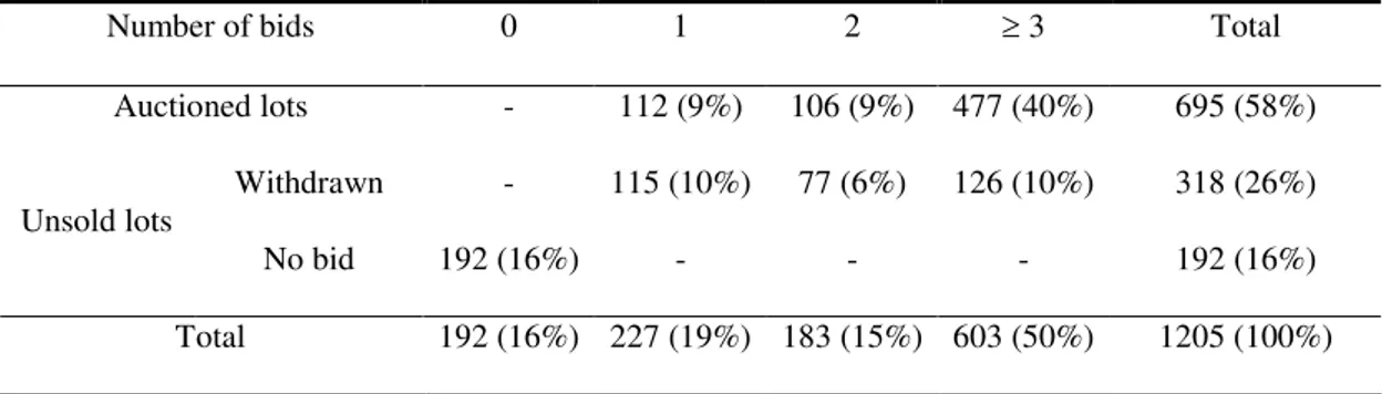
Lots may be classified according to the auction results. A lot sold during the auction is “auctioned”, whereas the others are “unsold lots”. The percentage of unsold lots is 42% and shows a relatively difficult wood market environment in Lorraine during that period. It is useful to distinguish between lots that got one or more bids but have nevertheless been withdrawn by the seller and lots that got no bid at all, referred to as the “no bid” category. Table 1 presents sale results according to the number of bidders.

[Insert Table 1]

In our empirical application, we first propose to distinguish timber lots which received no bid and lots for which we observe at least one bid. Second, among the submitted lots, we distinguish 3 categories depending on the level of competition:

i) there is no competition: 1 bid, ii) there is limited competition: 2 bids,

iii) there is strong competition: 3 bids or more.

The database includes more than one hundred variables that represent a large part of the information available in the catalogues. It also includes private information from ONF (harvesting conditions, quality of the lot, secret reserve price), data about the auction results (the number of bids, the auctioned prices) and computed data such as the Herfindahl index. This database is rich and exhaustive, it contains all the

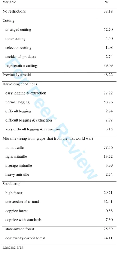
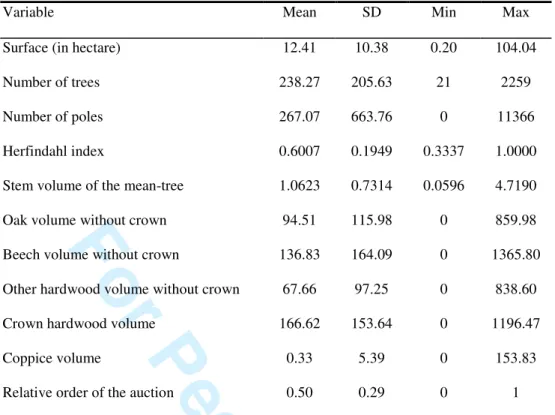
standing timber lots from public forests put on sale in the region during the fall of 2003. The following two tables give summary statistics of variables used in our econometric study. 3 4 5 6 7 8 9 10 11 12 13 14 15 16 17 18 19 20 21 22 23 24 25 26 27 28 29 30 31 32 33 34 35 36 37 38 39 40 41 42 43 44 45 46 47 48 49 50 51 52 53 54 55 56 57 58 59 60

For Peer Review

[Insert Table 2]

[Insert Table 3]

IV.

Methodology

Participation in timber auctions raises two econometric problems. First, many lots receive no bid and thus remain unsold. Secondly, the number of bidders has an impact on the result of the auction. Participation depends on the characteristics of the lots and thus is endogenous. We propose a reduced form econometric methodology that simultaneously deals with non-submitted lots (sample selection) and an

endogenous number of bidders in the hedonic price function. We explicitly model participation by constructing J categories; as announced, we consider 3 categories in our application: 1 bid, 2 bids, and 3 bids or more. We explain the intensity of

participation by the characteristics of the lots in an ordinal probit framework.

We propose a Bayesian MCMC sampling algorithm. Indeed the existing maximum likelihood estimation procedures (such as simulated maximum likelihood) do not perform well with multiple correlation coefficients and sample selection

(Waelbroeck, 2005). Thus, the idea is to simulate the (latent) variables that 3 4 5 6 7 8 9 10 11 12 13 14 15 16 17 18 19 20 21 22 23 24 25 26 27 28 29 30 31 32 33 34 35 36 37 38 39 40 41 42 43 44 45 46 47 48 49 50 51 52 53 54 55 56 57 58 59 60

For Peer Review

determine the participation outcomes, which greatly simplifies the analysis of the joint posterior distribution of the parameters.4

Despite the importance of the issue of sample selection with endogenous variables, we are not aware of a study that deals simultaneously with both issues. On the one hand, the problem of sample selection has been widely analyzed in the econometrics literature starting with the seminal work of Heckman, who proposed a method (Heckit) to correct sample selection bias. Van Hasselt (2005) has proposed a Bayesian MCMC algorithm to make inference on the correlation coefficient of the sample selection model. The author conducts a Monte Carlo study that shows that the Gibbs sampling algorithm performs well regardless of whether the parameters of the model are fully identified or not.5,6 _{On the other hand, Chakravarty and Li (2003)}

propose a Bayesian algorithm to test the effect of an endogenous binary variable on the profits of a trader (we are not aware of another similar study).

4 _{Indeed, latent variables can be simulated and, conditional on these variables, the model is a simple}

Seemingly Unrelated Regression (SUR) model that is easy to deal with. We use a Metropolis step to draw from the conditional posterior distribution of the elements of the covariance matrix of the unobservable variables.

5 _{The Gibbs algorithm is an MCMC algorithm that iteratively draws from the conditional posterior}

distributions of the parameters and always accepts such draws.

6 _{We propose a slightly different MCMC algorithm for the sample selection part of the model than}

Van Hasselt (2005). We write the latent model as a SUR model with an unequal number of observations; and thus inference on the coefficients of the observed equation only relies on observations that are not censored.

3 4 5 6 7 8 9 10 11 12 13 14 15 16 17 18 19 20 21 22 23 24 25 26 27 28 29 30 31 32 33 34 35 36 37 38 39 40 41 42 43 44 45 46 47 48 49 50 51 52 53 54 55 56 57 58 59 60

For Peer Review

We analyze endogenous participation in French public timber auctions using a system of three equations. Equation 1 determines the selection process: it is the probability that there is at least one bid. In case the bidders do not participate in the auction (no bid), the expected payoff of participating, w1,i, is zero or negative. Thus,

we define y1,i = 1 if at least one bidder participates in the auction and y1,i = 0

otherwise where i indexes the lots.

 1 if w1,i > 0

y1,i =  (1)

 0 if w1,i ≤ 0

where w1,i = x1,i′ β1 + ε1,i, β1 is of dimension k1 and x1,i is a set of control variables.

Equation 2 determines the outcome of the endogenous ordinal variable in the

selected sample. We define y2,i as an ordinal variable that can take on J values (in the

application J = 3).

 1 if w2,i ≤ α1

 ...

y2,i =  j if αj−1 < w2,i ≤ αj if y1,i = 1 (2)

 ...

 J if w2,i > αJ−1

where w2,i = x2,i′ β2 + ε2,i, β2 is of dimension k2 and x2,i is a set of control variables.

We define α = (α1, ..., αJ−1)′ as the vector of cutoff parameters to be estimated.

3 4 5 6 7 8 9 10 11 12 13 14 15 16 17 18 19 20 21 22 23 24 25 26 27 28 29 30 31 32 33 34 35 36 37 38 39 40 41 42 43 44 45 46 47 48 49 50 51 52 53 54 55 56 57 58 59 60

For Peer Review

Finally, Equation 3 is the hedonic price equation that explains the highest bid w3,i as

a function of lot characteristics and the endogenous ordinal participation variable y2,i

included as a set of J−1 binary variables.7 _{Equation 3 is only observed for lots that}

have received at least one bid (y1,i = 1).

w3,i = z3,i′ γ3 + z2,i′ δ2 + ε3,i = x3,i′ β3 + ε3,i observed for y1,i = 1 (3)

where z2,i = (z2,2,i, ... , z2,J,i)′ with z2,j,i = 1 if y2,i = j (and z2,j,i = 0 otherwise, j = 2, ...,

J), δ2 is a vector of parameters of dimension J−1, x3,i = (z3,i′, z2,i′)′ and β3 = (γ3′, δ2)′.

We assume that εi = (ε1,i′, ε2,i′, ε3,i′)′ is normally distributed with mean (0, 0, 0)′ and

covariance Σ for i = 1, …, n:

 1 ρ12 ρ13σ3 

Σ =  ρ12 1 ρ23σ3 

 ρ13σ3 ρ23σ3 σ32 

Parameters ρ12, ρ13 and ρ23 represent the correlations between the unobservable

variables. Hence, ρ13 is the correlation coefficient of the Heckman sample selection

procedure, while ρ23 is related to the lack of competition for the lot in the hedonic

7 _{We decompose the ordinal variable in a set of binary variables so that our results do not depend on}

the way we have coded the ordinal variable. This is not an issue in Equation 2 since the methodology automatically determine the cut-off points regardless of the values of the ordinal variable.

3 4 5 6 7 8 9 10 11 12 13 14 15 16 17 18 19 20 21 22 23 24 25 26 27 28 29 30 31 32 33 34 35 36 37 38 39 40 41 42 43 44 45 46 47 48 49 50 51 52 53 54 55 56 57 58 59 60

For Peer Review

price equation. Parameter σ32 is the variance of ε3,i. Since probit Equation 1 and

ordinal probit Equation 2 are not identified, we had to impose two restrictions. We chose to normalize the variances of the selection equation and of the endogenous binary variable to 1. These are standard restrictions in probit models.8

We always observe (x1,i, y1,i), but we only observe y2,i and w3,i when y1,i = 1.9

Moreover, the variables w1,i and w2,i are latent. The vector of explanatory variables

can be stacked in order to write the (partially) latent model as a SUR model with an unequal number of observations. Let n1 be the number of observations for which y1,i

= 0 and n2 the number of observations such that y1,i = 1, with n = n1+n2. We now

assume for notational convenience that the data have been sorted according to the values of y1. We also note the vector of binary dependent variables as y = (y1′, y2′)′.

Let β = (β1′, β2′, β3′)′, w1 = (w1,1, …, w1,n)′, w2 = (w2,1, …, w_2,n2)′ , w3 = (w3,1, …,

w_3,n2)′ and define w = (w1′, w2′, w3′)′. We define ε1, ε2, ε3 and ε in a similar fashion.

For notational convenience, we decompose the vectors of unobservable variables according to the selection process: ε = (ε11′, ε12′, ε2′, ε3′)′, where the second index

equals 1 if y1,i = 0 and equals 2 if y1,i = 1. Thus the covariance of the unobservable

variables is simply

8 _{See Wooldridge (2002) or any other textbook on the econometrics of qualitative dependant variable.} 9 _{The econometric model identifies all parameters associated with x}

1, x2 and x3 because of the

non-linearity of the Mill's ratio. However, in most sample selection specifications, some variables are usually not available for the censored observations, which means that the set of variables in x1 is

usually smaller than in x2 and x3.

3 4 5 6 7 8 9 10 11 12 13 14 15 16 17 18 19 20 21 22 23 24 25 26 27 28 29 30 31 32 33 34 35 36 37 38 39 40 41 42 43 44 45 46 47 48 49 50 51 52 53 54 55 56 57 58 59 60

For Peer Review

 I_n1 0 

Ω = Eεε′ =  0 Σ⊗I_n2 

where Ij denotes the identity matrix of dimension j×j. Thus Ω−1 is readily obtained.

We also decompose and stack the vector of the partially latent dependent variables as w = (w11′, w12′, w2′, w3′)′ and define similarly

 x11 0 0 

X =  x12 0 0  (n1+3n2)×(k1+k2+k3)

 0 x2 0 

 0 0 x3 

The (partially) latent model can be written in matrix format:

w = Xβ + ε (4)

Hence conditional on w and Ω, the estimates of β are simply obtained by a

Generalized Least Squares (GLS) regression of (4).10 _{Moreover, the matrices X′Ω}-1_X

and X′Ω−1w required for the GLS estimates of the parameters of the model are easily computed.

10 _{Since each stage contains different number of observations and generally different sets of}

explanatory variables, we can not estimate the SUR model with ordinary least squares regression applied to each latent equation separately.

3 4 5 6 7 8 9 10 11 12 13 14 15 16 17 18 19 20 21 22 23 24 25 26 27 28 29 30 31 32 33 34 35 36 37 38 39 40 41 42 43 44 45 46 47 48 49 50 51 52 53 54 55 56 57 58 59 60

For Peer Review

The 4 steps of the Metropolis-Gibbs algorithm and the computation of the partial effects are available upon request. We have used a flat prior in the Bayesian estimation of the parameters. The model can be extended to include informative prior so as to update implicit prices as the auction process moves on. However, with the large number observations that we have, this procedure is mostly relevant for the first auctions, given that at the end of the auction, the likelihood function will

completely dominate the prior distribution in the posterior distribution.11

V.

Results

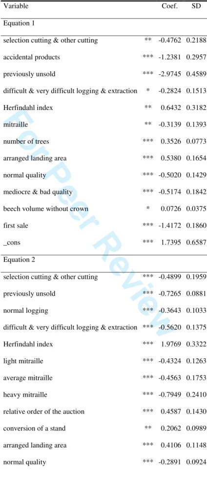
Table 4 gives the Bayesian estimation of the 3-equation model.12 _{All the variables}

available have been used to build the model but only significant variables have been kept in each equation. The signs of the estimated coefficients are coherent and intuitive, except for the variable ‘no restriction’ for which the coefficient is surprisingly negative in Equation 3.

11 _{To conclude this methodological section, one could wonder if we need three equations. Our model}

could have been written within an ordered probit framework if one only uses one latent variable for the number of bidders (lots without bids are interpreted as censored observations). However this specification is not as flexible, because it implies that the unobservable variable that determine whether a lot receives at least one bid is perfectly correlated with the unobservable variable that determine the number of bidders conditional on a lot receiving at least one bid. There are indeed good reasons to believe that these unobservable variables are not perfectly correlated.

12 _{Convergence of the MCMC algorithm was reach quickly. We removed the first 100000 iterations}

and kept the next 1000000 iterations for inference. 3 4 5 6 7 8 9 10 11 12 13 14 15 16 17 18 19 20 21 22 23 24 25 26 27 28 29 30 31 32 33 34 35 36 37 38 39 40 41 42 43 44 45 46 47 48 49 50 51 52 53 54 55 56 57 58 59 60

For Peer Review

Remember Equation 1 gives the probability that a lot will receive at least one bid. Equation 2 gives the intensity of competition (i.e the number of bidders). Equation 3 gives the estimated value of the log of the highest bid.

[Insert Table 4]

We also have estimated the probit Equation 1 and the ordinal probit Equation 2 separately and ran a Heckit procedure using sample selection Equation 1 and hedonic bid Equation 3 as benchmarks. Results were similar to the Bayesian estimation13_.

This is expected since the coefficient associated with the inverse Mills ratio is not significantly different from zero. However, this result is not reliable with the Heckit procedure and depends on the variables used to build the model. Actually, if we use only variables that are available in the sale catalogue, we may observe a selection bias while the Bayesian procedure does not detect any problem of sample selection bias.14 _{Therefore estimations of the correlation coefficients ρ}

13 using the Heckit

procedure can lead to misleading inference.

Controlling for endogenous participation and for the characteristics of the lots, we find that, compared to the highest bid for lots with two bids, on average: (i) lots with only one bid receive a highest bid that is 22.31% below and (ii) lots with three or more bids receive a highest bid that is 37.09% higher. These results on the cost of low competition are very significant and imply that it is important for the seller to have enough bidders for each timber lot. This objective must be kept in mind when

13 _{Results of these preliminary estimations are available upon request.} 14 _{Such a model is available upon request.}

3 4 5 6 7 8 9 10 11 12 13 14 15 16 17 18 19 20 21 22 23 24 25 26 27 28 29 30 31 32 33 34 35 36 37 38 39 40 41 42 43 44 45 46 47 48 49 50 51 52 53 54 55 56 57 58 59 60

For Peer Review

she determines the number of lots to put on the market, their size and their

composition. In addition, it would be wise to consider any improvement in the sale format that would lower the participation cost for any potential buyer.

Two other results deserve special mention. First, the degree of intra-lot heterogeneity is a significant variable in all 3 equations. Thus, competition increases for lots that are more homogenous in species, i.e. with an Herfindahl index closer to one. In addition, a higher Herfindahl index increases the highest bid. As shown by Boltz, Carter and Jacobson (2002) on prices of mixed species lots from timber auctions in North Carolina, increased heterogeneity leads to lower sale prices. In some way, they interpret such decrease in the revenue as an opportunity cost for ecosystem

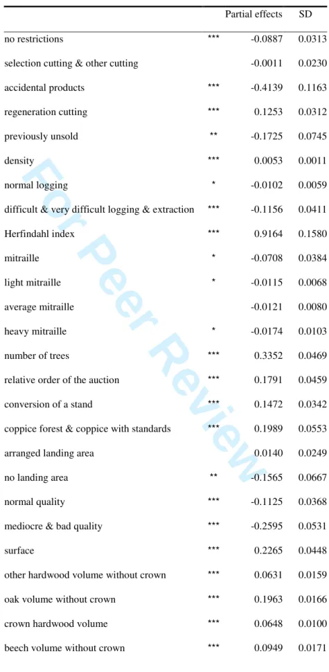
management where biodiversity is a desired constraint. Here, the opportunity cost of maintaining mixed forest can be estimated from the partial effect associated to the Herfindahl index: increasing the index by 1% increases the expected highest bid by 0.9164%. This figure can be found in Table 5 which gives the partial effect for every variable. The partial effect of a variable corresponds to the total impact of that variable on the expected log of the highest bid taking into account the possible selection bias of non submitted lots and the impact of that variable on the number of bidders.

Second, the coefficient associated with the ‘relative position of a lot’ in the sale is significantly positive in Equations 2 and 3. This indicates that lots put on the market at the end of a sale have a higher probability to receive more bids and to obtain a better highest bid than lots auctioned in the beginning of the sale. This last result implies that the decline in prices often observed in sequential auctions is not present 3 4 5 6 7 8 9 10 11 12 13 14 15 16 17 18 19 20 21 22 23 24 25 26 27 28 29 30 31 32 33 34 35 36 37 38 39 40 41 42 43 44 45 46 47 48 49 50 51 52 53 54 55 56 57 58 59 60

For Peer Review

in our sample of timber auctions. On the contrary, prices tend to increase for

hardwood lots during a sale. This could be due to cautious behavior of the bidders in the beginning and more aggressive bids at the end of the auction day. This

interpretation is confirmed by two additional results. First, the probability that a lot receives at least one bid is significantly lower in the first sale of the campaign. The variable ‘first sale’ has a significant negative impact in Equations 1 and 2: bidders wait and see. Second, the variable ‘last sale’ has a significant positive impact in the hedonic price Equation 3. This result reinforces the ‘relative position of a lot’ variable on a larger scale. Indeed, the highest bid increases during a sale (which is composed of many timber lots put on sale the same day), moreover the highest bids tend to be higher in the tenth sale (the one that took place the last day of the timber sale campaign).

[Insert Table 5]

VI.

Conclusion

Using detailed data on timber auctions, we have highlighted the importance of endogenous participation on auction results, focusing on lots that do not receive any bids and on the degree of competition when lots receive at least one bid. We have proposed a methodology to deal with both issues at the same time. The econometric method can easily be extended to deal with truncated or censored dependant

variables in the hedonic price equation, when the reserve price is announced. 3 4 5 6 7 8 9 10 11 12 13 14 15 16 17 18 19 20 21 22 23 24 25 26 27 28 29 30 31 32 33 34 35 36 37 38 39 40 41 42 43 44 45 46 47 48 49 50 51 52 53 54 55 56 57 58 59 60

For Peer Review

Our results can help public forest services to determine a relevant reserve price for each lot according to its characteristics. In addition, our hedonic price function for stumpage value gives interesting information about the implicit price of each lot characteristic for optimal lot composition. We have discussed the impact of the relative order of the lot in the sale and the impact of the intra-lot heterogeneity, but our results show that many variables have a significant impact on the participation process and on the highest bid including the type of cutting, the type of stand, the harvesting conditions, the volume and the composition of the lot. These results can help the forest public services to manage forest more efficiently so as to offer more attractive lots. Besides, our results highlight on the high cost of the low participation in French timber auctions and lead us to recommend any measure that would

increase the number of bidders. In particular, it would be wise to implement any idea that would lower participating cost.

Finally, our methodology can also be useful for bidders to define a bid that increases their probability of winning at a lower cost. Models can be elaborated according to which variables are available to the agent just before the auction.

3 4 5 6 7 8 9 10 11 12 13 14 15 16 17 18 19 20 21 22 23 24 25 26 27 28 29 30 31 32 33 34 35 36 37 38 39 40 41 42 43 44 45 46 47 48 49 50 51 52 53 54 55 56 57 58 59 60

For Peer Review

References

Boltz F., Carter D., Jacobson M, 2002, "Shadow pricing diversity in U.S. national forests", Journal of Forest Economics, 8, 185-197.

Brannman L.E., 1996, "Potential competition and possible collusion in Forest Service Timber auctions", Economic Inquiry, 34, 730-745.

Brannman L.E., Klein D., Weiss L.W., 1987, "The price effects of increased competition in auction markets", Review of Economics and Statistics, 69, 24-32. Buongiorno J., Young T., 1984, "Statistical appraisal of timber with an application to the Chequamegon National Forest", Northern Journal of Applied Forestry, 1, 72-76.

Carter D.R., Newman D.H., 1998, "The impact of Reserve Prices in Sealed Bid Federal Timber Sale Auctions", Forest Science, 44, 485-495.

Chakravarty S., Li K, 2003, "A Bayesian Analysis of Dual Trader Informativeness in Future Markets," Journal of Empirical Finance, 10, 355-371.

Costa S., Préget R., 2004, "Étude de l’adéquation de l’offre en bois de l’Office National des Forêts à la demande de ses acheteurs", final report for ONF, pp. 112 Hansen R., 1986, "Sealed-Bid versus Open Auctions: The Evidence", Economic Inquiry, 24, 125-42.

Huang F.M., Buongiorno J., 1986, "Market Value of Timber When Some

Offerings Are Not Sold: Implications for Appraisal and Demand Analysis", Forest Science, 32, 845-854. 3 4 5 6 7 8 9 10 11 12 13 14 15 16 17 18 19 20 21 22 23 24 25 26 27 28 29 30 31 32 33 34 35 36 37 38 39 40 41 42 43 44 45 46 47 48 49 50 51 52 53 54 55 56 57 58 59 60

For Peer Review

Jackson D.H., McQuillan A.G., 1979, "A technique for estimating timber value based on tree size, management variables, and market conditions", Forest Science, 25, 620-626.

Johnson R.N., 1979, "Oral Auction versus Sealed Bids: An Empirical Investigation", Natural Resources Journal, 19, 315-335.

McQuillan A.G., Johnson-True C., 1988, "Quantifying Marketplace

Characteristics for Use in Timber Stumpage Appraisal", Western Journal of Applied Forestry, 3, 66-69.

Niquidet K., van Kooten C.G., 2004, "Are log markets competitive? Empirical evidence and implications for Canada-U.S. trade in softwood lumber", working paper 2004-04, Resource and Environmental economics and Policy Analysis Research Group, Department of Economics, University of Victoria, British Columbia, pp. 34.

Poirier D.J., Tobias J.L., 2007, "Bayesian Econometrics", in Palgrave Handbook of Econometrics, vol. 1 Econometric Theory, Mills and Patterson (Eds.).

Prescott D.M., Puttock G.D., 1990, "Hedonic Price Functions for Multi-product Timber Sales in Southern Ontario", Canadian Journal of Agricultural Economics, 38, 333-344.

Puttock G.D., Prescott D.M., Meilke K.D., 1990, "Stumpage Prices in

Southwestern Ontario: A Hedonic Function Approach", Forest Science, 36, 1119-1132.

Sendak P.E., 1991, "Timber sale value as a function of sale characteristics and number of bidders", Res. Pap. NE-657. Radnor, PA: U.S. Department of Agriculture, Forest Service, Northeastern Forest Experiment Station, pp.7.

3 4 5 6 7 8 9 10 11 12 13 14 15 16 17 18 19 20 21 22 23 24 25 26 27 28 29 30 31 32 33 34 35 36 37 38 39 40 41 42 43 44 45 46 47 48 49 50 51 52 53 54 55 56 57 58 59 60

For Peer Review

Van Hasselt M., 2005, "Bayesian Sampling Algorithms for the Sample Selection and the Two-Part Models", Computing in Economics and Finance n°241, Society for Computational Economics.

Waelbroeck P., 2005, "Computational Issues in the Sequential Probit Model: A Monte Carlo Study," Computational Economics, 26, 141-161.

Wooldridge, J.M., 2002, Econometric analysis of cross section and panel data, MIT Press. 3 4 5 6 7 8 9 10 11 12 13 14 15 16 17 18 19 20 21 22 23 24 25 26 27 28 29 30 31 32 33 34 35 36 37 38 39 40 41 42 43 44 45 46 47 48 49 50 51 52 53 54 55 56 57 58 59 60

For Peer Review

Table 1. Timber auction results

Number of bids 0 1 2 ≥ 3 Total

Auctioned lots - 112 (9%) 106 (9%) 477 (40%) 695 (58%) Withdrawn - 115 (10%) 77 (6%) 126 (10%) 318 (26%) Unsold lots No bid 192 (16%) - - - 192 (16%) Total 192 (16%) 227 (19%) 183 (15%) 603 (50%) 1205 (100%) 3 4 5 6 7 8 9 10 11 12 13 14 15 16 17 18 19 20 21 22 23 24 25 26 27 28 29 30 31 32 33 34 35 36 37 38 39 40 41 42 43 44 45 46 47 48 49 50 51 52 53 54 55 56 57 58 59 60

For Peer Review

Table 2. Descriptive statistics for binary variables

Variable % No restrictions 37.18 Cutting arranged cutting 52.70 other cutting 4.40 selection cutting 1.08 accidental products 2.74 regeneration cutting 39.09 Previously unsold 48.22 Harvesting conditions

easy logging & extraction 27.22

normal logging 58.76

difficult logging 2.74

difficult logging & extraction 7.97 very difficult logging & extraction 3.15 Mitraille (scrap-iron, grape-shot from the first world war)

no mitraille 77.56 light mitraille 13.72 average mitraille 5.99 heavy mitraille 2.74 Stand, crop high forest 29.71 conversion of a stand 62.41 coppice forest 0.58

coppice with standards 7.30

state-owned forest 25.89 community-owned forest 74.11 Landing area 3 4 5 6 7 8 9 10 11 12 13 14 15 16 17 18 19 20 21 22 23 24 25 26 27 28 29 30 31 32 33 34 35 36 37 38 39 40 41 42 43 44 45 46 47 48 49 50 51 52 53 54 55 56 57 58 59 60

For Peer Review

unarranged 80.41 arranged 15.93 none 3.65 Quality very good 4.07 good 34.85 normal 45.64 mediocre 12.61 bad 2.66 3 4 5 6 7 8 9 10 11 12 13 14 15 16 17 18 19 20 21 22 23 24 25 26 27 28 29 30 31 32 33 34 35 36 37 38 39 40 41 42 43 44 45 46 47 48 49 50 51 52 53 54 55 56 57 58 59 60

For Peer Review

Table 3. Descriptive statistics for continuous variables

Variable Mean SD Min Max

Surface (in hectare) 12.41 10.38 0.20 104.04 Number of trees 238.27 205.63 21 2259 Number of poles 267.07 663.76 0 11366 Herfindahl index 0.6007 0.1949 0.3337 1.0000 Stem volume of the mean-tree 1.0623 0.7314 0.0596 4.7190 Oak volume without crown 94.51 115.98 0 859.98 Beech volume without crown 136.83 164.09 0 1365.80 Other hardwood volume without crown 67.66 97.25 0 838.60 Crown hardwood volume 166.62 153.64 0 1196.47

Coppice volume 0.33 5.39 0 153.83

Relative order of the auction 0.50 0.29 0 1 Variables are defined in logs except variables in percentage.

3 4 5 6 7 8 9 10 11 12 13 14 15 16 17 18 19 20 21 22 23 24 25 26 27 28 29 30 31 32 33 34 35 36 37 38 39 40 41 42 43 44 45 46 47 48 49 50 51 52 53 54 55 56 57 58 59 60

For Peer Review

Table 4 - Bayesian estimation of the 3-equation model

Variable Coef. SD

Equation 1

selection cutting & other cutting ** -0.4762 0.2188 accidental products *** -1.2381 0.2957 previously unsold *** -2.9745 0.4589 difficult & very difficult logging & extraction * -0.2824 0.1513 Herfindahl index ** 0.6432 0.3182

mitraille ** -0.3139 0.1393

number of trees *** 0.3526 0.0773 arranged landing area *** 0.5380 0.1654 normal quality *** -0.5020 0.1429 mediocre & bad quality *** -0.5174 0.1842 beech volume without crown * 0.0726 0.0375 first sale *** -1.4172 0.1860

_cons *** 1.7395 0.6587

Equation 2

selection cutting & other cutting *** -0.4899 0.1959 previously unsold *** -0.7265 0.0881 normal logging *** -0.3643 0.1033 difficult & very difficult logging & extraction *** -0.5620 0.1375 Herfindahl index *** 1.9769 0.3322 light mitraille *** -0.4324 0.1263 average mitraille *** -0.4563 0.1753 heavy mitraille *** -0.7949 0.2410 relative order of the auction *** 0.4587 0.1430 conversion of a stand ** 0.2062 0.0989 arranged landing area *** 0.4106 0.1148 normal quality *** -0.2891 0.0924 3 4 5 6 7 8 9 10 11 12 13 14 15 16 17 18 19 20 21 22 23 24 25 26 27 28 29 30 31 32 33 34 35 36 37 38 39 40 41 42 43 44 45 46 47 48 49 50 51 52 53 54 55 56 57 58 59 60

For Peer Review

mediocre & bad quality *** -0.6658 0.1340

surface *** -0.2640 0.0818

other hardwood volume without crown *** 0.1603 0.0367 oak volume without crown *** 0.2575 0.0363 beech volume without crown *** 0.2094 0.0330 first sale *** -0.5220 0.1811 α1 *** 1.4265 0.4095 α2 *** 2.0618 0.0437 Equation 3 no restrictions *** -0.0884 0.0308 accidental products *** -0.4538 0.1116 regeneration cutting *** 0.1258 0.0311 previously unsold *** -0.1049 0.0366 density *** 0.0053 0.0011

difficult & very difficult logging & extraction ** -0.0910 0.0384 Herfindahl index *** 0.9270 0.1412

mitraille ** -0.0763 0.0348

number of trees *** 0.3735 0.0374 relative order of the auction *** 0.1635 0.0461 conversion of a stand *** 0.1413 0.0350 coppice forest & coppice with standards *** 0.1978 0.0541 no landing area ** -0.1563 0.0682 normal quality *** -0.1159 0.0298 mediocre & bad quality *** -0.2261 0.0485

surface *** 0.2348 0.0438

other hardwood volume without crown *** 0.0581 0.0162 oak volume without crown *** 0.1885 0.0171 crown hardwood volume *** 0.0646 0.0099 beech volume without crown *** 0.0964 0.0145 stem volume of the mean-tree *** 0.4507 0.0269 3 4 5 6 7 8 9 10 11 12 13 14 15 16 17 18 19 20 21 22 23 24 25 26 27 28 29 30 31 32 33 34 35 36 37 38 39 40 41 42 43 44 45 46 47 48 49 50 51 52 53 54 55 56 57 58 59 60

For Peer Review

first sale * 0.1139 0.0589

last sale *** 0.1617 0.0355

y2 one bid *** -0.2231 0.0581

y2 three or more bids *** 0.3709 0.0657

_cons *** 3.4837 0.1526 ρ12 -0.0147 0.0581 ρ13 -0.0482 0.1296 ρ23 -0.0254 0.1242 σ3 *** 0.3837 0.0093 3 4 5 6 7 8 9 10 11 12 13 14 15 16 17 18 19 20 21 22 23 24 25 26 27 28 29 30 31 32 33 34 35 36 37 38 39 40 41 42 43 44 45 46 47 48 49 50 51 52 53 54 55 56 57 58 59 60

For Peer Review

Table 5 – Partial effects

Partial effects SD no restrictions *** -0.0887 0.0313 selection cutting & other cutting -0.0011 0.0230 accidental products *** -0.4139 0.1163 regeneration cutting *** 0.1253 0.0312 previously unsold ** -0.1725 0.0745

density *** 0.0053 0.0011

normal logging * -0.0102 0.0059

difficult & very difficult logging & extraction *** -0.1156 0.0411 Herfindahl index *** 0.9164 0.1580 mitraille * -0.0708 0.0384 light mitraille * -0.0115 0.0068 average mitraille -0.0121 0.0080 heavy mitraille * -0.0174 0.0103 number of trees *** 0.3352 0.0469 relative order of the auction *** 0.1791 0.0459 conversion of a stand *** 0.1472 0.0342 coppice forest & coppice with standards *** 0.1989 0.0553 arranged landing area 0.0140 0.0249 no landing area ** -0.1565 0.0667 normal quality *** -0.1125 0.0368 mediocre & bad quality *** -0.2595 0.0531

surface *** 0.2265 0.0448

other hardwood volume without crown *** 0.0631 0.0159 oak volume without crown *** 0.1963 0.0166 crown hardwood volume *** 0.0648 0.0100 beech volume without crown *** 0.0949 0.0171 3 4 5 6 7 8 9 10 11 12 13 14 15 16 17 18 19 20 21 22 23 24 25 26 27 28 29 30 31 32 33 34 35 36 37 38 39 40 41 42 43 44 45 46 47 48 49 50 51 52 53 54 55 56 57 58 59 60

For Peer Review

stem volume of the mean-tree *** 0.4516 0.0276

first sale 0.1168 0.0787 last sale *** 0.1618 0.0348 3 4 5 6 7 8 9 10 11 12 13 14 15 16 17 18 19 20 21 22 23 24 25 26 27 28 29 30 31 32 33 34 35 36 37 38 39 40 41 42 43 44 45 46 47 48 49 50 51 52 53 54 55 56 57 58 59 60