Perturbation of a radially oscillating single-bubble by a micron-sized object

HAL Id: hal-01619237

https://hal.archives-ouvertes.fr/hal-01619237

Submitted on 5 Sep 2018

HAL is a multi-disciplinary open access

archive for the deposit and dissemination of

sci-entific research documents, whether they are

pub-lished or not. The documents may come from

teaching and research institutions in France or

abroad, or from public or private research centers.

L’archive ouverte pluridisciplinaire HAL, est

destinée au dépôt et à la diffusion de documents

scientifiques de niveau recherche, publiés ou non,

émanant des établissements d’enseignement et de

recherche français ou étrangers, des laboratoires

publics ou privés.

Perturbation of a radially oscillating single-bubble by a

micron-sized object

William Montes Quiroz, Fabien Baillon, Olivier Louisnard, B. Boyer, Fabienne

Espitalier

To cite this version:

William Montes Quiroz, Fabien Baillon, Olivier Louisnard, B. Boyer, Fabienne Espitalier.

Pertur-bation of a radially oscillating single-bubble by a micron-sized object. Ultrasonics Sonochemistry,

Elsevier, 2017, 35 (A), pp.285-293. �10.1016/j.ultsonch.2016.10.004�. �hal-01619237�

Perturbation of a radially oscillating single-bubble

by a micron-sized object

W. Montes-Quiroz

a

_{, F. Baillon}

a

_{, O. Louisnard}

a,_⇑

_{, B. Boyer}

b

_{, F. Espitalier}

a

a_{Centre RAPSODEE, UMR CNRS 5302, Université de Toulouse, Ecole des Mines d’Albi, 81013 Albi Cedex 09, France} b_{Laboratoire de Génie Chimique, CNRS, 4, alle Emile Monso, CS 84234, 31432 Toulouse, France}

Keywords: Acoustic cavitation Single bubble Levitation cell SBSL Bubble stability

a b s t r a c t

A single bubble oscillating in a levitation cell is acoustically monitored by a piezo-ceramics microphone glued on the cell external wall. The correlation of the filtered signal recorded over distant cycles on one hand, and its harmonic content on the other hand, are shown to carry rich information on the bubble sta-bility and existence. For example, the harmonic content of the signal is shown to increase drastically once air is fully dissociated in the bubble, and the resulting pure argon bubble enters into the upper branch of the sonoluminescence regime. As a consequence, the bubble disappearance can be unambiguously detected by a net drop in the harmonic content. On the other hand, we perturb a stable sonoluminescing bubble by approaching a micron-sized fiber. The bubble remains unperturbed until the fiber tip is approached within a critical distance, below which the bubble becomes unstable and disappears. This distance can be easily measured by image treatment, and is shown to scale roughly with 3–4 times the bubble maximal radius. The bubble disappearance is well detected by the drop of the microphone harmonic content, but several thousands of periods after the bubble actually disappeared. The delay is attributed to the slow extinction of higher modes of the levitation cell, excited by the bubble oscillation. The acoustic detection method should however allow the early detection and imaging of non-predictable perturbations of the bubble by foreign micron-sized objects, such as crystals or droplets.

1. Introduction

A single bubble driven by a large sound field in a levitation cell undergoes nonlinear periodic radial oscillations, exhibiting at each cycle a large expansion phase followed by a collapse. The high energy density at collapse time produces short visible light-pulse, termed single-bubble sonoluminescence (SBSL) [1–3]. When air is used as the dissolved gas, above a threshold in the driving ampli-tude, the energy focusing during the collapse produces tempera-tures high enough for air dissociation to take place, so that only argon and water vapor remain inside the bubble[4–10].

The bubble levitation cell is a now classical experimental setup used to observe this phenomenon. It is made of an acoustical res-onator, spherical[11,12], cylindrical[1,13–15]or cubic[1,16,17], driven by piezoelectric ceramics in its breathing mode at a few tenth of kHz. The bubble is trapped at the pressure antinode in the cell center by the so-called primary Bjerknes force, which, for amplitudes moderate enough, counterbalances buoyancy and maintains the bubble stable against translational motion[18–21].

Observation of a stable spherical bubble also requires diffusional equilibrium, which is achieved by adequately degassing the water

[1,6], down to 10–40% of the saturation concentration in the case of air[8,22,23]. The bubble must also be stable against shape instabil-ities, which is ensured in a given amplitude range[22,24,25].

Levitation cells owe their popularity to the fact that the radial dynamics of the trapped bubble closely follows the theoretical pic-ture of a bubble driven by an isotropic sound field in an infinite liq-uid domain[22,26,27]. The latter can be reasonably modeled by a small set of ordinary differential equations, allowing an efficient scan of the parameter set[28–31]. This theory has been success-fully used to explore the details of the light-emission mechanism

[32].

Owing to the absence of translational motion and perfectly peri-odic oscillations of the single bubble, levitation cells also consti-tutes a useful tool to study other aspects of acoustic cavitation, beyond sonoluminescence. In particular, the behavior of a bubble perturbed by a neighboring micron-sized object is an important issue for cavitation applications such as emulsification (droplets), crystallization (solid particles) or biological applications (cells). The presence of such an object sufficiently close to the bubble is expected to break the isotropy of the acoustic field. The perturbation ⇑ Corresponding author.

thus imposed on the purely radial liquid motion results in an hydrodynamic interaction between the bubble and perturbing object. This perturbation might shift the bubble position, produce shape instabilities and possibly bubble disappearance. In particu-lar, an unexplored issue is the measure of the critical distance below which the bubble feels the presence of an object of compa-rable size.

On the other hand, a bubble oscillating in the stable SBSL regime is known to show a clear acoustic emission. The latter can be recorded by an hydrophone or a focused transducer located near the bubble[21,33]. An easier and non-invasive method con-sists in recording the output signal of a small piezo-ceramics glued on the side of the levitation cell[1,33]. Holzfuss and co-workers showed that an SBSL bubble had a perfectly periodic acoustic signature, constituted of a rich set of harmonics of the driving fre-quency[21]. It can be conjectured that this signature would be modified when a perturbing object approaches or appears suffi-ciently close to the bubble. Thus, real-time acoustic monitoring of the levitation experiment may allow to detect otherwise non-predictable events such as a cell or droplet passing near the bubble, or the growth of a crystal in its neighborhood. Using this informa-tion may for example allow to trigger a camera and image the event as soon as possible.

This paper examines the feasibility of such experiments. Section2 describes the main lines of the experimental setup. In Section 3, we detail the method of acoustic monitoring and the signal treatment used to diagnose the bubble oscillation regime. In Section4, we show how the single bubble can be perturbed in a controlled manner, by slowly approaching a micron-sized carbon fiber. The bubble response to this perturbation is examined and a critical object-bubble distance for bubble stability is tentatively defined. Finally, Section5 combines the results of the precedent sections, and examines whether acoustic monitoring allows to con-veniently detect the bubble disappearance in such perturbation experiments.

2. Experimental setup

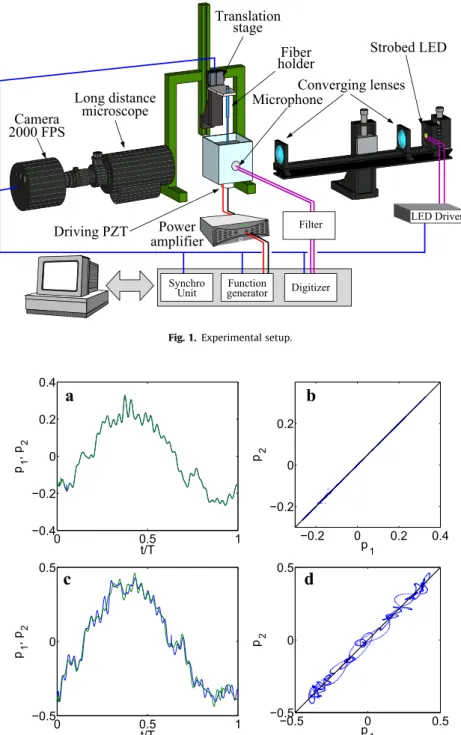
A resonator was made of a cubic optical glass cell (edge length 60 mm), filled with degassed water up to a level of 50 mm (Fig. 1). The cell is driven by a piezo-ceramic disc (PI Ceramics, PIC 155, 16 mm diameter, 5 mm thickness) glued at the bottom, and con-nected to a frequency generator through home-made impedance matching transformer and series compensation coil. The cell res-onates in its breathing mode at 21380 Hz. The acoustic emission of the bubble was recorded by a microphone made of a small piezo-ceramic disc (PI Ceramics, PIC 255, 10 mm diameter, 1 mm thickness), glued on the outer face of a lateral cell wall. The disc center is located at 25 mm above the cell bottom.

A second identical resonator was build after accidental breaking of the first one. Despite its design was rigorously identical to the latter, its resonance frequency was found to be 21,150 Hz. Finally, a spherical resonator was also used in some experiments. It was made of a spherical flask (60 mm inner diameter) driven by two laterally glued piezo-ceramics facing each other, the microphone ceramics being glued on the bottom. The resonance frequency of the spherical cell was 28,670 Hz.

The bubble is imaged by a fast camera (MIRO 310, 2000 FPS) through a long distance microscope (Questar QM 100) and light-ened by a white power LED (Luxeon Rebel LXML-PWC2). The wide-angle LED light emission is refocused at the microscope focus by two converging lenses, and the levitation cell is mounted on a three-axis stage so that the bubble can be positioned at the com-mon focus of the microscope and of the lightning system. Both the camera and the LED are synchronized externally by sending

pulses locked to a given phase of the frequency generator, so that when the bubble motion is periodic, its motion can be frozen to the required phase of its radial oscillation [16,17]. The LED flash duration could be as small as 500 ns.

The microphone signal was first amplified and filtered by a home-made analog 5th order Butterworth high-pass filter, of cut frequency 40 kHz. This allows to eliminate a large part of the driv-ing frequency without affectdriv-ing too much the first harmonics. The resulting signal is sampled by a 12 bit fast digitizer over exactly one acoustic period (2048 samples per period), at a constant phase of the driving. The unfiltered microphone signal and the voltage across the driving piezo-ceramics were also sampled in the same way. The function generator, digitizer and syncing unit all pertain to the same device (National Instruments PXI rack) and are con-trolled by the data-acquisition software LABVIEW.

Water was degassed in a closed stirred tank maintained at con-stant temperature. Air was removed with a vacuum pump, down to a controlled pressure. After one hour stirring, the tank was opened to atmospheric pressure and water was poured in the levitation cell by gravity. Because of the constraint imposed by the manipu-lation of the fiber (see Sections4 and 5), our levitation cells were necessarily open to the atmosphere, whereby the water unavoid-ably re-gas during the experiments. When needed, the dissolved gas content in the cell was therefore measured immediately before and immediately after the experiment with an oximeter (Hach-Lange HQ30d). The largest deviation found over a given experi-ment was 6% of the saturation concentration.

3. Acoustic monitoring of the bubble 3.1. Signal correlation

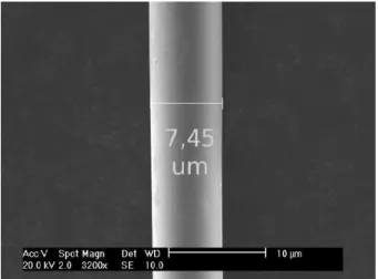
We first focus on the information that can be gathered on the bubble state by using the filtered signal recorded on the PZT micro-phone. A single recording event consists of two one-period records p₁ðtÞ and p2ðtÞ, separated by an integer number of acoustic periods

(1000 in the present case). When the bubble is stable, its motion is perfectly periodic and the two time series almost match exactly, as seen inFig. 2(a and b). Conversely, when the bubble motion is non-periodic, for example in the dancing regime, the two time series do not superpose (Fig. 2(c and d)).

The matching between the two time series can be quantified by calculating in real-time the correlation coefficient

C ¼ PM m¼1!p1;m$ p1"!p2;m$ p2" ffiffiffiffiffiffiffiffiffiffiffiffiffiffiffiffiffiffiffiffiffiffiffiffiffiffiffiffiffiffiffiffiffiffiffiffiffiffi PM m¼1!p1;m$ p1"2 q ffiffiffiffiffiffiffiffiffiffiffiffiffiffiffiffiffiffiffiffiffiffiffiffiffiffiffiffiffiffiffiffiffiffiffiffiffiffi_P M m¼1!p2;m$ p2"2 q ; _ð1Þ

where pi;m; i¼ 1; 2 denotes the mestpoint of the iestseries, piis the

mean of the latter, and M is the number of points in the series. A value of C close to 1 indicates a good periodicity of the voltage across the microphone and therefore a stable bubble.

In order to demonstrate the efficiency of this approach, we per-formed amplitude sweeps of the field driving the bubble. We start at a low amplitude and nucleate a bubble near the end of the dis-solving regime. Then, the generator amplitude was increased by small steps. Each level was maintained for 400 acoustic periods, allowing the bubble to reach steady state in the new conditions. Afterwards, the two time series p1ðtÞ and p2ðtÞ were recorded

and cross-correlated using Eq. (1). The whole process was then repeated at each amplitude step.

Operating this way, the bubble could be driven across all the well-known oscillation regimes of air single bubbles in degassed water[3,8,9,14,17].Fig. 3(top dotted curve, left ordinate scale) dis-plays the variations of C along one amplitude sweep for water degassed to 18% saturation, in function of the driving PZT voltage.

In the range labeled ‘‘A”, the bubble is in the dancing regime and the correlation parameter C of Eq.(1)takes random values smaller than 1. Above threshold ‘‘AD”, in the range labeled ‘‘B”, the non-noble gases in air N2 and O2 begin to react chemically. This

decreases the bubble ambient radius and restores sphericity and periodicity, so that parameter C becomes unity. Apart from a per-turbation labeled ‘‘PA” (see next section), the correlation parame-ter C remains close to unity over the whole ranges ‘‘B” and ‘‘C”, which shows that the bubble motion is periodic there. At the threshold voltage ‘‘SI”, the bubble disappears by shape instabilities. This causes a downward peak in C followed by a permanent drop of this quantity (hardly discernible onFig. 3).

3.2. Harmonic content

We also performed a real-time FFT of the filtered microphone signal over exactly one acoustic period.Fig. 4displays a waterfall plot of the 15 first harmonics magnitude in function of the driving field, for the same experiment as inFig. 3. It can be seen that sev-eral peaks, between harmonic 5 and harmonic 11, evolve signifi-cantly as the bubble is driven within its spherical stability range (zones B and C inFig. 3).

The dominant harmonic was found to depend on the dissolved gas content and as an empirical rule, we found that the higher the dissolved gas, the smaller the dominant harmonic. In order to get

−0.2 0 0.2 0.4 −0.2 0 0.2 p₁ p 2 0 0.5 1 −0.4 −0.2 0 0.2 0.4 t/T p 1 , p 2

b

a

0 0.5 1 −0.5 0 0.5 t/T p 1 , p 2 −0.5 0 0.5 −0.5 0 0.5 p₁ p 2

d

c

Fig. 2. Successive one-period samples of the filtered microphone output, distant of 1000 acoustic periods. (a) and (b): stable bubble; (a): Time plots p1ðtÞ and p2ðtÞ; (b): Phase

plot p2¼ f ðp1Þ; (c) and (d): same as (a) and (b), respectively, for a bubble in the dancing regime. The bubble instability can be readily concluded in the phase-plot when the

points wander around the first bisector, as in Fig. (d).

Camera

2000 FPS

Strobed LED

Converging lenses

Microphone

Long distance

microscope

amplifier

Power

Driving PZT

Fiber

holder

Translation

stage

Function _Digitizer Filter Synchro generator Unit LED Driver

an universal quantity independent of the dominant peak, an aver-age harmonic content was calculated in real time and monitored during the sweeps:

H ¼ X 15 n¼3 H2 n !1=2 : _ð2Þ

The middle curve (red online) inFig. 3displays the latter quan-tity, while the bottom curve (green online) is the amplitude of the dominant harmonic (10 in this case). It can be checked first that both quantities fall abruptly when the bubble disappears (event labeled ‘‘SI”), which is a useful criterion to detect the bubble disap-pearance. Moreover H10and H also undergo an abrupt positive jump

within the spherical stability region, at the threshold labeled ‘‘PA”. 3.3. Transition to pure Argon bubble

The threshold ‘‘PA”, where various bubble characteristic quantities (bubble ambient radius R0, maximum radius Rmax,

bubble position) undergo a jump within the spherical stability region, has been reported in earlier works [17]. It was found to be related to the chemical dissociation of air in the bubble [34]. On the left of the transition, the bubble still contains air, whose partial dissociation exactly balances the net influx by rectified dif-fusion[8]. On the right of the transition, the bubble collapse has become hot enough to fully dissociate air, so that argon remains the only gas in the bubble, in diffusive equilibrium with argon dissolved in liquid. Images recorded around the PA transition confirmed that the bubble also abruptly changed its position. The correlation defect visible on Fig. 3 can be thus attributed to the change in the bubble ambient radius and position between the two successive measurements. Furthermore, in absence of optical SBSL detection system, we cannot ensure that the PA tran-sition also marks the frontier between non-emitting bubbles and emitting bubbles. However, with the naked-eye, SL was never observed in region B, whereas it was always found in the upper range of region C. This is consistent with the current explanation of SBSL by air-dissociation hypothesis [3,8,9,14,22]. Moreover, the increase of the harmonic content, similar to the one observed here, has already been reported to appear at the lower SBSL threshold

[21].

In addition, it can be noted onFig. 3that the harmonic content undergoes a first peak before the PA transition (labeled ‘‘X” on

Fig. 3), associated with a correlation defect. This can be attributed to a first transition from a bubble still containing air to a pure argon bubble, but which is too small to heat enough during col-lapse, and reverts to the initial air-containing bubble. This behavior is the precursor of the chemical oscillations reported by Thomas and co-workers [17]. They found that for sufficiently large dis-solved air contents, the transition between non-emitting and emit-ting bubbles extends over a narrow range of driving amplitudes, in which oscillations of various bubble characteristics occurred on a timescale of a few seconds. This feature can be successfully caught by theory with a reduced bubble dynamics model including the process diffusive and reactive processes undergone by N2, O2,

and Ar[34]. We could easily observe such oscillations on the quan-tity H in experiments performed in water with larger air-content (not shown here for conciseness). Simultaneous imaging of the bubble confirmed the slow periodic translation of the bubble and variation of Rmax, similar to the one reported in[17]. As for the peak

labeled ‘‘X” onFig. 3, it can be attributed to the hysteretic character of the transition described above for low enough dissolved gas con-tent ([17],Fig. 4. This result suggests the coexistence of two attrac-tors and bi-stability in a narrow range of driving pressures [34]. The event observed at X might therefore correspond to a spurious jump between these two attractors, triggered by some yet unknown imperfection in our cell. The X and PA events are thus of similar nature except that at PA, the only stable attractor remaining is the pure Argon bubble.

The results of this section confirm that a proper treatment of the external microphone signal can yield rich information on the bubble characteristics, including whether the bubble has com-pletely rectified argon or not, and therefore whether it can undergo SBSL or not. In the experiments described hereinafter, only a diag-nostic of the bubble presence is required. If only bubbles in the regime ‘‘C” are considered, which will always be the case in this paper, it is seen that the sole examination of the drop in the quan-tity H offers a more than sufficient criterion.

4. Bubble perturbation by a neighboring object 4.1. Experiment

We now turn to examine the bubble stability against perturba-tions induced by the presence of a neighboring body. The latter

0 0.2 0.4 0.6 0.8 1

PZT

C

45 50 55 60 650 5 10 15 20 25 30 35 40

H

10

, H (mV)

C

D

X

PA

SI

H

AD

A

B

H

₁₀

Fig. 3. Dotted solid curve, left scale (blue online): correlation number C between two samples of the filtered microphone signal separated by 1000 acoustic periods, in function of the driving PZT voltage. Lower solid curve, right scale (green online): RMS value of the dominant harmonic (here 10th) of the microphone signal. Upper solid curve, right scale (red online): averaged RMS value of the harmonics in the range 3–15 [see Eq.(2)]. Region A: Bubble dancing regime; B: Stable bubble increasingly dissociating N2and O2; C: Stable pure argon bubble (SBSL); D: No

bubble; AD: Threshold for Air Dissociation; PA: Threshold for Pure Argon bubble; SI: Bubble disappearance by Shape Instability. (For interpretation of the references to colour in this figure legend, the reader is referred to the web version of this article.)

45 50 55 60 65 3 4_{5 6} 7 8₉₁₀ 1112₁₃₁₄ 15 0 5 10 15 20 PZT (V) n H n (mV)

Fig. 4. Waterfall plot of the harmonics of the microphone signal during the amplitude sweep, for the same experiment as in Fig. 3. The evolution of the correlation number C in function of the driving amplitude is recalled in dotted line (blue online). (For interpretation of the references to colour in this figure legend, the reader is referred to the web version of this article.)

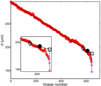
was made of a thin carbon fiber of about 7

l

m diameter (Fig. 5), glued on a syringe needle mounted on a manual x $ y and a motor-ized z-positioning system. The fiber was found to be rigid enough to be displaced almost vertically in the cell, without significant bending.

For each experiment, the following protocol was followed. A bubble was nucleated and driven in region C ofFig. 3. The bubbles considered hereinafter are therefore pure argon bubbles. The levi-tation cell was positioned so that the bubble was located at the bottom of the field of view and correctly focused. The phase of the LED stroboscope was adjusted to image the bubble at its max-imum radius. The fiber was pre-positioned by moving it along the optical axis x, and checking that its image was correctly focused by the microscope. Then, its y-position was adjusted so that along its expected vertical motion, the fiber tip would spear the bubble as close as possible to its centroid. Finally, the initial z-position of the fiber was set so that it just appears on the top of the field of view (see first image inFig. 6a).

The fiber was then displaced downwards by small steps, while the microphone signal was monitored, and the scene was imaged1_. Fig. 6(a) displays frames extracted from a typical sequence of the fiber motion. The last frame is the first image where the bubble is not anymore visible. It is seen that the bubble position remains stable over the major part of the fiber motion.Fig. 6(c) displays the last 10 frames before the bubble disappears, and shows that before doing so, the bubble slightly moves towards the fiber tip. 4.2. Critical stability distance dcrit

From the successive images of the bubble and the fiber, their motion could be reconstructed by straightforward image treat-ment.Fig. 6(b) displays the motion of the bubble centroid (solid line, red online) and of the fiber tip (dashed line, blue online) over the 643 last frames where the bubble is visible. The initial and final bubble locations are materialized by dashed and solid circles, respectively. The bubble translational stability during the major part of the fiber motion and its ultimate translation towards the fiber tip can be clearly seen on the centroid motion.

From these data, the distance between the bubble centroid and the fiber tip can be measured. The result is shown inFig. 7(round symbols, referred as ‘‘distance curve” hereinafter). The leftmost part of the curve is linear, because the fiber is moved at constant velocity, and the bubble centroid is initially stable. Below some threshold distance, the curve onFig. 7bends downwards, which suggest an increasingly marked motion of the bubble towards the fiber tip. The bubble disappears at the time materialized by the vertical dotted line.

The shape of the curve inFig. 7was found reproducible in all experiments, and suggests that the concept of a critical stability distance makes sense: above, the bubble centroid remains reason-ably stable, and below, the bubble markedly moves toward the fiber tip. Since the precise definition of the critical distance is somewhat arbitrary, the following method was used. First, the left-most part of the distance curve inFig. 7was fitted by a straight line. To do so as cleanly as possible, we performed successive linear fits of the distance curve starting from the two leftmost points, and adding each time a new point towards increasing times. The fit yielding the highest correlation was then drawn (Fig. 7, solid line) and the intersection of the latter with the vertical line issued from the last point was calculated (square symbol). This yields a first estimation of the critical distance. A second estimation is obtained by detecting the point from which the distance curve departs

forever from the fitting line by more than 1

l

m (diamond symbol). We defined the critical distance dcritas the mean between the two

ordinates (filled round symbol). A corresponding error bar was defined as the difference between the two estimations.

The result was found to be almost independent of the total number of points considered and of the criterion for calculating the second estimation, which suggests that the method is robust enough to extract reasonably well the critical distance from the data. We emphasize that the sought quantity dcrit is not the

dis-tance between the fiber tip and the ultimate position of the bubble, which is poorly reproducible from one experiment to the other, but the distance below which the bubbles starts to move towards the fiber. In some occasions, in the ultimate part of its motion towards the fiber tip, the bubble performed quick lateral excursions, wandering chaotically around the fiber before disappearing. The situation is exemplified in Fig. 8(a), where the first part of the bubble motion is depicted the same way as in the ‘‘normal” case ofFig. 6(b), and the following erratic path of the bubble centroid is drawn with triangle signs. The initial motion of the bubble cen-troid is seen to be similar to the one encountered in the normal case [compare solid line onFigs. 6(b) and 8(a)]. This is confirmed by the shape of the distance curve represented inFig. 8(b), whose left part (round symbols) is very similar to the one ofFig. 7. The only difference is the subsequent erratic motion [triangle symbols inFig. 8(a and b)], which can be easily distinguished from the first part of the motion, and can be therefore removed automatically in the numerical treatment. Doing so, the algorithm described above can still be used on the first part of the curve [circle symbols on

Fig. 8(b)] in order to extract the critical stability distance. We emphasize that the clear separation between the normal and erra-tic phases was found in all experiments where an erraerra-tic motion was observed, which allowed to cleanly rescue the latter ones. 4.3. Scaling of dcritwith maximum bubble radius.

Experiments were repeated for different bubbles driven in region C of Fig. 3, for various dissolved gas content ranging between 15% and 28% of air saturation, different driving pressures, and in the three levitation cells. Three different fibers were used, with the same shape, but unavoidably slanted with different angles with respect to the vertical. For each experiment, the critical stabil-ity distance was calculated as described in Section4.2. On the other hand, the maximum radius of the bubble Rmaxwas extracted from

the frames, and was found almost constant during the normal path of the bubble motion, except in a few cases. The Rmaxvalues were

averaged, and the deviations from the average allowed to define

Fig. 5. SEM photograph of the carbon fiber.

1 _{SeeSupplemental Materialat [URL will be inserted by publisher] to display a}

error bars for this quantity. For the experiments in the spherical cell, error bars on Rmaxwere estimated differently, because the

cur-vature of the flask yields an elliptic shape of the bubble image on the frames. Image treatment allowed to identify the two main axes of the ellipsis, from which a mean value and error bar on the bubble maximum radius were deduced.

Fig. 9displays the critical distance dcritin function of Rmaxfor the

whole set of experiments. Different symbols were used for the

three levitation cells, and filled symbols correspond to experiment where erratic motion was observed. Although no clear scaling law arises from this picture, it can be checked that the major part of the points cast between the lines dcrit¼ 3Rmax and dcrit¼ 4Rmax,

irre-spective of the acoustic pressure, the water gas content, and type of cell/frequency. This tendency suggests that correlating dcritwith

the bubble maximum radius Rmaxmakes sense.

We conjecture that the bubble disappearance is driven by the breakup of spherical symmetry as the fiber is approached. The presence of the fiber imposes a null liquid velocity in the vicinity of its tip, that is in a tiny region of space. This perturbation, despite being small, prevents the liquid to flow radially near the fiber, which favors bubble deformation if the tip comes close enough. Since the inward velocity attains huge values during collapse, the velocity constraint imposed by the fiber presence is expected to be more perceptible during collapse, and the bubble can be expected to break up during the latter. Moreover the collapse velocity increases with the mechanical energy stored by the bubble at its maximum radius[35], so that the perturbation caused by the fiber would be more intense for a more expanded bubble. A largely expanded bubble would thus be less stable against external pertur-bation. This is exactly the tendency demonstrated byFig. 9. The mechanism yielding the bubble breakup may therefore share some similarities with that producing asymmetric collapses near solid boundaries[36–38].

One may argue that the size of the perturbing object in the pre-sent case is much smaller than a plane boundary. However, it should be recalled that the problem of a bubble collapsing near an solid plane boundary is equivalent to that of two identical bub-bles in infinite fluid, symmetrically located on each side of a virtual plane replacing the solid boundary. The second bubble acts in this case as a mirror image of the first, ensuring a null velocity in the symmetry plane. As such, a bubble collapsing near an infinite rigid boundary can be in fact considered to interact with a mirroring bubble, which is an object of comparable size. Thus, despite the smallness of the fiber used in the present experiment, the latter

−100−50 0 50 100 −400 −300 −200 −100 0 100

b

c

a

Fig. 6. (a) Snapshots of the fiber and bubble positions as the fiber was moved downwards (frames between 1240 and 4140 by steps of 100). The last frame is taken just after the bubble disappearance; (b) Solid line (red online): motion of the bubble centroid reconstructed from image treatment on the last 643 frames before the bubble disappears; Dashed line (blue online): motion of the fiber tip. The initial and final positions of the bubble are materialized by a dashed circle and solid circle, respectively. The coordinates on axis are expressed inlm and the origin is chosen at the centroid of the final bubble position. (c) Last 10 frames before the bubble disappears. A slight motion of the bubble centroid towards the fiber tip is visible with the naked eye on the last but one frame. (For interpretation of the references to colour in this figure legend, the reader is referred to the web version of this article.)

0 200 400 600 150 200 250 Image number d (µ m) 600 150 200

Fig. 7. Open round symbols (red online): distance between fiber and bubble centroid, extracted from image treatment. Solid line (black online): linear fit on the leftmost N points yielding the highest correlation. Dashed line (blue online): vertical issued from the last point, which corresponds to the last frame where the bubble is visible. Square symbol: first estimation of the critical distance. Diamond symbol: second estimation of the critical distance. Filled circle symbol: final estimation of the critical distance. (For interpretation of the references to colour in this figure legend, the reader is referred to the web version of this article.)

somehow falls in the class of the well-studied collapse near a plane boundary (see[39], Chap. 10 and 11, and references therein for a review). In the latter problem, the bubble collapse becomes increasingly aspherical and undergoes jetting towards the solid wall as the dimensionless distance to the wall

c

¼ d=Rmax is

reduced. The critical distance measured here may therefore corre-spond to a critical asphericity of the collapse, above which the bub-ble cannot recover its initial form. In this respect, the sonoluminescence of laser induced bubbles was found to disappear for dimensionless distances

c

below about 3.5, because the col-lapse asphericity becomes too large[40]. The striking quantitative correspondence with the result ofFig. 9may be an indication that the bubble perturbation with the fiber investigated here is, in the end, closely related to the bubble behavior near a plane boundary. Moreover, two acoustically driven mirror bubbles attract together under the action of the secondary Bjerknes force[41,42]

as far as they do not come too close to each other[43,44]. One can thus conjecture that the ultimate accelerated motion of the bubble toward the fiber tip (see Fig. 6(c) and rightmost part of the curve in Fig. 7) can be interpreted in terms of a secondary

Bjerknes force between the bubble and some image bubble repre-senting the fiber.

In addition, it may be argued that the dispersion of the results onFig. 9is somewhat deceiving. However, it should be noted that manipulating such a thin fiber at this scale remains a difficult task. On one hand, as visible onFig. 6, the fiber could not be glued per-fectly vertically, in spite of our efforts. On the other hand, adjusting the respective initial positions of the bubble and the fiber was tricky, so that in some experiments, the fiber approaches the bub-ble slightly out of axis.

5. Acoustic detection of bubble perturbation

As evidenced in Section3, meaningful diagnostics can be made from the filtered microphone signal. In particular, the bubble dis-appearance is clearly accompanied by a drop in the harmonic quantity H. In this section, we examine to what extent the bubble disappearance caused by the fiber presence can be acoustically detected. More specifically, for practical applications, it is impor-tant to know the delay between the time at which the bubble suf-fers some perturbation and/or disappears, and the time at which the perturbation is actually detected by the microphone.

To investigate this issue, we performed experiments similar to the precedent ones, with the following differences. The drop of the harmonic quantity H was used to trigger the camera, which was set to the maximum FPS available (2000) during the fiber downward motion. The camera trigger was designed in such a way that the final movie retains 4414 ‘‘pre-trigger” frames, con-taining events that occurred prior to acoustic detection, and 200 ‘‘post-trigger” frames. In other words, the drop of H tells the camera to look back 4414 frames in the past (therefore covering a period of slightly more than 2 s). Looking at the past frames allows to see on which one the bubble really disappeared, and thus to measure the delay between its disappearance and its detection by the microphone.

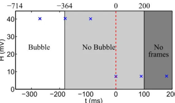
Fig. 10displays a typical result. The cross-signs indicate the amplitude of the microphone harmonic content H at the sampling times. The origin of time is set at the first microphone sample where a drop in H is observed. The trigger signal is sent to the

0 200 400 600 800 1000 1200 150 200 250 Image number d ( µm) −100 −50 0 50 100 −250 −200 −150 −100 −50 0 50 100 150

b

a

Fig. 8. Bubble undergoing erratic motion before disappearing (a) Motion of the bubble centroid. The first part of the motion is depicted as inFig. 6(b). The erratic part of the bubble path is displayed with triangle signs (pink online). The bubble radii at the first and final point of the erratic phase are materialized by gray (pink online) dashed circle and solid circle, respectively. (b) Distance curve. The erratic part of the motion is drawn with triangle symbols (pink online). (For interpretation of the references to colour in this figure legend, the reader is referred to the web version of this article.)

20 30 40 50 60 70 80 80 100 120 140 160 180 200 220 240 R_max (µm) d crit (µ m) dcrit = 4R max dcrit = 3R max

Fig. 9. Critical stability distance between the bubble centroid and the fiber, in function of the bubble maximum radius. Round symbols (red online): experiments in spherical cell (f = 28670 Hz); square symbols (blue online): experiments in first cubic cell (f = 21380 Hz); diamond symbols (pink online): experiments in second cubic cell (f = 21150 Hz). The filled symbols correspond to experiments in which erratic motion was observed. (For interpretation of the references to colour in this figure legend, the reader is referred to the web version of this article.)

camera at that time. The whole figure corresponds to 914 frames, 714 before trigger, and 200 after. The white region indicates frames where the bubble is present, and the light-gray shaded region frames with no bubble. From this figure, it is obvious that the bub-ble disappears about 180 ms before a perturbation is detected by the microphone, which corresponds to about 3800 acoustic cycles. This delay was found to be reproducible in all experiments.

Why the microphone is so late in detecting the bubble disap-pearance remains to be explained. The time for the perturbation to travel from the bubble location at the cell center up to the cell wall amounts to a=ð2cÞ where a ¼ 3:10$2_{m is the cell edge length}

and c = 1500 m/s is the sound velocity in water. This yields a delay of 20

l

s which far much smaller than the delay observed.

We suggest that this delay is rather due to a progressive extinc-tion of cell modes excited by the bubble. Indeed, when the bubble oscillates in the SBSL regime, its oscillations act as a periodic acoustic source with a well-defined harmonic content. For each frequency in the emission spectrum, a standing-wave mode builds up in the whole cell. Such standing waves were evidenced by Holz-fuss and co-workers (seeFig. 2in Ref.[21], displaying the mode of the 12th harmonics). The fact that the external microphone can hear these harmonics shows that the corresponding modes not only involve the liquid, but also the glass boundaries and the microphone itself. When the bubble disappears, these modes van-ish owing to various damping processes: viscous friction and ther-mal conduction in water, shearing in solid walls and in piezo-ceramics, Joule effect in piezo-ceramics. The smaller these damp-ing processes, the larger the extinction time. We conjecture there-fore that the delay is due to the ring-down time of the higher modes excited by the bubble oscillations, in a manner similar to a crystal glass which still rings a few seconds after having been hit. 6. Conclusions

A radially oscillating bubble in a levitation cell can be easily monitored by applying a simple treatment on the signal recorded by a small piezo-ceramic disk, glued on the external face of the glass wall. The bubble stability can be diagnosed by calculating the auto-correlation of this signal, whereas its harmonic content (above the third one) conveys a lot of information on the bubble regime. In particular, the amplitude of the total harmonic content allows to state whether the bubble oscillates in the chemical disso-ciation regime or in the SBSL regime. Bubble disappearance can also be detected unambiguously.

Bubble stability against the presence of a neighboring carbon fiber (7

l

m diameter) has been studied experimentally. Below a

critical distance between the fiber tip and the bubble, the latter moves towards the fiber and finally disappears. Provided the bub-ble was initially stabub-ble, the critical distance was found to cast roughly in the interval ½3Rmax;4Rmax&, irrespective of the type cell

used (spherical or cubic), the water gas content, and the acoustic pressure, and for frequencies ranging between 21,500 Hz and 28,500 Hz. As a rule of thumb, we therefore expect that a single levitating bubble will be disturbed by an object of a size compara-ble to its ambient radius if this object comes up to within 3 or 4 times its maximum radius. Further experimental and theoretical work is needed to examine the precise mechanism of bubble destruction by the fiber presence. It is conjectured that non-spherical collapses are involved, as they do for collapses near rigid boundary. The close agreement with the results of Ohl and co-workers[40], who found a critical stability distance of 3:5Rmax, is

rather striking, since the latter results where obtained with a laser bubble collapsing near an infinite solid boundary.

Finally, the bubble disappearance in such experiments can be easily correlated with an abrupt drop of the mean harmonic con-tent of the microphone signal. However the latter event was found to occur about 4000 acoustic cycles after the bubble actually disappeared. This delay may be attributed to the extinction time of the levitation cell modes excited by the bubble harmonics. For practical applications, these results demonstrates that despite acoustic monitoring is a simple and cheap method to detect non-predictable events occurring near the single bubble, it is thousands of acoustic cycles late in issuing the diagnostic. This phenomenon must be anticipated if one wish to use this method to get pre-trigger frames of a camera, for example by allowing for an oversized camera memory. Aside from this restriction, this opens the way to the easy detection of uncontrollable foreign objects, such as a micron-sized crystal, allowing its visualization as early as possible during its growth.

Acknowledgments

The authors acknowledges the support of the French Agence Nationale de la Recherche (ANR), under grant SONONUCLICE (ANR-09-BLAN-0040-02) ‘‘Ice nucleation control by ultrasounds for freezing and freeze-drying processes optimization”. The authors thank an anonymous referee for suggesting the compar-ison with the problem of the collapse near a plane boundary (espe-cially Ref. [40]), and another for motivating the discussion in

Appendix A.

Appendix A. Filtered microphone signal

The signals shown onFig. 1do not exhibit the typical pulse due to the shock wave emitted by the bubble oscillating in the SL regime (compare for example with Fig. 1a in Ref. [21] and

Figs. 1a and 2a in Ref.[33]). This is not our primary concern here since as shown in the text, the signal is rich enough to establish some useful diagnosis on the bubble. However, this issue is of gen-eral interest in the framework of single bubble experiments.

Several reasons may be responsible for the absence of this pulse. First, it must be recalled that our piezo-ceramic microphone is glued on the external face of the cell. It receives therefore the bubble emission (in particular the shock-wave pulse) through the vibrations of the cell glass walls. As mentioned in the last para-graph of Section5, a given frequency component of the pressure wave emitted by the bubble excites a standing wave in the liquid coupled to eigenmodes of the glass wall (probably flexural). The former were evidenced by Holzfuss and co-workers [21], who could measure standing waves corresponding up to the 56h

−300 −200 −100 0 100 200 0 10 20 30 40 t (ms) H (mV) −714 −364 0 200 No frames No Bubble Bubble

Fig. 10. Cross-signs: amplitude of H for each microphone sample. The origin of time corresponds to the trigger signal sent to the camera (dashed line). White region: frames where the bubble is visible. Light-gray region: frames where the bubble is not visible. Dark gray region: no frame. The frame numbers, relative to the trigger signal, are indicated above the figure. Negative numbers correspond to pre-trigger frames.

harmonic of the driving frequency in their levitation cell. Thus our microphone, which is not in contact with the liquid, can detect a given frequency only through the vibration of the corresponding flexural mode of the glass wall. The very short pulse width of 20 ns measured by Matula et al.[33]corresponds to a frequency of 50 MHz. The associated flexural modes would have very short wavelengths (which we can roughly estimate to 150 m at 50 MHz for a 2.5 mm-thick glass plate[45]). Such modes are likely to be strongly damped by visco-elastic dissipation since they involve high shearing. Moreover, the comparatively large area of the two piezo-ceramics glued on the wall (emitter and micro-phone) probably quench such short modes. In summary, we believe that the glass cell acts as a mechanical low-pass filter, and that there is no chance to observe the bubble emitted shock pulse on a microphone glued externally, contrarily to detec-tors immersed in the fluid (hydrophone or focused transducer

[33,21]).

The second reason for the absence of the shock pulse may be the bandwidth limitation of our home-made electronics. Low-cost operational amplifiers (Texas Instruments TL 082) were used in the pre-amplifier and filter connected to the microphone. The TL 082 is claimed to have a gain bandwidth of GBW = 4 MHz, so that transients of characteristic time as large as 1/GBW = 250 ns are already expected to escape our observation. The pulse originating from the bubble collapse reported by Matula and co-workers

[33]is one order of magnitude shorter (20 ns) and have thus no chance to be transmitted to the digitizer.

The first argument given above may also explain why the dom-inant harmonic in the spectrum of the microphone signal is not the second one, as is generally observed in multi-bubble fields[46]and confirmed by corresponding computations of the pressure wave emitted by the bubbles[47]. The coupled liquid/glass walls reso-nance modes excited by the single bubble emission probably have different resonant amplifications. This is confirmed by the spec-trum measured in Ref.[21](see their Fig. 1b and Table 1), which exhibits a local maximum of amplitude near the 7th harmonic and extends up to 4 MHz, with local maxima of comparable ampli-tudes visible up to 2.3 MHz. The second mode is probably quenched in levitation cells because the corresponding standing wave pattern is incompatible with the boundary conditions imposed, contrarily to multi-bubble configurations, where reso-nance effects with the vessel walls are probably masked by bub-ble–bubble interaction and random fluctuations of the bubble number[47].

Appendix B. Supplementary data

Supplementary data associated with this article can be found, in the online version, athttp://dx.doi.org/10.1016/j.ultsonch.2016.10. 004.

References

[1]D.F. Gaitan, L.A. Crum, C.C. Church, R.A. Roy, J. Acoust. Soc. Am. 91 (6) (1992) 3166–3183.

[2]S.J. Putterman, K.R. Weninger, Ann. Rev. Fluid Mech. 32 (2000) 445–476. [3]M.P. Brenner, S. Hilgenfeldt, D. Lohse, Rev. Mod. Phys. 74 (2) (2002) 425–483. [4]R.A. Hiller, R.K. Weninger, S.J. Putterman, B.P. Barber, Science 266 (1994) 248–

250.

[5]B.P. Barber, K.R. Weninger, S.J. Putterman, R. Löfstedt, Phys. Rev. Lett. 74 (1995) 5276–5279.

[6]R.G. Holt, D.F. Gaitan, Phys. Rev. Lett. 77 (1996) 3791–3794.

[7]D. Lohse, M.P. Brenner, T.F. Dupont, S. Hilgenfeldt, B. Johnston, Phys. Rev. Lett. 78 (7) (1997) 1359–1362.

[8]D. Lohse, S. Hilgenfeldt, J. Chem. Phys. 107 (17) (1997) 6986–6997. [9]T.J. Matula, L.A. Crum, Phys. Rev. Lett. 80 (4) (1998) 865–868. [10]B.D. Storey, A.J. Szeri, Phys. Rev. Lett. 88 (7) (2002) 074301-1–074301-3. [11]R.G. Holt, D.F. Gaitan, A.A. Atchley, J. Holzfuss, Phys. Rev. Lett. 72 (9) (1994)

1376.

[12]B. Gompf, R. Gunther, G. Nick, R. Pecha, W. Eisenmenger, Phys. Rev. Lett. 79 (1997) 1405–1408.

[13]B.P. Barber, R.A. Hiller, R. Löfstedt, S.J. Putterman, K.R. Weninger, Phys. Rep. 281 (1997) 65–143.

[14]D.F. Gaitan, R.G. Holt, Phys. Rev. E 59 (1999) 5495–5502. [15]J.A. Ketterling, R.E. Apfel, Phys. Rev. E 61 (4) (2000) 3832–3837.

[16]Y. Tian, J.A. Ketterling, R.E. Apfel, J. Acoust. Soc. Am. 100 (6) (1996) 3976–3978. [17]C.R. Thomas, R.A. Roy, R.G. Holt, Phys. Rev. E 70 (2004) 066301.

[18]I. Akhatov, R. Mettin, C.D. Ohl, U. Parlitz, W. Lauterborn, Phys. Rev. E 55 (3) (1997) 3747–3750.

[19]F.G. Blake, J. Acoust. Soc. Am. 21 (5) (1949) 551.

[20]T.J. Matula, Philos. Trans. R. Soc. London, Ser. A 357 (1999) 225–249. [21]J. Holzfuss, M. Rüggeberg, R.G. Holt, Phys. Rev. E 66 (046630) (2002) 1–4. [22]S. Hilgenfeldt, D. Lohse, M.P. Brenner, Phys. Fluids 8 (11) (1996) 2808–2826. [23]M.P. Brenner, S. Hilgenfeldt, D. Lohse, Nonlinear Physics of Complex Systems,

Springer, 1996, pp. 79–97.

[24]Y. Hao, A. Prosperetti, Phys. Fluids 11 (6) (1999) 1309–1317. [25]J. Holzfuss, Phys. Rev. E 77 (2008) 066309.

[26]R. Löfstedt, B.P. Barber, S.J. Putterman, Phys. Fluids A 5 (11) (1993) 2911–2928. [27]B.D. Storey, A. Szeri, Proc. R. Soc. London, Ser. A 456 (2000) 1685–1709. [28]K. Yasui, Phys. Rev. E 56 (1997) 6750–6760.

[29]R. Toegel, B. Gompf, R. Pecha, D. Lohse, Phys. Rev. Lett. 85 (15) (2000) 3165– 3168.

[30]B.D. Storey, A. Szeri, Proc. R. Soc. London, Ser. A 457 (2001) 1685–1700. [31]P. Koch, T. Kurz, U. Parlitz, W. Lauterborn, J. Acoust. Soc. Am. 130 (5) (2011)

3370–3378.

[32]S. Hilgenfeldt, S. Grossmann, D. Lohse, Phys. Fluids 11 (1999) 1318–1330. [33]T.J. Matula, I.M. Hallaj, R. Cleveland, L.A. Crum, W.C. Moss, R.A. Roy, J. Acoust.

Soc. Am. 103 (3) (1998) 1377–1382. [34]J. Holzfuss, Phys. Rev. E 78 (2008) 025303(R).

[35]S. Hilgenfeldt, M.P. Brenner, S. Grossman, D. Lohse, J. Fluid Mech. 365 (1998) 171–204.

[36]T.B. Benjamin, A.T. Ellis, Phil. Trans. R. Soc. Lond. A 260 (110) (1966) 221–240. [37]W. Lauterborn, H. Bolle, J. Fluid Mech. 72 (1975) 391–399.

[38]O. Lindau, W. Lauterborn, J. Fluid Mech. 479 (2003) 327–348. [39]W. Lauterborn, T. Kurz, Rep. Prog. Phys. 73 (10) (2010) 106501. [40]C.D. Ohl, O. Lindau, W. Lauterborn, Phys. Rev. Lett. 80 (1998) 393–396. [41]R. Mettin, I. Akhatov, U. Parlitz, C.D. Ohl, W. Lauterborn, Phys. Rev. E 56 (3)

(1997) 2924–2931.

[42]N.A. Pelekasis, J.A. Tsamopoulos, J. Fluid Mech. 254 (1993) 501–527. [43]A.A. Doinikov, S.T. Zavtrak, Phys. Fluids 7 (8) (1995) 1923–1930. [44]A.A. Doinikov, Phys. Rev. E 64 (2) (2001) 026301.

[45] A.W. Leissa, Vibration of plates, Tech. Rep. ADA307623, DTIC Document, Ohio State Univ Columbus, 1969.

[46]M. Ashokkumar, M. Hodnett, B. Zeqiri, F. Grieser, G.J. Price, J. Am. Chem. Soc. 129 (8) (2007) 2250–2258.

[47]K. Yasui, T. Tuziuti, J. Lee, T. Kozuka, A. Towata, Y. Iida, Ultrason. Sonochem. 17 (2) (2010) 460–472.