Analysis and application of two complementary numerical models for predicting flood waves generated by failures or dysfunctions occuring on a complex of dams

ANALYSIS AND APPLICATION OF TWO COMPLEMENTARY

NUMERICAL MODELS FOR PREDICTING FLOOD WAVES

GENERATED BY FAILURES OR DYSFUNCTIONS

OCCURING ON A COMPLEX OF DAMS

B.J. Dewals(1,2), S. Erpicum(1), P. Archambeau(1), S. Detrembleur(1) & M. Pirotton(1)

(1)

Research unit of Applied Hydrodynamics and Hydraulic Constructions (HACH), University of Liege, Chemin des Chevreuils 1 B52/3+1, 4000 Liege, Belgium,

Phone: +32 4 366 95 96; fax: +32 4 366 95 58; e-mail: B.Dewals@ulg.ac.be (2)

Postdoctoral Researcher of the Belgian National Fund for Scientific Research (FNRS)

ABSTRACT

A complete risk analysis related to a complex of dams may involve the assessment of a large number of different scenarios of failures and dysfunctions. However, a high computation time would be needed to perform a two-dimensional analysis of the flows generated by all possible scenarios. For this reason, the present paper expounds two complementary flow models, developed to be exploited within a rational methodology for analysing the flows induced by various incidents on a complex of dams and reservoirs.

The first model is the two-dimensional flow solver WOLF 2D, while the second one is a simplified lumped model, requiring very low computation time. An original analytical study is presented to demonstrate the conditions of applicability of the lumped model. This study leads to the practical conclusion that the evaluation of two non-dimensional parameters enables to assess a priori the validity of the simplified approach for any specific application.

The paper also describes the combined application of both models to a practical case study involving a complex of five dams. In a first step the lumped model has been validated by comparisons with the results provided by the two-dimensional model WOLF 2D. Secondly the simplified model has been successfully applied, at a very low CPU cost, to simulate flows induced by various dysfunctions and to conduct sensitivity analysis.

In conclusion, based on both theoretical developments and numerical studies, the paper provides new advances of practical relevance for dam break risk analysis.

Keywords: dam break, hydraulic modelling, risk analysis, complex of dams, dam breaching,

model, finite volume

1 INTRODUCTION

Flood waves induced by catastrophic events such as a dam break or a dam breaching are regularly studied, in the framework of risk analysis processes. However, other types of dysfunctions may also occur on a dam site (e.g. failure of penstocks, valves …) and are able to induce major damages in the downstream valley. Generally, those events are even characterized by a much higher probability of occurrence than the total collapse of the dam. Therefore studying the consequences of other system breakdowns is also necessary to properly perform a complete risk analysis on a hydraulic scheme.

Moreover, when such incidents take place on a complex of dams, additional specificities must be taken into consideration [13, 14]. In particular, the generated waves are likely to affect other dams of the complex and may breach them in cascade. As a consequence, risk analysis in such a case requires a holistic vision at the scale of the complex.

A prohibitive computation time would be needed to perform a complete two-dimensional analysis of the flows generated by all possible scenarios of dysfunctions on a complex. In contrast, an example of application of an efficient methodology appropriate for a complex of dams is illustrated in the present paper.

For this purpose, two complementary flow models are presented. The first one is the two-dimensional flow solver WOLF 2D, while the second one is a simplified lumped model, requiring very low computation time. They are intended to be combined optimally for predicting the flows induced by various incidents on a complex of dams and reservoirs

The paper details an original analytical study, which rigorously demonstrates the conditions of applicability of the lumped model. It can be concluded that two non-dimensional numbers must be evaluated to assess a priori the validity of the simplified approach for a specific application.

The paper also describes the validation and the application of the lumped model to a practical case study. In a first step the model has been extensively validated by comparisons with the results provided by the two-dimensional flow model WOLF 2D. Secondly the simplified model has been applied to a practical application involving a large gravity concrete dam located upstream of a complex of four other dams.

2 OVERVIEW OF THE MODELS

For more than ten years, the HACH research unit from the University of Liege has been developing mathematical and numerical tools for simulating a wide range of free surface flows and transport phenomena. Those various computational models are interconnected and integrated within one single software package named WOLF, which enables the simulation of process-oriented hydrology [10], 1D [10] and 2D hydrodynamics, sediment [3, 4] or pollutant transport [11], air entrainment [1], turbulence (incl. an original k-ε model [8]) … as well as an optimisation tool (based on Genetic Algorithms) [10]. Other functionalities of WOLF include the use of moment of momentum equations [2, 12], as well as computations considering vertical curvature effects by means of curvilinear coordinates in the vertical plane [2, 6].

Among those computation units, the two-dimensional flow model WOLF 2D will be more comprehensively described in the present paper. This model is able to represent flow regime changes (e.g. moving hydraulic jump), highly unsteady flows and shock waves.

It may also happen that dysfunctions on a complex of dams induce relatively gradual variations of the water level in the reservoirs, without inducing the propagation of stiff waves. In such a case, the computation cost can be drastically reduced by simulating the behaviour of the flow by means of a simplified flow model. Therefore, a lumped mathematical and numerical model is exploited to complement the two-dimensional model WOLF 2D. Moreover, this lumped model enables to undertake fast sensitivity analysis and to quickly compare flows generated by different scenarios of failures or dysfunctions.

3 DETAILED DESCRIPTION OF THE TWO-DIMENSIONAL FLOW MODEL

The two-dimensional model is based on the depth-averaged equations of volume conservation and of momentum conservation, namely the “shallow-water” equations. The large majority of flows occurring in rivers, even highly transient ones such as those induced by dam breaks, can reasonably be seen as shallow everywhere, except in the vicinity of singularities (wave tip).

The divergence form of the shallow-water equations includes the mass balance: 0 j j q h t x ∂ ∂ + = ∂ ∂ , (1)

and the momentum balance:

2 b f ; , 2 i j i ij i j i q q q h z g gh ghS i x y t x h δ x ⎡_{∂ ∂ ⎛ ⎞}⎤ _∂ + + + = − = ⎢_{∂ ∂} ⎜ ⎟⎥ _∂ ⎢ ⎝ ⎠⎥ ⎣ ⎦ , (2)

represents the bed elevation, h is the water depth, q designates the specific discharge in _i

direction i , S_fi is the friction slope and δ_ij the Kronecker symbol. The friction term is conventionally modelled thanks to an empirical law, such as Manning formula.

The space discretization of the 2D conservative shallow-water equations is performed by a finite volume method. Flux evaluation is based on an original flux-vector splitting technique developed for WOLF. The hydrodynamic fluxes are split and evaluated according to the requirements of a Von Neumann stability analysis [2].

WOLF 2D deals with multiblock structured grids. A grid adaptation technique restricts the simulation domain to the wet cell. Besides, the model incorporates an original method to handle covered and uncovered (wet and dry) cells. Thanks to an efficient iterative resolution of the continuity equation at each time step, a correct mass conservation is ensured [8].

Since the model is applied to transient flows, the time integration is performed by means of a second order accurate and hardly dissipative explicit Runge-Kutta algorithm.

WOLF 2D has been extensively validated by comparisons with experimental data, field measurements and other numerical models. Among others, benchmarks from EU Projects such as CADAM have been tested successfully. This validation process has been documented in previous papers [5-7, 9].

4 DETAILED DESCRIPTION OF THE LUMPED MODEL

An adequate simplified modelling approach for reproducing the behaviour of reservoirs consists in exploiting a lumped model, based on the volume balance only. Important simplifications are introduced in such a lumped model compared to the two-dimensional model. Indeed, since the free surface of the reservoir is assumed to remain almost horizontal, neither inertia effects, nor friction, nor the detail of topography are taken into account.

This approach does not involve an explicit description of the topography and the latter is simply depicted globally through the stage-capacity curve of the reservoirs. Possible inflow discharges must be provided, expressed as a function of time and/or of the water level. Outflow characteristics (e.g. control section with given crest level, crest width and discharge coefficient …) are also required as input of the model, while the outflow hydrograph itself is a computation result.

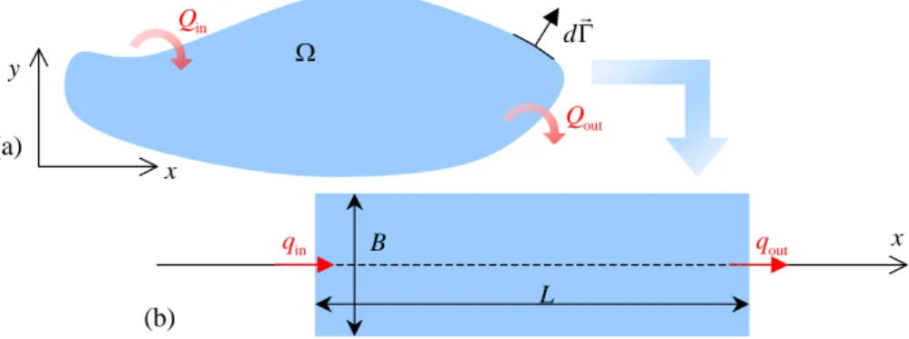
The two-dimensional model is based on the resolution of the depth-averaged equations of motion, expressing the conservation of volume and momentum along both directions x and y (see § 3). Integrated on the whole surface Ω (m²) of the reservoir i , equation (1) of _i conservation of volume becomes:

,in ,out 0 i i i i i dV h d q d Q Q t_{Ω Γ} dt ∂ _{Ω + ⋅ Γ = ⇔ = −} ∂

∫

∫

∑

∑

where Γ represents the contour of the reservoir, while _i V_i is the total volume, as sketched on Figure 1(a). Q_i,in and Q_i,out (m³/s) designate respectively the inflow and outflow discharges and N_R the number of reservoirs. The second formulation of equation (3), expressed in terms of stored volume and exchange discharges, constitutes the simplified lumped model for one reservoir. One equation of this type must be used for each reservoir of a complex. Of course, the formulation (3) of the model can also be written in terms of the water level Z_i (m) in the reservoir i , since the stage-capacity curve provides a relation between these two unknowns.

The set of equations (3) constitutes a system of NR ordinary differential equations, which are solved using an explicit time integration scheme. Such a numerical process requires the imposition of an initial condition relating to each unknown Vi (initial volume in each tank or,

x L B in q qout x y Ω dΓ in Q out Q

Figure 1: Sketch of a general reservoir and idealized 1D representation.

5 CONDITIONS OF APPLICABILITY OF THE LUMPED MODEL

This paragraph intends to provide a quantitative indicator, in the form of two non-dimensional numbers, enabling to judge a priori the validity of the approximation leading to the lumped model.

The main approximation implicitly introduced to derive the lumped model consists in disregarding equations (2) of momentum conservation. On the basis of a simplified theoretical approach, let’s check under which conditions this assumption may be considered as valid.

In order to focus on the most important aspects only, an idealized reservoir is considered, as illustrated by Figure 1(b). It is assumed to be straight and can be described by a characteristic length L (m), a characteristic width B (m) and a characteristic depth H (m). The effects of meandering and transverse distribution of the flow are thus neglected at this stage. As a consequence, the complete flow model (1)-(2) can be reduced to the following one-dimensional formulation, written per width unit:

0 h q t x ∂ ₊∂ ₌ ∂ ∂ (4) 2 s f z q q gh ghS t x h x ⎛ ⎞ ∂ ∂ ₊ ∂ _{+ =} ⎜ ⎟ ∂ ∂ _{⎝ ⎠} ∂ (5)

with z (m) the local free surface elevation, and _s S (m) the local friction slope. The latter _f

term will be neglected since it does not have a significant role in a reservoir.

In order to evaluate the order of magnitude of each term in equations (4)-(5), let’s define a characteristic variation of free surface elevation: Δ (m), a characteristic time T (s) and a zs characteristic discharge Q (m³/s). Since the continuity equation (4) is considered “as it”, without further simplification, to derive the lumped model, it is consistent to admit that both terms ∂ ∂h t and ∂ ∂q x are of the same order of magnitude. Consequently, the following relation between the characteristic values can be deduced:

( )

s

z T Q BL

Δ = . (6)

Besides, the lumped model relies implicitly on the assumption that the water surface remains quasi horizontal, and is thus characterized by a single value of Δ . To fulfil this condition, z_s

the only significant term in equation (5) of momentum conservation must be the gradient of the free surface, so that the equation reduces to: gh z∂ ∂ = . This is possible only if the _s x 0 first two terms of equation (5) are negligible, that means:

2 2 s s 1 1 , z z q Q B L T gh gH N t x T L gH ⎛ ⎞ ∂ Δ ∂ _{⇔ ⇔} ⎜ ⎟ ⎜ ⎟ ∂ ∂ _{⎝ ⎠} (7) (a) (b)

2 2 2 2 2 s s 2 1 , z z q Q B QT L T gh gH N x h x V L V gH ⎛ ⎞ ⎛ ⎞ ∂ Δ ∂ _{⇔ ⇔} ⎜ ⎟ ⎜ ⎟ _{⎜ ⎟} ∂ _{⎝ ⎠} ∂ _{⎝ ⎠} (8)

where relation (6) has been used, as well as the definition V =B H L.

Conditions (7) and (8) constitute quantitative criteria for assessing the validity of the lumped model. They take the form of two non-dimensional numbers which must remain low compared to unity. The first one, similar to a Froude number, expresses the need for the reservoir to be sufficiently small, so that perturbations propagate quickly enough everywhere. The second non-dimensional number expresses in addition that the total volume Q T , flowing in or out the reservoir, remains low compared to the capacity V .

6 CASE STUDY: DYSFUNCTIONS ON A COMPLEX OF FIVE DAMS

The two complementary hydrodynamic models have been applied to produce hazard maps downstream of a complex of large dams in the framework of a complete risk analysis.

6.1 Description of the complex of dams

The main dam (dam n°1), a 50 m-high concrete dam, is situated upstream of a complex of five dams, including a 20-meter high rockfill embankment one (dam n°2, located most downstream), and two main reservoirs. Figure 2 illustrates the global configuration of the complex of dams, which serves to enable navigation in the downstream waterways network during low-water periods and to produce hydroelectricity by pump-storage operations.

As a result of this layout of several dams, the hypothetical failure or other dysfunctions of the upstream dam (n°1) are likely to induce other dam breaks in cascade. Therefore the risk analysis of such a complex must be performed globally and not for each dam individually.

Prior to any hydraulic calculation, relevant scenarios of dysfunctions must be defined. The detailed analysis of the complex, which enables to identify those scenarios, lies beyond the scope of the present paper.

Upper reservoir Dam n°1: Concrete dam Lower reservoir Dam n°5 Dam n°2: Rockfill dam Dam n°4 Dam n°3 Downstream valley

However, this analysis leads to the conclusion that, focusing on the most upstream dam (n°1), the two main scenarios of major dysfunctions are [2]:

- scenario 1: the fracture of one or several of the four penstocks bringing water to the turbines of the power station situated at the toe of the dam,

- scenario 2: the total and instantaneous collapse of the dam.

As detailed below, in the case of scenario 1, the induced flow remains gradually transient (no significant effect of stiff waves propagation) and dam n°2 is assumed to be overtopped without breaching. In such conditions, the validity of the lumped model will be demonstrated (see § 7) and the model will provide the overflow hydrograph (downstream of the complex) without any calibration, since the crest of the submerged dam (n°2) remains a control section. A detailed sensitivity analysis will also be carried out at a very low computation cost (§ 8).

On the contrary, for scenario 2, dam n°2 would be severely overtopped and consequently breached, so that no control section remains and the 2D model becomes the most appropriate one. The lumped model would anyway remain a valuable tool to carry out sensitivity analysis of the released hydrograph with respect to the main breach parameters. Nevertheless, in this case, a specific calibration, based on the results of the 2D model, is needed to accurately compute the flow released through the breach, because of the influence of the flow downstream in the valley. This double approach clearly illustrates the complementarity of the lumped model and the two-dimensional one [2].

The present paper focuses on scenario n°1, for which the lumped model is applicable without calibration.

6.2 Formulation of the lumped model for the system of two reservoirs

The particular form of equations (3) for the two main reservoirs of the complex is expressed by the following system:

1 1,out dV Q dt = − (9) 2 2,in 2,out dV Q Q dt = − (10)

The inflow Q_2,in into the lower reservoir simply corresponds to the discharge Q_1,out

released from the upper one: Q2,in =Q1,out, while the discharge Q2,out released from the lower reservoir encompasses the water released through the spillway and by overtopping of dam n°2. As a consequence, those discharges are respectively expressed by:

(

)

1,out 2 1 2

Q =N A α g Z −Z , (11)

(

)

(

)

Spil. Spil. Spil. Crest Crest Crest

2,out 2 2 2 max 2 2 , 0 2 2 2 max 2 2 , 0

Q =b μ g_⎣⎡ Z −Z ⎤_⎦ +b μ g⎡_⎣ Z −Z ⎤_{⎦ , (12)}

where N designates the number of penstocks simultaneously undergoing a failure (N =1, 2, 3 or 4), A (m²) is the cross-section of one penstock (diameter: D=4.5 m), Z1 and

Z2 represent the water levels in, respectively, the upper and the lower reservoirs, and

(

)

1 2

1 k k

α −

= + + encompasses the local head loss coefficients at the entry (k1 = 0.5) and outlet (k2 = 1) of the penstocks. The continuous head losses have been verified to be negligible because of the short length. Spil.

2

b , Spil. 2

μ and Spil. 2

Z represent respectively the width, the discharge coefficient and the level of the spillway of dam n°2; while b₂Crest, μ₂Crest and

Crest 2

Z refer to the same characteristics for the whole crest of dam n°2.

7 VALIDATION OF THE LUMPED MODEL

upper reservoir, flows into the lower one and finally overtops dam n°2. This process is simulated by the lumped model and the results are compared to those generated by the two-dimensional model, which represents in details all the waves propagating in the reservoirs.

The lumped model is first validated for each reservoir separately. In each case either equation (9) or equation (10) is solved. After this stepwise validation, the model will be applied to compute the overflow hydrograph overtopping the downstream dam (n°2).

7.1 Step 1 – Emptying of the upper reservoir

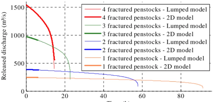
The first step of the validation is focused on the ability of the lumped model to predict the hydrograph characterizing the discharges released from the upper reservoir.

For the 2D simulation a Cartesian grid with cell sizes of 8 m is used. A zone of influence of the penstocks is defined, where the outflow discharge is extracted. The value of this discharge is updated at each time step according to equation (11), as a function of the current reservoir head Z1, while the level Z2 of the lower reservoir is temporarily assumed to remain constant. Head losses are temporarily neglected (α =1).

0 20 40 60 80 0 500 1000 1500 R e leased di schar g e ( m ³/ s) Time (h)

4 fractured penstocks - Lumped model 4 fractured penstocks - 2D model 3 fractured penstocks - Lumped model 3 fractured penstocks - 2D model 2 fractured penstocks - Lumped model 2 fractured penstocks - 2D model 1 fractured penstock - Lumped model 1 fractured penstock - 2D model

Figure 3: Hydrograph Q1,out of the flow released from the upper reservoir in case of a fracture of one to four penstocks of dam n°1, computed with the lumped model and the 2D model.

This 2D modelling reproduces reliably the waves dynamics in the reservoir, but requires a high computation time. Therefore, the 2D simulations are run only for a part of the total duration of the reservoir emptying, just sufficient to assess the consistency between the results of the two types of models. Indeed, the excellent adequacy between the results generated using the two models is showed by Figure 3. The differences never exceed 0.1 %, except in the final stage of the hydrograph, which is however not critical for risk assessment.

7.2 Step 2 – Inflow into the lower reservoir and overtopping of dam n°2

The second step of the validation is dedicated to verifying the ability of the lumped model to correctly predict the impact of the fracture of penstocks on the lower reservoir. First, a 2D simulation is again carried out to produce data of validation, which in turn is used as a reference to be compared with the results of the lumped model. The latter is applied by solving equation (10) expressing the volume balance for the lower reservoir.

Figure 4 represents the hydrograph entering the lower reservoir as a consequence of the simultaneous failure of four penstocks at dam n°1, as well as the computed hydrographs released through the spillway of dam n°2 and over its crest. The influence of the two terms of expression (12) is highlighted by the two successive rates of increase of the discharge, first flowing only through the spillway of dam n°2, then overtopping the crest as well.

The agreement between the predictions of the lumped model and the 2D one is satisfactory and corroborates the first step of validation. Moreover, the predicted maximum water levels are also in good adequacy. Thus it could be verified that the hazard map of

maximum water depth generated from the result of the lumped model fits remarkably well with the corresponding map issued by the 2D model [2].

0 2 4 6 8 10 12 14 16 0 500 1000 1500 Time (h) D isc h a rg e (m ³/ s) Inflow Q 2,in Outflow Q

2,out (lumped model) Outflow Q

2,out (2D model)

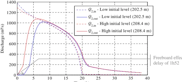
Figure 4: Hydrographs representing the inflow Q2,in into the lower reservoir and the discharge Q2,out released downstream of dam n°2, computed with the lumped model and the 2D model.

7.3 Discussion on the applicability of the lumped model

Two non-dimensional numbers were highlighted in § 5. Verifying that they remain low compared to unity provides a criterion for judging the expected adequacy between the results of a complete 2D model and those of the lumped model. Table 1 shows a comparison between the values taken by these non-dimensional numbers, both for the fracture of four penstocks (scenario 1) and for scenario 2. The characteristic length of the lower reservoir has been evaluated to 3500 m, while its characteristic depth is 18 M m³. Respecting the total capacity of the reservoir, the corresponding characteristic width is evaluated at 238 m.

Table 1 reveals that, for scenario 1, the non-dimensional numbers are both equal to approximately 0.02. In accordance with the theoretical development of § 5, this result corroborates the relevance of exploiting the lumped model in this case. On the contrary, the lumped model is confirmed to be inadequate for the study of the flow induced by the total collapse of dam n°1, since N1 and N2 take in this case values comparable to unity [2]. In conclusion, the theoretical analysis of § 5 is shown to be consistent with the results of the validation performed above as well as with the need already highlighted (§ 6.1) for a calibration if the lumped model is used as a tool to perform sensitivity analysis for scenario 2.

Table 1: Comparison of the non-dimensional numbers relevant for scenario 1 and scenario 2.

Dysfunction T (s) Q (m³/s) L / T (m/s) (gH)1/2 (m/s) N1 QT (m³) V (m³) N2 Scenario 1 300 3 104 12 13 0.88 9 10 6 15 106 0.69 Scenario 2 10800 1000 0,32 0.02 11 106 0.02

8 APPLICATION: SENSITIVITY ANALYSIS

After this stepwise successful validation, the lumped model is applied to perform a sensitivity analysis at very low CPU cost. From now on, the complete interaction between the levels of the two reservoirs is taken into consideration. Equations (9) and (10) are thus solved simultaneously, which will enhance the realism of the predicted hydrographs.

8.1 Influence of the initial level of the lower reservoir

The lumped model has first been exploited to evaluate the influence of the initial level in the lower reservoir and the benefits resulting from the freeboard height. The results produced on the basis of two different initial conditions are compared on Figure 5.

Release over the crest of dam n°2 Release through

the spillway of dam n°2

0 5 10 15 20 25 30 35 40 0 200 400 600 800 1000 1200 1400 Time (h) D isch a rg e (m ³/ s) Q

2,in - Low initial level (202.5 m)

Q

2,out - Low initial level (202.5 m)

Q

2,in - High initial level (208.4 m)

Q

2,out - High initial level (208.4 m)

Figure 5: Hydrographs representing the inflow Q2,in into the lower reservoir and the released discharge Q2,out downstream of dam n°2, for two different initial levels in the lower reservoir.

In a first time, the upper reservoir is supposed to be initially at a high level (208.4 m). This first assumption maximizes the total released volume but not the peak of the inflow hydrograph. The outflow hydrograph presents a peak value of 1073 m³/s. Secondly, the results obtained in the case of a low value of the initial level in the lower reservoir (202.5 m) is also shown on Figure 5. In this case, although the hydrograph released from the upper reservoir presents a higher peak value (1380 m³/s) than in the previous case (1293 m³/s), the peak value of the overflow on dam n°2 is damped as a result of the available freeboard and reaches a lower value (1019 m³/s) than previously. Moreover, this freeboard enables also an increase of almost two hours in the delay before the discharge is released into the downstream valley, which would facilitate operations of evacuation from the floodplains. The more critical assumption of an initially high level in the lower reservoir will be used from now on.

8.2 Influence of the number of simultaneously fractured penstocks

Secondly, the lumped model has been applied to efficiently compare the influence of the number of simultaneously fractured penstocks on the discharge released in the downstream valley. Figure 6 represents the time evolution of the discharges Q2,in and Q2,out as a function of the number of simultaneously fractured penstocks. The peak discharges released downstream of the complex in the case of one to three fractured penstocks correspond to respectively 27 %, 52 % and 77 % of the value released in the case of four fractured penstocks.

0 10 20 30 40 50 60 70 80 90 100 0 200 400 600 800 1000 1200 1400 Time (h) D isc h a rg e (m ³/ s)

Q_2,in - 1 fractured penstock

Q

2,out - 1 fractured penstock

Q_2,in - 2 fractured penstocks

Q_2,out - 2 fractured penstocks

Q_2,in - 3 fractured penstocks

Q

2,out - 3 fractured penstocks

Q_2,in - 4 fractured penstocks

Q_2,out - 4 fractured penstocks

Figure 6: Hydrographs representing the inflow Q2,in into the lower reservoir and the released discharge Q2,out downstream of dam n°2, as a function of the number of simultaneously fractured penstocks.

Freeboard effect: delay of 1h52

9 CONCLUSION

The paper depicts two complementary models to be used for efficiently computing the flows induced by various dysfunctions on a complex of dams. The first one is two-dimensional, while the second one is a lumped model requiring very low computation time. Besides, an original analytical analysis provides guidelines of practical interest for quantifying a priori the validity of the lumped model. Two non-dimensional numbers have been highlighted and can serve as efficient criteria for deciding whether the simplified model may be applied “as it”, namely without prior calibration. Comparisons are shown between the results of the 2D model and those of the lumped model in the case of a real application. They demonstrate the possibility of predicting the applicability of the lumped model on the basis of the two non-dimensional numbers mentioned before. Finally, the applicability of the lumped model is further illustrated through its exploitation for conducting economically a sensitivity analysis of the flow with respect to the scenarios of dysfunctions. This sensitivity analysis constitutes a key step in the process of risk analysis of a complex of dams, since it enables to identify the most relevant scenarios to be considered for computing the flood propagation in the downstream valley. In conclusion the paper outlines the benefits of combining a sophisticated 2D flow model and a simplified one, in the scope of simulating flood waves induced by dysfunctions on a complex of dams. It constitutes thus a bridge linking theoretical considerations with major concerns in the field of dam break risk analysis.

AKNOWLEDGMENTS

The authors gratefully acknowledge the Belgian Ministry of Facilities and Transport for funding the research project and for providing data.

REFERENCES

[1] André, S., et al., Quasi 2D-numerical model of aerated flow over stepped chutes, in Proc. 30th IAHR Congress, J. Ganoulis and P. Prinos, Editors. 2003, IAHR: Thessaloniki, Greece. p. 671-678.

[2] Dewals, B., Une approche unifiée pour la modélisation d'écoulements à surface libre, de leur effet érosif sur une structure et de leur interaction avec divers constituants. 2006, University of Liege: 636 p.

[3] Dewals, B., et al. Coupled computations of highly erosive flows with WOLF software. in Proc. 5th Int.

Conf. on Hydro-Science & -Engineering. 2002. Warsaw, Poland.

[4] Dewals, B., et al., Dam-break hazard mitigation with geomorphic flow computation, using WOLF 2D

hydrodynamic software, in Risk Analysis III, C.A. Brebbia, Editor. 2002, WIT Press. p. 59-68.

[5] Dewals, B.J., et al. Theoretical, numerical and experimental analysis of the hydrodynamic waves induced

by a dam break occurring on a complex of dams, and their impact on structures located downstream. in 7th National Congress on theoretical and applied Mechanics 2006. Mons, Belgium.

[6] Dewals, B.J., et al., Depth-integrated flow modelling taking into account bottom curvature. J. Hydraul. Res., 2006. 44(6): p. 785-795.

[7] Dewals, B.J., et al., Numerical tools for dam break risk assessment: validation and application to a large

complex of dams, in Improvements in reservoir construction, operation and maintenance, H. Hewlett,

Editor. 2006, Thomas Telford: London. p. 272-282

[8] Erpicum, S., Contribution à la modélisation de la turbulence en écoulements quasi-tridimensionnels à surface libre. Maillage adaptatif multibloc et calage objectif des paramètres. 2006, Univeristy of Liege.

[9] Erpicum, S., et al. Computation of the Malpasset dam break with a 2D conservative flow solver on a

multiblock structured grid. in Proc. 6th Int. Conf. of Hydroinformatics. 2004. Singapore.

[10] Erpicum, S., et al. Optimisation of hydroelectric power stations operations with WOLF package. in

Hydropower '05 - The backbone of sustainable energy supply. 2005. Stavanger, Norway.

[11] Erpicum, S., et al. Process-oriented pollutant transport modelling in rivers networks - Application in the

Xizhijiang River in China. in 3rd Int. Symp. on integrated water ressources management. 2006. Ruhr

University, Bochum, Germany.

[12] Khuat Duy, B., et al. Modelling suspended load with moment equations and linear concentration profiles. in 8th Int. Conf. on Fluvial Sedimentology. 2005. Delft, Netherlands.

[13] Marche, C., Barrages : crues de rupture et protection civile. 2004: Presses Internationales Polytechniques. 388 p.

[14] Marche, C., et al., Simulation of dam failures in multidike reservoirs arranged in cascade. J. Hydraul. Eng.-ASCE, 1997. 123(11): p. 950-961.