1
3D electrical resistivity tomography of karstified formations using cross-line
1measurements
2Van Hoorde Maurits, Dredging International NV, member of the DEME-group 3
Hermans Thomas, Stanford University, Geological Sciences, now at University of Liege, Urban 4
and Environmental Engineering, Belgium. 5
Dumont Gaël, University of Liege, Urban and Environmental Engineering, Belgium. 6
Nguyen Frédéric, Department of Civil Engineering, KU Leuven, Belgium 7
8
Corresponding author: 9
Hermans Thomas, [email protected] 10
The final version of this article is published in Engineering Geology, please cite as 11
Van Hoorde M., Hermans T., Dumont G., and Nguyen F. 2017. 3D Electrical resistivity 12
tomography of karstified limestone using cross-line measurements. Engineering Geology, 220, 13
123-132. http://dx.doi.org/10.1016/j.enggeo.2017.01.028 14
2 Highlights
16
1) We develop an innovative 3D ERT measurement procedure to image complex 3D resistivity 17
structure 18
2) The measurements procedure is based on the roll-along technique combined with cross-19
line measurements in several directions and distances 20
3) The procedure is optimized to minimize the required equipment and acquisition time on the 21
field 22
4) We show with synthetic and field measurements the increased imaging capacity of our 23
acquisition procedure compared to 2D parallel lines 24
Abstract 25
The acquisition of a full 3D survey on a large area of investigation is difficult, and from a 26
practitioner’s point of view, very costly. In high-resolution 3D surveys, the number of electrodes 27
increases rapidly and the total number of electrode combinations becomes very large. In this 28
paper, we propose an innovative 3D acquisition procedure based on the roll-along technique. It 29
makes use of 2D parallel lines with additional cross-line measurements. However, in order to 30
increase the number of directions represented in the data, we propose to use cross-line 31
measurements in several directions. Those cross-line measurements are based on dipole-dipole 32
configurations as commonly used in cross-borehole surveys. We illustrate the method by 33
investigating the subsurface geometry in a karstic environment for a future wind turbine project. 34
We first test our methodology with a numerical benchmark using a synthetic model. Then, we 35
validate it through a field case application to image the 3D geometry of karst features and the top 36
of unaltered bedrock in limestone formations. We analyze the importance of cross-line 37
measuring and analyze their capability for accurate subsurface imaging. The comparison with 38
3
standard parallel 2D surveys clearly highlighted the added value of the cross-lines measurements 39
to detect those structures. It provides crucial insight in subsurface geometry for the positioning of 40
the future wind turbine foundation. The developed method can provide a useful tool in the design 41
of 3D ERT survey to optimize the amount of information collected within a limited time frame. 42
Keywords: 3D electrical resistivity tomography, karstic environments, cross-line measurements, 43
electrode configuration 44
4 1. Introduction
45
In the last two decades, electrical resistivity tomography (ERT) has been widely applied in many 46
different contexts such as groundwater resources (e.g., Hermans et al., 2015; Yeh et al., 2015), 47
fault imaging (e.g., Nguyen et al., 2005; Suski et al., 2010) and geotechnical applications (e.g., 48
Chambers et al., 2013; Sauret et al., 2015). The wide range of applications of ERT is a result of 49
the large number of parameters influencing the electrical resistivity of the subsurface (porosity, 50
fractures, rock/soil type, saturation, temperature, fluid electrical conductivity, etc.) and the 51
robustness of the method. Because of the simplicity of field implementation, requiring only one 52
to two people for a couple of hours, 2D surveys are not time-consuming and relatively cost-53
effective. In addition, acquisition times have drastically decreased with the advent of multi-54
channel systems and automated switching systems (LaBrecque et al., 1996). Nevertheless, one of 55
the major drawbacks of 2D surveys is the underlying assumption that the subsurface is actually 56
2.5D, i.e. that electrical resistivity is constant in the direction perpendicular to the profile. This 57
assumption allows to successfully reduce the complexity of forward modeling from 3D to 2D 58
using a Fourier-cosine transformation (Dey and Morrison, 1979). Most interpretation software, 59
commercial or academic, uses this assumption in the inversion of 2D data sets. 60
The 2.5D assumption can be valid for certain conditions (profile perpendicular to main 61
geological structures, relatively homogeneous subsurface), but it can also lead to distorted and 62
misleading results in strongly variable and heterogeneous environments (e.g. Bentley and 63
Gharibi, 2004; Nimmer et al., 2008), such as encountered in karstic settings. In such cases or 64
when a detailed mapping of the subsurface is required, 3D acquisition and inversion techniques 65
must be considered. This remark is particularly true for karstic hazard where the 3D nature of the 66
5
dissolution processes makes the 2.5D hypothesis of the subsurface much weaker than for fault 67
imaging for example. 68
In most cases, the acquisition of a full 3D survey on a large area of investigation is difficult and, 69
from a practitioner’s point of view, very costly. The number of electrodes increases rapidly, the 70
time to acquire a complete data set and the required equipment are prohibitive. In most 71
applications, 3D surveys with a substantial number of electrodes (more than 100) are not full 3D 72
surveys but limited to the two main directions and the cross-diagonal (e.g., Li and Oldenburg, 73
1994; Kaufmann and Deceuster; 2007). Fiandaca et al. (2010) developed a 3D acquisition 74
procedure called maximum yield grid which limits the number of pairs of electrode used for 75
current injection and therefore reduce the impact on vulnerable surfaces such as archeological 76
sites (Capizzi et al., 2012). 77
However, to limit logistic constraints and optimize the acquisition time, 3D surveys are generally 78
designed as extensions of 2D surveys and can be performed with a limited amount of electrodes 79
connected to the resistivity meter at a certain moment in time. The most common solution is then 80
to deploy 2D parallel lines. The acquisition is 2D but the data are processed using a 3D inversion 81
code which accounts for heterogeneity in the direction perpendicular to the 2D lines (e.g., 82
Chambers et al., 2011; Orfanos and Apostolopoulos, 2011; Ustra et al., 2012). The extension in 83
both directions depends on the objectives of the investigation. Rücker et al. (2009b) used 12 long 84
lines of 140 electrodes with 3 m electrode spacing and 15 m line spacing, covering an area of 85
about 70 000 m2 to investigate a gold heap. In contrast, Papadopoulos (2010) carried out a square 86
survey of 26 lines of 26 electrodes with 1 m electrode- and line-spacing in tumuli investigations. 87
6
2D parallel surveys are relatively fast given the high number of electrodes generally used, but 88
they suffer from the limited 2D acquisition. Indeed the sensitivity to resistivity changes in the 89
perpendicular direction rapidly decreases for 2D surveys and most perpendicular structures 90
might be poorly imaged. To overcome this limitation, many authors have proposed to use 2D 91
lines in two orthogonal directions in order to acquire data in more than one direction (e.g., 92
Bentley and Gharibi, 2004; Berge and Drahor, 2011; Negri et al. 2008) Those studies have 93
shown that the inversion results of 2D orthogonal setups were more satisfactory, except if the 94
direction of the anomaly was already known or the electrode interspacing was sufficiently small. 95
For large domains, Rucker et al. (2009a) have shown that inverting the whole data set at once 96
yielded better results than inversions on sub-domains. 97
To consider data collection in more than two directions, some authors have also proposed radial 98
or star shaped surveys (e.g., Tsourlos et al., 2014; Nyquist and Roth, 2005), providing more 99
information on the heterogeneity of the subsurface in the central part of the investigated zone 100
Non-standard 3D surveys, such has C-shape or L-shape (e.g., Chavez et al., 2014), square-shape 101
(Argote-Espino et al., 2013) or ring-shape (Brunner et al., 1999) have also been tested in 102
complex environments where it is not possible to use electrodes on a large area. 103
However, both orthogonal and radial surveys ask for additional field work by increasing the 104
number of lines to acquire. Dahlin et al. (2002), in contrast, proposed a roll-along methodology 105
in the orthogonal directions to acquire simultaneously 2D parallel lines and orthogonal 106
measurements. It proposes to set-up several parallel lines at the same time and to acquire cross-107
line measurements in the orthogonal direction using electrodes already connected on the parallel 108
lines. When the first line has been acquired, it is removed and placed next to the last line as in 109
classical roll-along. Dahlin et al. (2002) tested the procedure with a pole-pole survey on a 17 110
7
lines survey with 21 electrodes, using 6 cross-line measurements (7 cables) in the orthogonal 111
direction only. This procedure reduces significantly the time spent on the field but provides a 112
data set less complete than a full orthogonal survey and still limits the number of measurement 113
directions during data acquisition. 114
In this paper, we propose an innovative 3D acquisition procedure based on the roll-along 115
technique of Dahlin et al. (2002). It makes use of 2D parallel lines with additional cross-line 116
measurements. However, in order to increase the number of directions represented in the data, 117
we propose to use cross-line measurements in several directions as proposed in Cho and Yeom 118
(2007) for imaging seepage in an embankment. Those cross-line measurements are based on 119
dipole-dipole configurations as commonly used in cross-borehole surveys. We illustrate the 120
method by investigating the subsurface geometry in a karstic environment for a future wind 121
turbine project. We first describe the field site and the geological context. Then, the designed 122
acquisition and processing procedure is described and assessed by numerical benchmark 123
modeling, using a synthetic model. We applied our validated methodology to the field case to 124
image the top of the unaltered limestone formation and to characterize the 3D geometry of karst 125
features. We then discuss the importance of cross-line measuring and analyze its capability and 126
optimal setup for correct subsurface geometry imaging. 127
2. Field site 128
The test site is located in the Couvin region, Belgium (Figure 1). It is a large area where a wind 129
turbine construction project is ongoing. As a preliminary study, a 2D electrical resistivity 130
tomography profile was performed by a private company (64 electrodes, 5 m spacing, NW-SE 131
direction) at the assumed location of each future wind turbine location. A large, medium 132
8
resistivity value anomaly (150-200 Ω.m) was detected beneath the location of one of the future 133
wind turbines. This anomaly was interpreted as an entity where limestone is heavily altered and 134
is supposedly linked to karstic phenomena present in the subsurface (see section 2.2). 135
Standard geotechnical investigations (such as cone penetration tests) would provide only 136
punctual information. Ideally, in such complex geo-hazardous environments, a 3D integrated site 137
investigation should be executed to construct a 3D subsurface geological model which can 138
support civil engineering and strategic design (e.g., Song et al., 2012; Ismail and Anderson, 139
2012). This concept was the motivation to conduct a 3D ERT survey at the location of the future 140
wind turbine. 141
2.1.Geology 142
The survey site region is located at the southwestern edge of the synclinorium of Dinant, a 143
geological structure composed of a succession of folded carbonate and terrigenous rocks (Marion 144
and Barchy, 1999b). The oldest lithostratigraphic unit in the study area is composed of the 145
formations of Saint-Joseph and of Eau Noire, consisting of layers of shale and thin limestone. 146
The second oldest formation is the formation of Couvin. It consists of very thick and compact 147
succession of limestone layers.. The youngest formation is the formation of Jemelle, mostly 148
consisting of shale layers (Marion and Barchy, 1999b). 149
9 150
151
Figure 1: Geological map of the site location. Red triangle represents the study area (modified
152
after Marion and Barchy, 1999a).
153
2.2. Karst characterization 154
10
Shallow karsts constitute a serious hazard to existing constructions and for civil engineering 155
projects due to the risk of resurgence, subsurface sinkhole development and subsidence (Sabbe, 156
2005; Samyn et al., 2014). The subsurface geometry thus needs to be very well characterized in a 157
systematic way when constructing in limestone settings (Alija et al., 2013). In the region of the 158
survey site, limestone can be locally highly fractured and karstified. Karst features are generally 159
filled with younger clayey sandstones and sediments (Marion and Barchy, 1999b) and can be 160
reactivated due to the present hydrogeological setting. 161
Karst features mostly develop in association with discontinuity planes (joints) by progressive 162
dissolution processes occurring under low hydraulic gradient. A soft weathering residue with 163
very high porosity (up to 50% or more), called ghost-rock or isalterite, may remain in place. In 164
areas of intense weathering, paleokarst features may interconnect leading to complex geometries 165
of weathered zones (Mihevc and Stepisnik, 2012). Through isalterite compaction, collapse and 166
transport, underground voids can open and migrate upward, forming sinkholes and typical karstic 167
topography (Kaufmann and Deceuster, 2014). 168
Ghost rock petrophysical properties show strong variations over short distances (Dubois et al., 169
2014). Kaufmann and Deceuster (2014) came to the conclusion that ghost-rock materials present 170
a lower density (down to 4 times less), higher porosity (up to 50 times more) and higher 171
permeability (up to 5 times more) than the surrounding limestone bedrock. 172
Due to the development of microporosity and suction phenomena, the weathering process in 173
isalterite results in a high saturation ratio, leading to a significant decrease in bulk electrical 174
resistivity. Geoelectrical methods are therefore among the most effective to detect and map 175
karstic structures (Dubois et al., 2015). Resistivity values lower than 50 Ω.m generally 176
11
correspond to silts and clayey sands at the surface and to highly weathered limestone at depth. 177
Resistivity values between 50 and 250 Ω.m correspond to dryer residual sediments/sandstones or 178
less weathered limestone at depth. Resistivity values larger than 250 Ω.m correspond to 179
competent bedrock. This rather low resistivity value is common for argillaceous limestones and 180
limestones with shale intercalation such those encountered in the study area (Ismail and 181
Anderson, 2012; Kaufmann and Deceuster, 2014). 182
Although no clear guidelines are prescribed for site investigations on karst landscapes, a 183
systematic approach should be developed to analyze karst environments to assess the risks, 184
establish guidelines for foundation design and avoid urban development in hazardous areas 185
(Pueyo Anchuela et al., 2015, Alija et al., 2013, Perrin et al., 2015). As suggested by Song et al. 186
(2012), ERT can be a valuable method to integrate in risk analysis for geo-hazards occurring in 187
karst regions. It can also serve as a tool for time lapse monitoring and continuous 188
characterization of karst features (Epting et al., 2009). 189
3. Methods 190
3.1. ERT survey design and protocol 191
The main objective of our survey design was to use the ABEM Terrameter LS (4 cables of 16 192
electrodes) equipment which is routinely used to execute 2D–ERT surveys. It was decided to use 193
a set of 18 parallel lines of 32 electrodes in combination with cross-line electrical resistivity 194
measuring, applying the 3D roll along technique to progress laterally through the designed 195
survey grid, connecting only 64 electrodes at a time. In-line measurements were performed along 196
each line, and cross-line measurements were performed in between parallel lines with a certain 197
offset with respect to a fixed chosen profile. The latter contain 3D resistivity information on the 198
12
subsoil in between parallel lines. The in-line electrode spacing is 5 m whereas the cross-line 199
electrode spacing is 10 m. 200
In-line measurements were acquired using a standard dipole-dipole configuration with a dipole 201
spacing a ≤ 20 m and a dipole separation n ≤ 6 times the dipole spacing, leading to a total 202
number of 436 measurements. The cross-line measuring concept is also based on a dipole-dipole 203
configuration (Figure 2). A dipole-dipole configuration has proven to be the most effective 204
electrode array in mapping complex subsurface geometry such as karst features (Zhou et al., 205
2000, 2002). The current and potential electrodes are located on two different lines. For all 206
current pairs, a maximum of 8 potential dipoles are considered, ensuring, cross-line 207
measurements at different angles to gather as much 3D information as possible within the setup 208
limits. The process is repeated for dipole spacing equal to 5, 10, 15 and 20 m, leading to a 209
number of measurements equal to 638 for each cross-line pair. 210
The inter-line spacing is increased and the process is repeated with the next line. In our survey, 211
cross-line measurements were taken at an offset of 20, 40 and 60 m. For large inter-line spacing 212
(40 and 60 m), a long interconnection cable was used to connect the cable to the terrameter unit. 213
13 214
Figure 2: Cross-line measurement concept. Red lines indicate the cables. Current and potential
215
electrode locations for two different injection dipoles are indicated with green and orange
216
crosses respectively.
217
The overall survey design can be reduced to a set of four unique profiles physically put in place 218
on the survey site (Figure 3). The survey as described here can be performed using 4 electrode 219
cables and a long interconnection cable. However, the use of 8 electrode cables reduces 220
significantly the amount of physical labor during field work. Note that it requires changing the 221
position of the Terrameter LS only 3 times. After data acquisition as depicted in Figure 3E, line 1 222
can be removed and installed as the next line of the grid (roll-along), while data are being 223
acquired as depicted by F, minimizing acquisition time on the field. Roll-along is routinely 224
applied until the final line is reached. Two different dipole-dipole protocols are used: one in-line 225
14
(applied to line L1 or line L2) and one cross-line between line 1 and 2 (C12). Figure 4 and Table 226
1 give a schematic overview of the survey plan. Table 1 also indicates which lines are active (C1, 227
C2, C3, etc.), where the ABEM Terrameter LS is positioned (A12, A45, A6, A7, etc.) and how 228
large the y-spacing is between the active lines (20, 40 or 60 m). The survey design is target and 229
location dependent, it can be altered to any alternative survey design based on different target 230
size, survey site requirements and constraints such as profile length and electrode spacing. 231
15 233
Figure 3: The developed survey design and plan of execution translated in profile line setup.
234 235
236
Position of ABEM + active cables
Y-spacing (m) Used protocol Situation in figure 2 A12_C1-C2 20 L1L2C12 A A12-C1-C3 40 C12 B A12-C2-C3 20 C12 C A45-C3-C4 20 L1L2C12 D A45-C1-C4 60 C12 E A45-C2-C4 40 C12 F A45-C2-C5 60 L2C12 G A45-C4-C5 20 C12 H A45-C3-C5 40 C12 I A6-C3-C6 60 L2C12 J A6-C5-C6 20 C12 K A6-C4-C6 40 C12 L A7-C4-C7 60 L2C12
16
A7-C6-C7 20 C12 From this point
onwards situation J, K and L are
routinely performed until
the end of the survey grid is reached. A7-C5-C7 40 C12 A8-C5-C8 60 L2C12 A8-C7-C8 20 C12 A8-C6-C8 40 C12 A9-C6-C9 60 L2C12 A9-C8-C9 20 C12 A9-C7-C9 40 C12 237
Table 1: Schematic overview of the survey script. In the left column the position of the ABEM
238
Terrameter LS is indicated by A followed by the line numbers in between which it is positioned.
239
The active cables are indicated by C followed by the line number.
240
17 242
Figure 4: Survey site geometry is depicted by a dark grey line. Blue lines indicate lines of survey
243
1, green lines indicate lines of survey 2. Together they form the combined survey lay-out. The
244
profile line ID number is indicated in red. The yellow dot is the location of the future wind
245
turbine.
18
The profile lines were oriented in a north-northeastern direction as perpendicularly to geological 247
structures as possible (Figure 4). Given that the minimum cross-line spacing is 10 m but the 248
minimum offset for crossline measurements is 20 m, it was chosen to split the total survey setup 249
in two surveys of nine profiles 155 m long (5 m electrode spacing).. The second survey line 250
setup has an offset of 10 meter with respect to the first survey setup (Figure 4), i.e. ‘in between’ 251
the profile lines of survey setup 1Survey 1 and 2 are depicted in Figure 4 by blue and green 252
profile lines respectively. The total grid length in the y-direction is 170 meter. The combined 253
survey grid consists of 576 electrodes, corresponding to a total number of 34644 measurements. 254
All electrodes were precisely positioned using a Trimble G8 GPS system. Note that due to 255
survey site geometry, the wind turbine’s location is not perfectly centered. 256
257
For acquisition, the delay time was set to 0.2 seconds and the acquisition time to 0.3 seconds. For 258
the same reason, we repeated the measurements maximum 3 times (2 if the error was below 1%). 259
We then used a limit of repeatability error of 1% to accept or reject a given measurement. 260
Injected current was fixed to 200 mA. 261
We deployed a team of 3 to 4 people on the field. Overall, it took 30-35 minutes to perform a 262
L1L2C12 measurement with the multi-channel ABEM Terrameter LS. For a C12 measurement 263
which measures only 1 crossline setup it took 12-15 minutes. Repositioning the resistivity meter 264
took 5 minutes. Moving a line in the y-direction took 10 minutes, but it can be performed while 265
measurements are running. Mobilizing and de-mobilizing the entire survey equipment spread 266
took 2 hours/day. 267
3.2. Data processing and inversion 268
19
Even though the use of dipole-dipole measurements with relatively large cross-line spacings 269
induced high geometrical factors, the average repeatability error on the apparent resistivity is 270
lower than 0.1%. However, to avoid our inversion to be affected by artifacts, the overall data set 271
(34644 points) was sorted to remove noisy data: 272
1) Measurements with low or zero current (bad electrode contact) are disregarded as they 273
correspond to injection failures (232 points) 274
2) Measurements with negative apparent resistivity are removed (2105 points) 275
3) To ensure sufficient signal to noise ratio, potentials below 0.1 mV were not considered 276
(149 points) 277
4) Points for which the repeatability error is above 1% are excluded (819 points) 278
The final data set considered for inversion thus contains 31339 measurements (90% of the full 279
dataset). 280
To assess the efficiency of cross-line measurements, different combinations of datasets were 281
created (Table 2). One of the data set corresponds to the individual in-line profiles. The other are 282
combinations of in-line and cross-line measurements from survey 1 or survey 1 and 2. The aim 283
of those subsets is to analyze which cross-line measurements are the most informative, in order 284
to reduce acquisition time in future 3D surveys. These 3D informative datasets were inverted 285
using RES3Dinv®. For all considered combinations, topography was included in the inversion 286
process. 287
All the inversions were carried out with the same inversion parameters. We use a L1 norm on the 288
data to reduce the effect of possible outliers and a L1 norm on the model (Loke et al., 2003) to 289
favor sharp contrasts of resistivity. 290
20
Despite, the low variance of the measured apparent resistivity, the final error of the inversion of 291
the full data set is still relatively high (more than 13%). In consequence, the data set was further 292
trimmed post-inversion based on the individual misfit of each simulated measurement versus the 293
observed one. We removed data points with a misfit greater than 20% (5300 data), allowing a 294
decrease of the RMS error to about 6% for the full data sets. For a fair comparison, other subsets 295
were built based on the sorted/trimmed full data set (Table 2). We stopped the inversions when 296
the RMS data misfit reached a value between 5 and 6%. 297
Survey 1 Combination of datasets
Number of data points in protocol number of data points after processing All IL + All CL 9 in-lines + 21 cross-lines 17322 12239 Survey 1+Survey 2
All IL 18 in-lines 7848 6721
All IL + CL 40 18 in-lines + 14 cross-lines 16780 12925 All IL + CL 60 18 in-lines + 12 cross-lines 15504 12264 All IL + All CL 18 in-lines + 42 cross-lines 34644 25469 298
Table 2: Different dataset combinations made for three dimensional inversion with RES3Dinv®.
299
ALL IL means all in line, ALL CL all cross-lines, CL # means that only the cross-line with #
300
spacing has been used.
301
3.3. DOI 302
We use the depth of investigation index (DOI) as an indicator of the depth below which the 303
model parameters are not constrained by the surface data anymore (Oldenburg and Li, 1999; 304
Oldenborger et al., 2007; Caterina et al., 2013). The DOI index can be calculated for every cell 305
by: 306
21
𝐷𝑂𝐼(𝑥, 𝑧) =𝑚𝑟𝑒𝑓1(𝑥, 𝑦, 𝑧) − 𝑚𝑟𝑒𝑓2(𝑥, 𝑦, 𝑧) 𝑚𝑟𝑒𝑓1− 𝑚𝑟𝑒𝑓2
with 𝑚𝑟𝑒𝑓1(𝑥, 𝑦, 𝑧) and 𝑚𝑟𝑒𝑓2(𝑥, 𝑦, 𝑧), the inverted model parameters obtained respectively with
307
mref1 and mref2 as reference models and (x,y,z) the coordinates of the cell. mref1 and mref2 have
308
a resistivity respectively ten times smaller and higher than the average apparent resistivity. The 309
relative weight given to the reference model during inversion is equal to 0.05. The DOI index is 310
generally used in its normalized form (DOInorm)by dividing the index vector by its maximum
311
value (DOImax) (Marescot et al. 2003):
312 DOInorm= DOI DOIMAX 313 𝐷𝑂𝐼(𝑥, 𝑧) =𝑚𝑟𝑒𝑓1(𝑥, 𝑧) − 𝑚𝑟𝑒𝑓2(𝑥, 𝑧) 𝑚𝑟𝑒𝑓1− 𝑚𝑟𝑒𝑓2
Indexes approaching zero mean that both inversions produce the same electrical structures and 315
therefore that the inverted model is still constrained by the data. Inversely, a DOI approaching 316
one means the model cells are less constrained by the data. A threshold value between 0.1–0.2 is 317
often chosen based on literature to calculate the depth of investigation (Oldenburg and Li, 1999; 318
Marescot et al., 2003; Miller and Routh, 2007). 319
4. Synthetic model 320
A numerical benchmark model is first carried out. the objective is to validate if our designed 321
survey method can image an artificially pre-defined 3D geological structure. 322
22 4.1. Description of the model
323
The synthetic model mimics the karstic environment expected at the study site. The numerical 324
geological structure consists of a central ridge of competent limestone with karstic features on 325
the sides (Figure 5). The different geological units are a sediment cover, 10 m thick (55 Ω.m), 326
weathered limestone with debris (450 Ω.m), ghost rock and tertiary sandstone filling karstic 327
features (250-300 Ω.m) and unaltered limestone bedrock (750 - 2500 Ω.m). RES3DMOD is used 328
to numerically simulate the apparent resistivity data corresponding to a pole-pole survey. Those 329
are subsequently used to build dipole-dipole dataset combinations similar to the one described in 330
section 3.2. We therefore use the detection of the shape and location of the central limestone 331
ridge as an indicator of the performance of the survey, since it is of uttermost importance for the 332
wind turbine project. This characteristic of the model will be highlighted by the 600 Ω.m iso-333
surface using the isoline methodology (e.g., Chambers et al., 2014b) and a horizontal slice. To 334
enhance the visualization of the ridge, the structures in the first 15 m below the surface are 335
disregarded. 336
4.2. Inversion results 337
The full data set is expected to bring the most valuable information on the 3D structure of the 338
model. As it appears in Figure 5, this data set allows to retrieve relatively accurately the location, 339
depth and shape of the ridge in the middle of the model. This observation confirms the survey 340
(in-line and cross-line spacing, number of parallel lines) was correctly designed. 341
23 343
. The models show a resistivity iso-surface of 600 Ω.m representing the transition to altered limestone 344
24
and a horizontal slice at 23 m depth. The model annotation corresponds to the dataset combination 345
overview provided in table 2. 346
All the reduced data sets retrieve less accurately the ridge structure. First, it appears that that the 347
use of a unique survey, i.e. an inter-line spacing of 20 m, is not able to image correctly the 348
subsurface. It detects the low resistive zone located at the origin of the grid and part of the ridge, 349
but not its complex 3D structure. Similarly, the use of the in-line data from both surveys is not 350
able to image correctly the 3D geometry, although general trends are detected. More specifically, 351
the absence of cross-line measurements impedes the detection of the transition to healthy 352
limestone. The good detection of the general trends lies in the orientation of 2D lines 353
perpendicular to the geological structures. Adding cross-line measurements to 2D lines clearly 354
improves the results. In this case, given the depth of the structure, cross-lines 40 m and 60 m are 355
the most informative. They enable us to refine imaging of the 3D structure. 356
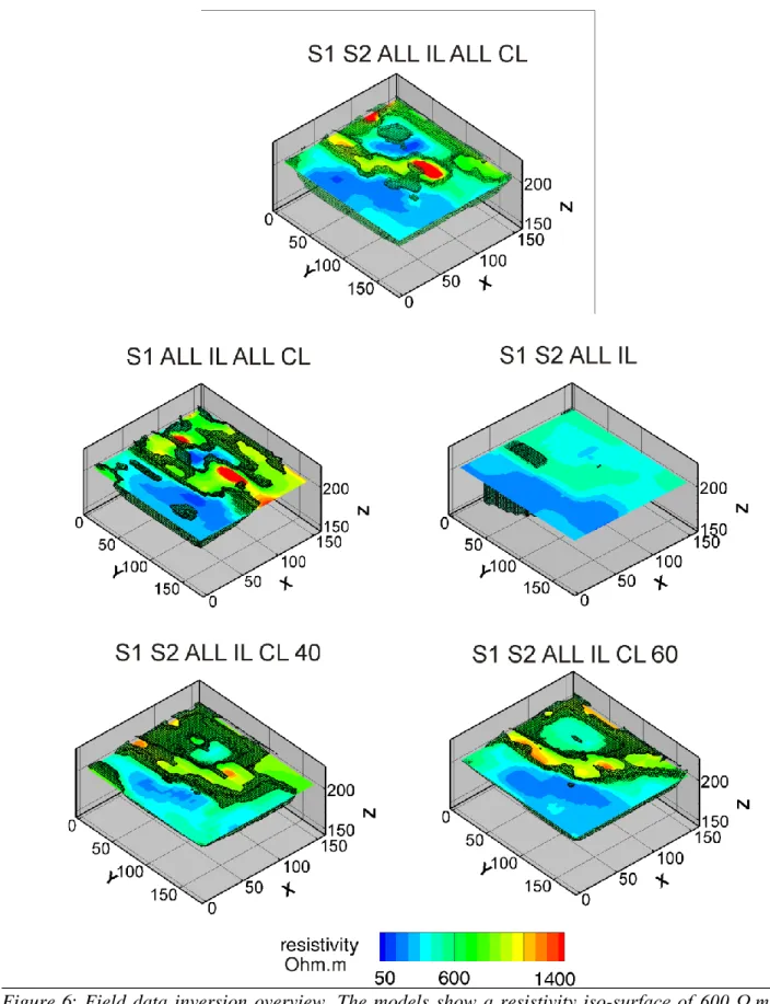
5. Field model 357
In the inversion of the full data set (Figure 6), a subsurface structure is recognizable with a 358
central ridge of unaltered limestone bedrock at a depth between 225 m TAW and 195 m TAW. 359
On its sides, two karstic features are clearly visible. The first is a large zone of low resistivity 360
value between X = 0 and X = 50 m, the healthy bedrock being detected at a depth of 195 m 361
TAW. The second is a smallest low resistivity zone located between Y = 50 m and Y = 100 m 362
and X = 75 m and X = 150 m. 363
25 365
Figure 6: Field data inversion overview. The models show a resistivity iso-surface of 600 Ω.m
366
representing the transition to altered limestone and a horizontal slice at the elevation of 205 m
26
(20 m depth). The model annotation corresponds to the dataset combination overview provided
368
in table 2.
369
The inversion of reduced data sets confirms the observation made for the synthetic case. Clearly, 370
the use of a spacing of 20 m between parallel lines is not sufficient to resolve the shape and 371
location of the limestone ridge. This subset of data incorrectly locates the ridge and its shape, and 372
adds undesirable high resistivity features in the area. The use of in-line data only qualitatively 373
detects most trends of the subsurface geometry with smaller resistivity contrasts, but the depth of 374
the unaltered bedrock is found deeper down (therefore not visible on the slice in Figure 6)Both 375
inversions with additional cross-line dipoles (40 m and 60 m) manage to image the subsurface 376
geometry as the full data set does. Those data sets image the second low resistivity anomaly with 377
a shape relatively similar to the reference. This observation is probably linked to the depth of the 378
targeted structures. Indeed, the cross-lines 20 m (not shown here), proved to be mainly helpful to 379
image 3D structure in the first meters below the surface (surface deposits). 380
As expected by the smaller data density at the beginning and ending of each survey line, the DOI 381
index remains small in the central part of the survey grid and increases towards the outer borders 382
(Figure 7). Using the dataset with a larger y-spacing (SI ALL IL ALL CL) induces high DOI 383
index values in the area where 3D geometry is most pronounced, reducing our confidence in the 384
detection of the ridge. The absence of cross-line data (SI S2 ALL IL) also induces a global 385
increase in the DOI index. The use of 40 m cross-line data is in this case the best alternative with 386
respect to the full data set. This dataset is able to capture 3D geometry at the required depth with 387
low DOI index values. Nevertheless, the absence of cross-line data at 20 m separation tends to 388
increase the DOI index at shallow depth. Using only cross-line data with a spacing of 60 m 389
induces a shortage of data in the data-set at shallow and medium depths where 3D structures are 390
27
present, increasing the DOI index. Those measurements are also characterized by higher 391
geometrical factors and therefore a less favorable signal to noise ratio. This may explain higher 392
DOI indexes observed in the zone corresponding to the first karstic anomaly. However, both 393
inversion clearly identified the contrast between the ridge and the karstic zone. Globally,it can be 394
stated that the central ridge structure observed in the inversions is constrained by the data. 395
For comparison, the 0.2 DOI limit of individual 2D sections (not shown) has an average depth of 396
12.5-15 meter in the central part of survey profile lines while it is around 42.5-45 meter for the 397
3D models. Cross-line data thus have a strong positive effect on the depth of investigation 398
28 400
Figure 7: 3D DOI index visualization. The horizontal slice of 200 m TAW is shown. A vertical
401
slice is depicted every 50 m.
29 403
6. Discussion and Conclusion 404
The most efficient way to conduct a three dimensional resistivity survey is to deploy a set of 405
parallel profile lines. However, the addition of measurements in other direction brings important 406
additional information on the 3D structure of the subsurface. In this paper, we propose an 407
innovative methodology to collect efficiently 3D electrical resistivity surveys. We combined the 408
standard 2D parallel acquisition with cross-line measurements, using the roll-along technique in 409
the perpendicular direction. In contrast to existing procedures, we include more than one 410
direction in cross-line measurements using dipole-dipole configurations similar to what can be 411
done in cross-borehole surveys. This procedure is a convenient and innovative way to execute a 412
3D informative ERT survey, using the same equipment as for a 2D ERT survey. 413
We applied this methodology on a synthetic case. It proves that such a data set is informative to 414
image the 3D resistivity structure of the subsurface. Especially, it is important to collect 3D 415
measurements with a depth of investigation coherent with the expected structure of the 416
subsurface. However, the collection of cross-line measurements must not be in detriment of a 417
sufficiently small spacing between parallel lines. The inter-line spacing should not be larger than 418
two times the in-line spacing to avoid unacceptable deterioration to the recovered resistivity 419
model. 420
The numerical results were validated by a field case study. We acquired on the field the proposed 421
3D in-line/cross-line surveys to image limestone formations subject to karstic features within the 422
context of a wind turbine project. Our methodology enabled us to successfully image the 423
presence of a central unaltered limestone ridge surrounded by much less competent rock affected 424
30
by karstic phenomena. The comparison with standard parallel 2D surveys clearly highlighted the 425
added value of the cross-lines measurements to detect those structures. The computation of the 426
depth of investigation index (DOI) has shown that the 3D DOI is 300% larger than the 2D DOI. 427
The cross-line data and 3D inversion have a positive effect on the depth of investigation to 428
constrain the 3D inverted model to greater depths. The produced 3D resistivity models provide a 429
thorough understanding of subsurface geometry, even for non-expert users. In the light of civil 430
engineering purposes, the visual power of these models will greatly help to improve 431
communication between geo-scientists and project engineers.The results provide crucial insight 432
in subsurface geometry for the positioning of a future wind turbine foundation, to the best of our 433
knowledge of the site. 434
In our case study, a 12-channel ABEM Terrameter LS resistivity meter was used. Time 435
optimized survey parameters greatly decrease survey time without drastically affecting data 436
quality. Indeed, in many cases, adding stacks will slightly decrease the repeatability errors and 437
increase the accuracy, but to a level not sufficient to accept the data for inversion. Using two 438
stacks and a cut-off of 1% in repeatability error appears to be a fast and efficient way to 439
accept/reject data points. 440
Trying to save survey time, and thereby reduce cost, by decreasing the amount of cross-line 441
measurements should be done only very carefully. The model quality decreases rapidly with 442
decreasing amount of 3D informative data. A survey setup, including in-line measurements and 443
cross-line measurements at 20, 40 and 60 meter should be respected. Using only cross-line data 444
is nevertheless a bad idea. Spatial coverage is not large enough within this survey setup; a basic 445
framework of in-line measurements should therefore always be acquired. If one would like to 446
reduce survey time and costs or if only four cables are available to perform the survey, the best 447
31
alternative is to use cross-line measurements at 40 m in this specific case. However, this 448
conclusion is likely dependent on the local geology and the targets of the survey. A thorough 449
pre-survey site study should be performed to adjust the survey design to the most suitable setup 450
for site specific conditions. 451
The mid-scale survey presented in this study took 2 days of survey preparation, 3 days of 452
fieldwork, and an extra week for data processing and reporting. In terms of cost, the 3D survey 453
was about 50% more expensive than a 2D survey of the same dimensions, but it brings more 454
accurate information. Unfortunately, it is difficult to quantify the added value of the information 455
collected. 456
Future work should concentrate on the optimization of cross-line measurements in order to 457
reduce the acquisition time of such surveys. Efforts should be made to create an integrated site 458
investigation framework for the characterization of geo-hazardous environments affected by 459
karst features in the light of pre-construction risk analysis, combining geotechnical and 460
geophysical survey methods such as cone penetration testing in combination with 3D ERT and 461 seismic surveying. 462 463 464 ACKNOWLEDGEMENT 465
We would like to thank the geophysical exploration company G-tec S.A. for giving us the 466
opportunity to work on the field site, and for their help on the field for collecting the data. We 467
would like to thank Windvision, for providing us the permission to work on their site and their 468
32
interest in this work. We thank the Belgian American Educational Foundation and Wallonia-469
Brussels International for their financial support of T. Hermans. We thank Dale Rucker and the 470
Editor Janusz Wasowski for their helpful comments on the manuscript. 471
33 REFERENCES
473
Alija, S., Torrijo, F.J., Quinta-Ferreira, M., 2013. Geological engineering problems associated 474
with tunnel construction in karst rock masses: The case of Gavarres tunnel (Spain). 475
Engineering Geology 157, 103–111. doi:10.1016/j.enggeo.2013.02.010 476
Argote-Espino, D., Tejero-Andrade, A., Cifuentes-Nava, G., Iriarte, L., Farías, S., Chávez, R.E., 477
López, F., 2013. 3D electrical prospection in the archaeological site of El Pahñú, Hidalgo 478
State, Central Mexico. Journal of Archaeological Science 40, 1213–1223. 479
doi:10.1016/j.jas.2012.08.034 480
Bentley, L.R., Gharibi, M., 2004. Two‐ and three‐dimensional electrical resistivity imaging at a 481
heterogeneous remediation site. GEOPHYSICS 69, 674–680. doi:10.1190/1.1759453 482
Berge, M.A., Drahor, M.G., 2011. Electrical Resistivity Tomography Investigations of 483
MultiLayered Archaeological Settlements: Part I - Modelling: ERT Investigations of 484
Multilayered Settlements: Part I - Modelling. Archaeological Prospection 18, 159–171. 485
doi:10.1002/arp.414 486
Brunner, I., Friedel, S., Jacobs, F., Danckwardt, E., 1999. Investigation of a Tertiary maar 487
structure using three-dimensional resistivity imaging. Geophysical Journal International 488
136, 771–780. 489
Capizzi, R., Martorana, R., Messina, P., Cosentino, P.L., 2012. Geophysical and geotechnical 490
investigations to support the restoration project of the Roman “Villa del Casale”, Piazza 491
Armerina, Sicily, Italy. Near Surface Geophysics 10, 145–160. doi:10.3997/1873-492
0604.2011038 493
Caterina, D., Beaujean, J., Robert, T., Nguyen, F., 2013. A comparison study of different image 494
34
appraisal tools for electrical resistivity tomography. Near Surface Geophysics 11, 639– 495
657. doi:10.3997/1873-0604.2013022 496
Chambers, J.E., Wilkinson, P.B., Kuras, O., Ford, J.R., Gunn, D.A., Meldrum, P.I., Pennington, 497
C.V.L., Weller, A.L., Hobbs, P.R.N., Ogilvy, R.D., 2011. Three-dimensional geophysical 498
anatomy of an active landslide in Lias Group mudrocks, Cleveland Basin, UK. 499
Geomorphology 125, 472–484. doi:10.1016/j.geomorph.2010.09.017 500
Chambers, J.E., Wilkinson, P.B., Penn, S., Meldrum, P.I., Kuras, O., Loke, M.H., Gunn, D.A., 501
2013. River terrace sand and gravel deposit reserve estimation using three-dimensional 502
electrical resistivity tomography for bedrock surface detection. Journal of Applied 503
Geophysics 93, 25–32. doi:10.1016/j.jappgeo.2013.03.002 504
Chambers, J.E., Wilkinson, P.B., Uhlemann, S., Sorensen, J.P.R., Roberts, C., Newell, A.J., 505
Ward, W.O.C., Binley, A., Williams, P.J., Gooddy, D.C., Old, G., Bai, L., 2014. 506
Derivation of lowland riparian wetland deposit architecture using geophysical image 507
analysis and interface detection. Water Resources Research 50, 5886–5905. 508
doi:10.1002/2014WR015643 509
Chávez, R.E., Cifuentes-Nava, G., Hernández-Quintero, J.E., Vargas, D., Tejero, A., 2014. 510
Special 3D electric resistivity tomography (ERT) array applied to detect buried fractures 511
on urban areas: San Antonio Tecómitl, Milpa Alta, México. Geofísica internacional 53, 512
425–434. 513
Cho, I.-K., Yeom, J.-Y., 2007. Crossline resistivity tomography for the delineation of anomalous 514
seepage pathways in an embankment dam. GEOPHYSICS 72, G31–G38. 515
doi:10.1190/1.2435200 516
35
Dahlin, T., Bernstone, C., Loke, M.H., 2002. A 3‐D resistivity investigation of a contaminated 517
site at Lernacken, Sweden. GEOPHYSICS 67, 1692–1700. doi:10.1190/1.1527070 518
Dey, A., Morrison, H.F., 1979. Resistivity modeling for arbitrarily shaped two-dimensional 519
structures. Geophysical Prospecting 27, 106–136. 520
Dubois, C., Deceuster, J., Kaufmann, O., Rowberry, M.D., 2015. A New Method to Quantify 521
Carbonate Rock Weathering. Mathematical Geosciences 47, 889–935. 522
doi:10.1007/s11004-014-9581-7 523
Dubois, C., Quinif, Y., Baele, J.-M., Barriquand, L., Bini, A., Bruxelles, L., Dandurand, G., 524
Havron, C., Kaufmann, O., Lans, B., Maire, R., Martin, J., Rodet, J., Rowberry, M.D., 525
Tognini, P., Vergari, A., 2014. The process of ghost-rock karstification and its role in the 526
formation of cave systems. Earth-Science Reviews 131, 116–148. 527
doi:10.1016/j.earscirev.2014.01.006 528
Epting, J., Huggenberger, P., Glur, L., 2009. Integrated investigations of karst phenomena in 529
urban environments. Engineering Geology 109, 273–289. 530
doi:10.1016/j.enggeo.2009.08.013 531
Fiandaca, G., Martorana, R., Messina, P., Cosentino, P.L., 2010. The MYG methodology to 532
carry out 3D electrical resistivity tomography on media covered by vulnerable surfaces of 533
artistic value. Il Nuovo Cimento B 125, 711–718. 534
Hermans, T., Nguyen, F., Caers, J., 2015. Uncertainty in training image-based inversion of 535
hydraulic head data constrained to ERT data: Workflow and case study. Water Resources 536
Research 51, 5332–5352. doi:10.1002/2014WR016460 537
Ismail, A., Anderson, N., 2012. 2-D and 3-D Resistivity Imaging of Karst Sites in Missouri, 538
36
USA. Environmental & Engineering Geoscience 18, 281–293. 539
Kaufmann, O., Deceuster, J., 2014. Detection and mapping of ghost-rock features in the 540
Tournaisis area through geophysical methods—an overview. Geologica Belgica 17, 17– 541
26. 542
Kaufmann, O., Deceuster, J., 2007. A 3D resistivity tomography study of a LNAPL plume near a 543
gas station at Brugelette (Belgium). Journal of Environmental & Engineering Geophysics 544
12, 207–219. 545
LaBrecque, D.J., Ramirez, A., Daily, W., Binley, A., Schima, S.A., 1996. ERT monitoring of 546
environmental remediation processes. Measurement Science and Technology 7, 375–383. 547
Loke, M.H., Acworth, I., Dahlin, T., 2003. A comparison of smooth and blocky inversion 548
methods in 2D electrical imaging surveys. Exploration Geophysics 34, 182–187. 549
doi:10.1071/EG03182 550
Marescot, L., Loke, M.H., Chapellier, D., Delaloye, R., Lambiel, C., Reynard, E., 2003. 551
Assessing reliability of 2D resistivity imaging in mountain permafrost studies using the 552
depth of investigation index method. Near Surface Geophysics 1, 57–67. 553
Marion, J.-M., Barchy, L., 1999a. Carte géologique de Wallonie, Chimay-Couvin 57/7-8. Carte 554
Géologique de Wallonie. 555
Marion, J.-M., Barchy, L., 1999b. Carte géologique de Wallonie, Chimay-Couvin 57/7-8. Notice 556
Explicative. Carte Géologique de Wallonie. 557
Mihevc, A., Stepisnik, U., 2012. Electrical resistivity imaging of cave Divaska Jama, Slovenia. 558
Journal of cave and karst studies 74, 235–242. 559
Miller, C.R., Routh, P.S., 2007. Resolution analysis of geophysical images: Comparison between 560
37
point spread function and region of data influence measures. Geophysical Prospecting 55, 561
835–852. doi:10.1111/j.1365-2478.2007.00640.x 562
Negri, S., Leucci, G., Mazzone, F., 2008. High resolution 3D ERT to help GPR data 563
interpretation for researching archaeological items in a geologically complex subsurface. 564
Journal of Applied Geophysics 65, 111–120. doi:10.1016/j.jappgeo.2008.06.004 565
Nguyen, F., Garambois, S., Jongmans, D., Pirard, E., Loke, M., 2005. Image processing of 2D 566
resistivity data for imaging faults. Journal of applied geophysics 57, 260–277. 567
Nimmer, R.E., Osiensky, J.L., Binley, A.M., Williams, B.C., 2008. Three-dimensional effects 568
causing artifacts in two-dimensional, cross-borehole, electrical imaging. Journal of 569
Hydrology 359, 59–70. doi:10.1016/j.jhydrol.2008.06.022 570
Nyquist, J.E., Roth, M.J.S., 2005. Improved 3D pole-dipole resistivity surveys using radial 571
measurement pairs. Geophysical Research Letters 32, L21416. 572
doi:10.1029/2005GL024153 573
Oldenborger, G.A., Routh, P.S., Knoll, M.D., 2007. Model reliability for 3D electrical resistivity 574
tomography: application oft he volume of investigation index to a time-lapse monitoring 575
experiment. Geophysics, 72(4), F167-F175. 576
Oldenburg, D.W., Li, Y., 1999. Estimating depth of investigation in DC resistivity and IP 577
surveys. Geophysics 64, 403–416. 578
Oldenburg, D.W., Li, Y., 1994. Inversion of 3-D resistivity data using an approximate inverse 579
mapping. Geophysical Journal International 116, 527–537. 580
Orfanos, C., Apostolopoulos, G., 2011. 2D–3D resistivity and microgravity measurements for 581
the detection of an ancient tunnel in the Lavrion area, Greece. Near Surface Geophysics 582
38 9, 449–457. doi:10.3997/1873-0604.2011024 583
Papadopoulos, N.G., Yi, M.-J., Kim, J.-H., Tsourlos, P., Tsokas, G.N., 2010. Geophysical 584
investigation of tumuli by means of surface 3D Electrical Resistivity Tomography. 585
Journal of Applied Geophysics 70, 192–205. doi:10.1016/j.jappgeo.2009.12.001 586
Perrin, J., Cartannaz, C., Noury, G., Vanoudheusden, E., 2015. A multicriteria approach to karst 587
subsidence hazard mapping supported by weights-of-evidence analysis. Engineering 588
Geology 197, 296–305. doi:10.1016/j.enggeo.2015.09.001 589
Pueyo Anchuela, ó., Casas Sainz, A.M., Pocoví Juan, A., Gil Garbí, H., 2015. Assessing karst 590
hazards in urbanized areas. Case study and methodological considerations in the mantle 591
karst from Zaragoza city (NE Spain). Engineering Geology 184, 29–42. 592
doi:10.1016/j.enggeo.2014.10.025 593
Rucker, D.F., Levitt, M.T., Greenwood, W.J., 2009a. Three-dimensional electrical resistivity 594
model of a nuclear waste disposal site. Journal of Applied Geophysics, 69, 150-164. 595
Rucker, D.F., Schindler, A., Levitt, M.T., Glaser, D.R., 2009b. Three-dimensional electrical 596
resistivity imaging of a gold heap. Hydrometallurgy 98, 267–275. 597
doi:10.1016/j.hydromet.2009.05.011 598
Sabbe, A., 2005. Le risque karstique dans les constructions d’habitations - propositions de 599
mitigation, in: Karst et Aménagements Du Territoire. Presented at the Karst et 600
Aménagements du territoire. 601
Samyn, K., Mathieu, F., Bitri, A., Nachbaur, A., Closset, L., 2014. Integrated geophysical 602
approach in assessing karst presence and sinkhole susceptibility along flood-protection 603
dykes of the Loire River, Orléans, France. Engineering Geology 183, 170–184. 604
39 doi:10.1016/j.enggeo.2014.10.013
605
Sauret, E.S.G., Beaujean, J., Nguyen, F., Wildemeersch, S., Brouyere, S., 2015. Characterization 606
of superficial deposits using electrical resistivity tomography (ERT) and horizontal-to-607
vertical spectral ratio (HVSR) geophysical methods: A case study. Journal of Applied 608
Geophysics 121, 140–148. doi:10.1016/j.jappgeo.2015.07.012 609
Song, K.-I., Cho, G.-C., Chang, S.-B., 2012. Identification, remediation, and analysis of karst 610
sinkholes in the longest railroad tunnel in South Korea. Engineering Geology 135-136, 611
92–105. doi:10.1016/j.enggeo.2012.02.018 612
Suski, B., Brocard, G., Authemayou, C., Muralles, B.C., Teyssier, C., Holliger, K., 2010. 613
Localization and characterization of an active fault in an urbanized area in central 614
Guatemala by means of geoelectrical imaging. Tectonophysics 480, 88–98. 615
doi:10.1016/j.tecto.2009.09.028 616
Tsourlos, P., Papadopoulos, N., Yi, M.-J., Kim, J.-H., Tsokas, G., 2014. Comparison of 617
measuring strategies for the 3-D electrical resistivity imaging of tumuli. Journal of 618
Applied Geophysics 101, 77–85. doi:10.1016/j.jappgeo.2013.11.003 619
Ustra, A.T., Elis, V.R., Mondelli, G., Zuquette, L.V., Giacheti, H.L., 2012. Case study: a 3D 620
resistivity and induced polarization imaging from downstream a waste disposal site in 621
Brazil. Environmental Earth Sciences 66, 763–772. doi:10.1007/s12665-011-1284-5 622
Yeh, H.-F., Lin, H.-I., Wu, C.-S., Hsu, K.-C., Lee, J.-W., Lee, C.-H., 2015. Electrical resistivity 623
tomography applied to groundwater aquifer at downstream of Chih-Ben Creek basin, 624
Taiwan. Environmental Earth Sciences 73, 4681–4687. doi:10.1007/s12665-014-3752-1 625
Zhou, W., Beck, B., Adams, A., 2002. Effective electrode array in mapping karst hazards in 626
40
electrical resistivity tomography. Environmental Geology 42, 922–928. 627
doi:10.1007/s00254-002-0594-z 628
Zhou, W., Beck, B.F., Stephenson, J.B., 2000. Reliability of dipole-dipole electrical resistivity 629
tomography for defining depth to bedrock in covered karst terranes. Environmental 630
Geology 39, 760–766. 631