Development of MRI pulse sequences for the investigation of fMRI contrasts

(1)

Université de Montréal

Development of MRI pulse sequences for the

investigation of fMRI contrasts

Par

Marius Tuznik

Institut de Génie Biomédical, Département de physiologie,

Faculté des études supérieures

Mémoire présenté à la Faculté des études supérieures en vue de l’obtention du

grade de maîtrise en sciences appliquées en génie biomédical

Août 2016

(2)

i

Abstract

Magnetic resonance imaging (MRI) is an important tool for the qualitative and quantitative investigation of brain physiology. The investigation of neuronal activation using this modality is made possible by the detection of concomitantly-arising hemodynamic changes in the brain’s vasculature, such as localized increases of the cerebral blood flow (CBF) or the variation of the concentration of paramagnetic deoxyhemoglobin in venous vessels. To study the formation of functional contrasts that stem from these changes in MRI, two pulse sequences were developed in this thesis to carry out experiments in blood oxygenation level dependent (BOLD) and perfusion functional MRI (fMRI).

The first objective laid out in this work was the development of an echo planar imaging (EPI) sequence permitting the interleaved acquisition of images using gradient-echo EPI and spin-echo EPI to assess the performances of these imaging techniques in a BOLD fMRI experiment involving a visual stimulation paradigm in 4 healthy adult subjects. The second main objective of this thesis was the development of a pseudo-continuous arterial spin labelling (pCASL) sequence for the quantification of cerebral blood flow (CBF) at rest. This sequence was tested on 3 healthy adult subjects and compared to an externally-developed pCASL sequence to assess its performance.

The results of the BOLD fMRI experiment indicated that the performance of GRE-EPI was superior to that of SE-EPI in terms of the average percent effect size and t-score associated with stimulus-driven neuronal activation. The CBF quantification experiment demonstrated the ability of the in-house pCASL sequence to compute values of CBF that are within a range of physiologically-acceptable values while remaining inferior to those computed using the externally-developed pCASL sequence. Future experiments will focus on the optimization of the sequences presented in this thesis as well as on the quantification of the pCASL sequence’s labelling efficiency.

Keywords: Pulse sequence design, functional MRI, Arterial spin labelling, gradient-echo and spin-echo, blood oxygenation level-dependent (BOLD) contrast

(3)

ii

Résumé

L’imagerie par résonance magnétique (IRM) est un outil important pour l’investigation qualitative et quantitative de la physiologie du cerveau. L’investigation de l’activité neuronale à l’aide de cette modalité est possible grâce à la détection de changements hémodynamiques qui surviennent de manière concomitante aux activités de signalisation des neurones, tels l’augmentation régionale du débit sanguin cérébral (CBF) ou encore la variation de la concentration de désoxyhémoglobine dans les vaisseaux veineux. Pour étudier la formation de contrastes fonctionnels qui découlent de ces phénomènes, deux séquences de pulses ont été développées en vue d’expériences en IRM fonctionnelle (IRMf) visant l’imagerie du signal oxygéno-dépendant BOLD ainsi que de la perfusion.

Le premier objectif de cette thèse fut le développement d’une séquence de type écho-planar (EPI) permettant l’acquisition entrelacée d’images en mode échos de gradient (GRE-EPI) ainsi qu’en mode échos de spins (SE-EPI) pour l’évaluation de la performance de ces deux méthodes d’imagerie au cours d’une expérience en IRMf BOLD impliquant l’utilisation d’un stimulus visuel chez 4 sujets adultes sains. Le deuxième objectif principal de cette thèse fut le développement d’une séquence de marquage de spins artériels employant un module de marquage fonctionnant en mode pseudo-continu (pCASL) pour la quantification du CBF au repos. Cette séquence fut testée chez 3 sujets adultes en bonne santé et sa performance fut comparée à celle d’une séquence similaire développée par un groupe de recherche extérieur.

Les résultats de l’expérience portant sur le contraste BOLD indiquent une supériorité de la performance du mode GRE-EPI vis-à-vis celle du mode SE-EPI en termes des valeurs moyennes du pourcentage de l’ampleur d’effet et du score t associés à l’activité neuronale en réponse au stimulus. L’expérience visant la quantification du CBF démontra la capacité de la séquence pCASL développée au cours de ce projet de calculer des valeurs de la perfusion de la matière grise ainsi que du cerveau entier se retrouvant dans une plage de valeurs qui sont physiologiquement acceptables, mais qui demeurent inférieures à celles obtenues par la séquence pCASL développée par le groupe de recherche extérieur. Des expériences futures seront effectuées pour optimiser le fonctionnement des séquences présentées dans ce mémoire en plus de quantifier l’efficacité d’inversion de la séquence pCASL.

(4)

iii

Mots-clés : Développement de séquences de pulses, IRM fonctionnelle, marquage de spins artériels, échos de gradient et échos de spins, contraste oxygéno-dépendent BOLD

(5)

iv

List of figures

Figure 1: Graphical representation of the magnetization vector 𝑴 arising from a given volume V. The sample becomes magnetized in the presence of an external static magnetic field B0 due to a surplus of protons aligned with the magnetic field lines. ... 4 Figure 2: Graphical representation of the behaviour of the magnetization vector in a) the

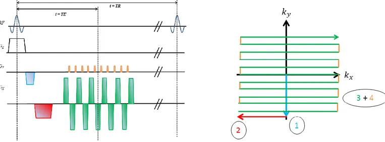
observer’s reference frame and b) the rotating reference frame. The main magnetic field is aligned with the z axis in both models. ... 6 Figure 3: Graphical depiction of the excitation process in the rotating frame when the resonance condition is met. a) At rest, the magnetization vector is aligned with the longitudinal axis of the reference frame. b) The RF pulse, oriented along the 𝒙′axis, tips the magnetization away from the 𝒛′ axis with a given flip angle. c) The excitation process allows for the decomposition of 𝑴 into its longitudinal and transverse components. ... 7 Figure 4: Graphical representation of the relationship between RF pulse bandwidth, gradient strength and slice thickness during selective excitation. ... 13 Figure 5: Graphical representation of k-space as a matrix containing M by N points, depending on the number of frequency and phase-encoding steps used to acquire an image. Each point of frequency space represents the entire signal waveform acquired at that moment using a specific combination of frequency encoding and phase encoding. Image adapted from (Huettel et al, 2014.) ... 17 Figure 6: Left – Pulse sequence diagram illustrating the principle of gradient-echo generation. Right – Corresponding trajectory drawn in k-space by the spatial encoding gradients. The process is repeated until each line of k-space is filled and a gradient echo is generated when the green line crosses the ky axis. ... 19

Figure 7: Left – Pulse sequence diagram illustrating the principle behind spin echo generation. Right – Corresponding trajectory drawn in k-space. It is important to note that the application of a 180° refocusing pulse will cause a phase reversal in frequency space, multiplying the (kx, ky)

(9)

viii

Figure 8: Picture of a neuron and its structural components. Image sourced from [1]. ... 23 Figure 9: Vascular anatomy of the arterial circulation in the neck, face and upper thorax in humans. Left – Image of the internal and carotid arteries in the neck. Right- Illustration of the Circle of Willis, basilar arteries, posterior cerebral arteries, middle cerebral arteries and

anterior cerebral arteries. Images sourced from [2] and [3]... 25 Figure 10: Graphical representation of the physiological changes brought on by functional hyperemia in the brain’s vascular network. Figure adapted from (Jezzard et al, 2005)... 28 Figure 11: Diagram of a venous blood vessel modelled as a cylinder of infinite length with a radius of R oriented at an angle θ with the main magnetic field lines. Given a susceptibility difference of Δχ between the interior of the vessel and its surroundings, a spin located at a distance r from the center of the vessel’s lumen and oriented at an angle φ from the projection of B0 into the vessel’s axial plane will experience a frequency shift given by Eq. 1.37. Figure adapted from (Kim et al, 2006; Berman, 2012) ... 30 Figure 12: Graphical representation of the magnetic field distortion pattern generated by the passage of paramagnetic deoxyhemoglobin within a blood vessel. The bright and dark regions represent regional increases and decreases of the magnetic field strength. B0 remains

undistorted along lines oriented at ± π/4. R represents the vessel’s radius. Figure adapted from (Buxton, 2009)... 32 Figure 13: Left – Pulse sequence diagram depicting GRE echo-planar imaging (EPI). Right – Corresponding k-space trajectory. EPI allows for the acquisition of the entirety of k-space in a single TR due to the successive generation of echoes produced by rapid gradient flipping. ... 37 Figure 14: Illustration of the CASL technique. a) Simplified pulse sequence of the tagging experiment used in CASL. EPI designates the readout module incorporated into the CASL sequence. b) Graphical representation of the elements used for perfusion imaging using CASL. The labelling plane is shown in orange and is positioned in a region upstream from the organ to be imaged. The image volume is shown in green. c) Simplified pulse sequence of CASL’s control experiment. The resonance frequency of the tagging pulse is adjusted to as to place the labelling plane in a region that is symmetrically opposed to its position during the tagging experiment relative to the center of the image volume, as shown in d).Figure adapted from (Debacker, 2014) ... 41

(10)

ix

Figure 15: Illustration of a PICORE-type PASL technique. a) Simplified pulse sequence diagram of the tagging experiment used in a PICORE sequence. An inversion pulse is played out with a flip angle of 180° in order to modulate the longitudinal magnetization of flowing spins in a volume located upstream from the imaging slab. EPI designates the readout module incorporated into the sequence. b) Graphical representation of the elements used for spin tagging using this sequence. The image volume is shown in green while the tagging volume is displayed in orange. c) In PICORE-type PASL, the slice-selective gradient is either turned off (as shown above) or shifted in time to prevent the inversion pulse from affecting blood water spins during the control experiment, leading to the absence of the tagging volume in d). Figure

adapted from (Debacker, 2014) ... 43 Figure 16: Illustration of a pCASL sequence’s tagging mechanism. Left - The long RF pulse and magnetic field gradient used for flow-driven adiabatic inversion of blood water spins are

respectively replaced by a train of short and equally-spaced tagging pulses and a waveform composed of slice-selection and spoiler gradients with unequal moments and alternating polarities. The average gradient strength produced at this time is similar to the gradient amplitude used in CASL. A phase increment is successively added to each tagging pulse to ensure that their phase schedule matches that of the flowing spins. EPI designates the readout module incorporated into the pulse sequence. Right- Graphical representation of the elements used for spin tagging in a pCASL sequence. The labelling plane appears in orange while the image volume is shown in green. Figure adapted from (Debacker, 2014)... 45 Figure 17: Pulse sequence diagrams of the control experiments carried out in balanced (top) and unbalanced (bottom) pCASL sequences. In the balanced variant, the gradient waveform does not change between the tagging and control measurements. The phase of each tagging pulse is incremented by the same amount as in the tagging experiment, but with an added offset term of N*π, with N representing the Nth pulse in the train. In the unbalanced conformation, the

moments of the spoiler gradients is adjusted in order to produce an average gradient strength of 0 during the control experiment. Additionally, the phase of each successive tagging pulse is made to alternate between 0° and 180° at this time. Figure adapted from (Debacker, 2014) ... 46 Figure 18: Pulse sequence diagram of the GRESE-EPI sequence developed in this work. This sequence allows for the interleaved acquisition of GRE and SE data by switching between SE-EPI and GRE-SE-EPI during odd-numbered and even-numbered measurement periods, respectively. The measurement number is given by (n+1), where n represents the current repetition and is equal to n = 0, 1, 2, …, N. It is also possible to set the TE for each imaging technique used in GRESE-EPI independently from each other. The TEs used for GRE-EPI and SE-EPI are represented by the variables TE1 and TE2. In the diagram shown above, the readout gradients are shown in green and the phase blips are orange. The gradients used for advanced phase

(11)

x

correction appear in red and the prewinders are colored blue. The slices-selection gradients are shown as line drawings, as are the crusher gradients which bracket the 180° refocusing pulse. 49 Figure 19: Examples of images acquired using GRESE-EPI for Subject 1 during a pilot fMRI scan involving a visual stimulus. The overlaid activation maps were corrected for FDR with a threshold of 0.001. 3 contiguous slices retrieved from the center of one image volume are shown here for GRE data (a, b, c) and SE data (d, e, f). The color bars indicate the t-score values and the greyscale bar indicates the signal intensity of the underlying images... 53 Figure 20: Examples of the images acquired using GRESE-EPI for Subject 2 during a pilot fMRI scan involving a visual stimulus. The overlaid activation maps were corrected for FDR with a threshold of 0.001. 3 contiguous slices retrieved from the center of one image volume are shown here for GRE data (a, b, c) and SE data (d, e, f). The color bars indicate the t-score values and the greyscale bar indicates the signal intensity of the underlying images... 53 Figure 21: Waveform of the excitation pulse originally used in GRESE-EPI. The pulse was constructed as an array of complex quantities in MATLAB using its magnitude and phase data, imported from IDEA’s RF pulse library. The amplitude of the pulse was left unscaled in this figure. ... 56 Figure 22: Slice profile of the excitation pulse used in GRESE-EPI obtained using the Bloch equation simulator developed by Dr. Brian Hargreaves. ... 57 Figure 23: Waveform of the excitation pulse created using MATPULSE. ... 60 Figure 24: Slice profile of the excitation pulse created using MATPULSE. This profile was obtained by using the Bloch equation simulator available in MATPULSE... 61 Figure 25: Slice profile of the excitation pulse created using MATPULSE. This slice profile was obtained by using the Bloch equation simulator developed by Dr. Brian Hargreaves. ... 62 Figure 26: Picture of the ACR phantom used in this thesis to obtain measurements of the width of the slice profiles destined for use in GRESE-EPI. ... 63

(12)

xi

Figure 27: Sagittal view of the ACR phantom. In order to perform a measurement of the slice thickness, the slice must be placed at the center of the yellow box shown above in order to produce an image of the signal-producing portion of the crossed ramps. ... 64 Figure 28: Close-up of the signal-producing portion of the crossed ramps, as viewed during an experiment seeking to evaluate the slice thickness. The lengths of ramps “a” and “b” are

represented by the orange and blue bars in the zoomed-in picture of the ramps. ... 64 Figure 29: Axial slices of the ACR phantom acquired using the MiniFLASH (left) and MiniSE (right) sequences with the SLR pulse as the excitation pulse. ... 67 Figure 30: Axial slices of the ACR phantom acquired using the MiniFLASH (left) and MiniSE (right) sequences harbouring the original excitation pulse used in GRESE-EPI... 67 Figure 31: Examples of the magnitude (left) and phase (right) images acquired during SWI. The images presented here were acquired using a TE of 13 ms and the phase image was processed using a binary mask of the brain to remove all noise outside the target structure. Phase wraps are also present in this image, appearing as sudden shifts in the signal intensity between

neighbouring pixels. The magnitude image was skull-stripped, as seen above, before generating the binary mask. ... 70 Figure 32: Examples of venograms generated using datasets acquired at TE = 13 ms (a) and TE = 41 ms (b), in addition to the final venogram generated by averaging 5 sets of processed SWI images acquired at different echo times. The venograms shown in this figure were acquired during the scan protocol described in section 3.1.1 for one participant. Images (a) and (b) were used to produce (c). All venograms were generated using a non-linear phase mask function as well as the adaptive filter method. ... 72 Figure 33: Envelope of a Hanning-shaped tagging pulse designed for use in a pCASL sequence. ... 74

Figure 34: Decomposition of the tagging unit’s gradient lobes into a series of geometric shapes in order to determine the value of Gspoil that will result in the application of the correct value of

(13)

xii

Figure 35: Steps taken to create a binary vein mask by using a subject’s venogram, as generated using the steps outlined in section 2.2 using the non-linear phase mask function and the adaptive filter method. The venogram, shown in a) is first thresholded using a value that was determined through visual inspection of the data in order to set the intensity of all non-venous structures to zero. This new image volume, shown in b), is then downsampled to the resolution of the

respective subject’s EPI data. The maps of the percent effect size for the same participant from which the data was obtained was used as the sampling template for this operation. The final result is shown in c). ... 82 Figure 36: Examples of the multi-value vein masks used for the analysis of brain activation. These masks were created for one individual having undergone both fMRI experiments described in section 3.1.1. The voxels belonging to the venous vasculature found within the common region of activation appear as white on the images and the voxels classified as parenchymal tissue appear in light grey. Black and dark grey voxels are either non-venous structures or vessels which are found outside the subject-specific functional ROI; the individual t-scores and percent effect size values detected in the latter regions were not considered during data analysis. ... 83 Figure 37: Examples of images acquired using GRESE-EPI during an fMRI experiment

involving a visual stimulus using optimized values for GRE-EPI and SE-EPI. (TE1 = 30 ms, TE2

= 75 ms) GRE data for subjects 1 (a), 2 (b), 3 (c) and 4 (d) are shown from left to right in the top row. SE data for subjects 1 (e), 2 (f), 3 (g) and 4 (h) are shown from left to right in the bottom row. The color bars indicate the t-score values. The greyscale bar indicates the signal intensity of the brain images. The slices shown for subject 4 do not come from the same position in the imaging slab as those shown for subjects 1, 2 and 3. ... 87 Figure 38: Examples of images acquired using GRESE-EPI during an fMRI experiment

involving a visual stimulus using matched values for GRE-EPI and SE-EPI. (TE1 = TE2 = 30 ms)

GRE data for subjects 1 (a), 2 (b), 3 (c) and 4 (d) are shown from left to right in the top row. SE data for subjects 1 (e), 2 (f), 3 (g) and 4 (h) are shown from left to right in the bottom row. The color bars indicate the t-score values. The greyscale bar indicates the signal intensity of the brain images. The slices shown for subject 4 do not come from the same position in the imaging slab as those shown for subjects 1, 2 and 3. ... 88 Figure 39: Examples of the percent effect size maps generated using each subject’s GRE and SE data acquired using GRESE-EPI during an fMRI experiment involving the use of a visual stimulus using optimized TEs for SE-EPI and GRE-EPI. The percent effect size maps generated using GRE data from subjects 1 (a), 2 (b), 3 (c) and 4 (d) are presented in the top row, from left to right. The percent effect size maps generated using SE data from subjects 1 (e), 2 (f), 3 (g) and

(14)

xiii

4 (h) are presented in the bottom row, from left to right. The color bars indicate the percent effect size values. The slices shown in this figure correspond to those shown in figure 37... 88 Figure 40: Examples of the percent effect size maps generated using each subject’s GRE and SE data acquired using GRESE-EPI during an fMRI experiment involving the use of a visual stimulus using matched TEs for SE-EPI and GRE-EPI. The percent effect size maps generated using GRE data from subjects 1 (a), 2 (b), 3 (c) and 4 (d) are presented in the top row, from left to right. The percent effect size maps generated using SE data from subjects 1 (e), 2 (f), 3 (g) and 4 (h) are presented in the bottom row, from left to right. The color bars indicate the percent effect size values. The slices shown in this figure correspond to those shown in figure 38... 89 Figure 41: Histogram of the average percent effect size detected in the venous vasculature and parenchymal tissue in a common region of activation for data acquired using GRE-EPI and SE-EPI with the GRESE-SE-EPI pulse sequence using optimal TEs for both acquisition techniques in an fMRI scan involving a visual stimulation paradigm. The error bars represent the standard

deviation and data from subjects 2, 3 and 4 were used to compute the average values. ... 90 Figure 42: Histogram of the average percent effect size detected in the venous vasculature and parenchymal tissue in a common region of activation for data acquired using GRE-EPI and SE-EPI with the GRESE-SE-EPI pulse sequence using matched TEs for both acquisition techniques in an fMRI experiment involving a visual stimulation paradigm. The error bars represent the standard deviation and data from subjects 2, 3 and 4 were used to compute the average values. ... 90

Figure 43: Histogram of the average t-score detected in the venous vasculature and

parenchymal tissue in a common region of activation for data acquired using GRE-EPI and SE-EPI with the GRESE-SE-EPI pulse sequence using optimal TEs for both acquisition techniques in an fMRI scan involving a visual stimulation paradigm. The error bars represent the standard deviation and data from subjects 2, 3 and 4 were used to compute the average values. ... 92 Figure 44: Histogram of the average t-score detected in the venous vasculature and

parenchymal tissue in a common region of activation for data acquired using GRE-EPI and SE-EPI with the GRESE-SE-EPI pulse sequence using matched TEs for both acquisition techniques in an fMRI experiment involving a visual stimulation paradigm. The error bars represent the standard deviation and data from subjects 2, 3 and 4 were used to compute the average values. ... 92

(15)

xiv

Figure 45: Histogram of the average gray matter, white matter and whole-brain CBF for all 3 subjects computed using data acquired with the in-house (MNI) pCASL sequence and the

externally-developed pCASL sequence. The error bars represent the standard deviation. ... 95 Figure 46: Examples of images acquired using the pCASL sequence developed in this work for 3 subjects (top row) along with the corresponding CBF maps. (bottom row) One pair of images is shown for subjects 1 (a, d), 2 (b, e) and 3 (c, f). The greyscale bars indicate the signal intensity of the EPI data while the color bar indicates the values of CBF in units of ml/100g/min. ... 96 Figure 47: Examples of images acquired using an externally-developed pCASL sequence for 3 subjects (top row) along with the corresponding CBF maps. (bottom row) One pair of images is shown for subjects 1 (a, d), 2 (b, e) and 3 (c, f). The greyscale bars indicate the signal intensity of the EPI data while the color bar indicates the values of CBF in units of ml/100g/min. ... 97

(16)

xv

List of tables

Table 1: Table of the scan parameters used for the pilot experiments involving GRESE-EPI .... 51 Table 2: Table of the scan parameters used for the MiniFLASH and MiniSE pulse sequences used in experiments seeking to measure the slice thickness associated with the excitation and the refocusing pulses used in GRESE-EPI... 66 Table 3: Table of the values of the slice thickness calculated using each pairing of excitation and refocusing pulses using the ACR phantom method. ... 68 Table 4: Table of the scan parameters used to test the pCASL sequence’s imaging capabilities in the context of a whole-brain CBF quantification experiment at rest... 84 Table 5: Table of the average gray matter, white matter and whole-brain CBF in 3 subjects using the pCASL sequence developed in this work and an externally-developed pCASL sequence. The standard deviation is shown here as the error term. These values were obtained using a set of analysis scripts created by Dr. Clément Debacker... 94

(17)

xvi

List of abbreviations

AAPM: American Association of Medical Physicists

AC-PC: Anterior commissure – Posterior commissure

ACR: American College of Radiology

ADC: Analog-to-digital converter

ASL: Arterial spin labelling

ATP: Adenosine triphosphate

BET: Brain extraction tool

BOLD: Blood oxygen level-dependent

CASL: Continuous arterial spin labelling

CBF: Cerebral blood flow

CBV: Cerebral blood volume

CMRglu: Cerebral metabolic rate of glucose

CMRO2: Cerebral metabolic rate of oxygen

CNR: Contrast-to-noise ratio

DSC: Dynamic susceptibility contrast

EPI: Echo planar imaging

EPISTAR: Echo planar imaging and signal targeting with alternative radiofrequency

FAIR: Flow-sensitive alternating inversion recovery

FAST: FMRIB’s automatic segmentation tool

FID: Free induction decay

FLASH: Fast low angle shot

fMRI: Functional magnetic resonance imaging

FWHM: Full width at half-maximum

GRE: Gradient-recalled echo

MPRAGE: Magnetization-prepared rapid gradient echo

MRI: Magnetic resonance imaging

PASL: Pulsed arterial spin labelling

pCASL: Pseudo-continuous arterial spin labelling

PICORE: Proximal inversion with a control for off-resonance effects

PLD: Post-label delay

Q2TIPS: QUIPSS II with thin-slice TI1 periodic saturation

QUIPSS II: Quatitative imaging of perfusion using a single subtraction

RF: Radiofrequency

ROI: Region of interest

SAR: Specific absorption rate

SE: Spin-echo

SLR: Shinnar-LeRoux

SNR: Signal-to-noise ratio

SWI: Susceptibility-weighted imaging

T: Tesla

T1: Longitudinal relaxation time

T2: Transverse relaxation time

T2*: Effective transverse relaxation time

TE: Echo time

TI: Inversion time

(18)

xvii

Introduction

Due to its ability to non-invasively produce high-resolution images of the human body with multiple types of contrasts in order to visualize biological structures of interest, magnetic resonance imaging (MRI) is often considered as one of the most important diagnostic tools in the field of medicine. However, its use is not restricted to anatomical imaging; discoveries made in the early 1990s have made it possible to use this modality to qualitatively and quantitatively probe brain physiology. (Ogawa et al, 1993) Numerous biological and physical phenomena in the human body make the detection of neuronal activity in the brain using MRI possible, such as neurovascular coupling, functional hyperemia and the changing magnetic properties of hemoglobin, the latter of which depend on the oxygenation state of this protein. These phenomena all contribute to the generation of what is known as blood oxygenation level-dependent or “BOLD” contrast in MRI. (Huettel et al, 2014)

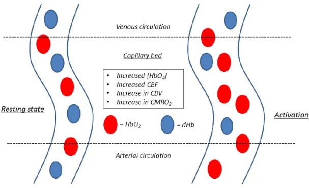
During periods of brain activity, neurons will generate bioelectrical signals known as action potentials in order to engage in information processing and cell signalling. (Marieb, 2005) The creation of these signals will trigger molecular cascades that culminate in the release of factors that act upon the smooth muscle cells surrounding blood vessels proximal to the site of increased synaptic activity in an effort to regulate regional blood flow in the cerebral cortex. (Atwell et al, 2010) The net effect of this regulatory process is a large increase in cerebral blood flow towards the region of neuronal activation, a physiological process also known as functional hyperemia, as well as increases in the cerebral metabolic rates of glucose and oxygen consumption, which denote the utilization of nutrients necessary for cellular respiration and the production of adenosine triphosphate by neurons. The latter step ensures the continuation of signalling activities carried out by these cells. (Kim et al, 2006)

However, a quantity of oxygen that far surpasses the metabolic needs of the neurons is delivered to brain parenchyma at this time. (Fox et al, 1986) This phenomenon arises due to functional hyperemia and is responsible for driving out deoxyhemoglobin from the venous vasculature during periods of neuronal activation. This is of profound importance in functional magnetic resonance imaging (fMRI) as the differences between the magnetic properties of deoxygenated hemoglobin and the surrounding parenchymal tissue will generate magnetic field

(19)

xviii

distortions both in and around the blood vessels, which are in turn responsible for a hastened regional decay of MRI signal. (Kim et al, 2006) As deoxyhemoglobin is replaced by its oxygenated counterpart, the size of these distortions will get smaller and the longevity of regional MRI signal will increase, which translates to an increase of signal intensity at this location on the final image. This relationship between blood oxygen content and signal intensity is what gives the BOLD contrast its name.

Many different imaging techniques can be used to acquire images presenting BOLD contrast with fast imaging techniques such as echo planar imaging (EPI) being widely utilized due to the need for rapid collection of functional data. In particular, gradient-echo EPI (GRE-EPI) stands out as a particularly viable imaging method in BOLD fMRI due to its sensitivity to the field distortions generated by the presence of paramagnetic magnetic field perturbers such as deoxyhemoglobin. However, GRE-EPI will detect signal variations associated with fluctuations of the concentration of this protein in all types of blood vessels, from capillaries to large draining veins. (Harmer et al, 2012) This reduces its spatial specificity as it is accepted that only changes that take place in the microvasculature are specific to the sites of neuronal activity.

To tackle this issue, spin-echo EPI (SE-EPI) has been proposed as an alternative technique for BOLD fMRI experiments. This technique employs a radiofrequency pulse that eliminates the effects of magnetic field distortions around large vessels while still remaining sensitive to variations of deoxyhemoglobin levels in the microvasculature. This is due to the different molecular mechanisms implicated in the deoxyhemoglobin-mediated signal decay at two different scale sizes. The elimination of these effects, however, reduces the sensitivity of SE-EPI to BOLD signal as the changes in signal intensity arising from the capillaries are smaller than those generated by large vessels in the venous vasculature. (Budde et al, 2014)

Perfusion imaging can also be employed as an alternative to BOLD fMRI to detect neuronal activity in the cerebral cortex due to the relationship of linear proportionality between blood flow and the cerebral metabolic rate of glucose. (Faro et al, 2011) Arterial spin labelling (ASL) is commonly employed for this purpose and its mode of operation rests on the use of radiofrequency pulses to invert the magnetization of flowing blood water in the brain’s feeding arteries in the neck and acquiring an image of the brain after a short delay to allow this tagged volume of blood to diffuse into the brain’s extravascular space. (Wong, 2014)

(20)

xix

A second measurement of the brain is subsequently acquired without blood tagging and the pairwise subtraction of these two images results in a difference in the magnetization which is proportional to the value of blood flow. ASL can be implemented in either a pulsed or continuous configuration, (PASL and CASL) depending on whether a long RF pulse is used to continuously invert blood water through a flow-driven process or if a short RF pulse is employed to tag all of the blood water in a given volume proximal to the imaging region. (Alsop et al, 2015) Recently, ASL sequences featuring a pseudo-continuous tagging mechanism have also been developed in order to combat the disadvantages associated with both PASL and CASL while conserving each technique’s respective advantages. The pCASL sequence tags blood water using a flow-driven process similar to CASL in which the long radiofrequency pulse is replaced by a train of shorter and equally-spaced tagging pulses. (Wu et al, 2007; Dai et al, 2008)

In this thesis, two MRI pulse sequences were developed in order to study the generation of BOLD contrast using GRE-EPI and SE-EPI as well as to perform perfusion imaging in humans at rest. The first of these two sequences was an EPI sequence permitting the interleaved acquisition of functional data using both GRE-EPI and SE-EPI (GRESE-EPI) during a single scan session while the second was a pCASL pulse sequence operating in an unbalanced configuration. To validate the functionality of the GRESE-EPI sequence developed herein and to compare the performances of both types of EPI presented in this introduction, it was deployed in the context of a BOLD fMRI experiment involving a visual stimulation paradigm using optimal and matched echo times for both acquisition techniques. The assessment of the pCASL sequence’s functionality was accomplished through a CBF quantification experiment in which values of blood flow were calculated in gray matter, white matter and in the whole brain in healthy adults at rest. These values were then compared to those obtained using an externally-developed pCASL sequence during the same scan session. This sequence was considered as a “gold standard” due to its proven efficacy in perfusion experiments carried out in vivo. (Tancredi et al, 2015) Other steps taken to design the pulse sequences described in this thesis, such as the design of radiofrequency pulses for combined GRE and SE imaging, as well as the steps taken to develop the tools needed for data analysis, such as the generation of cerebral venograms using susceptibility-weighted imaging for the evaluation of BOLD signal generation in the venous vasculature, will be presented in this thesis.

(21)

1

Chapter 1. Theoretical framework

In this chapter, the theoretical notions underpinning the phenomena central to this thesis will be introduced and explained in three sections. The first of these will be devoted to the particle physics that make magnetic resonance imaging (MRI) possible. In the second section, the processes by which images are created using MRI, such as slice selection, spatial encoding of MRI signals, creation of signal echoes and contrast generation, will be subject to exposition. In the third and final section, the topic of functional MRI (fMRI) will be broached. Two functional contrasts, perfusion contrast and blood oxygenation level-dependent (BOLD) contrast, will be studied in addition to commonly used imaging techniques employed in experiments in which these types of activation signals are studied.

1.1 Particle physics

MRI chiefly rests on the excitation of biological tissues placed in a strong magnetic field using radiofrequency (RF) waves. These RF pulses will perturb the orientation of protons in said tissues and this excitation process is responsible for signal generation. This signal will then be detected using a receiver coil as an induced electromotive force. Many other factors are involved in the imaging process, but before delving into their specifics, it is necessary to present the fundamental characteristics of atoms suitable for use in MRI as well as how they interact with various magnetic fields at the atomic and molecular levels.

1.1.1 Spin angular momentum and magnetic moment

Hydrogen H1 atoms, referred to as protons in this work, are the main source of MRI signal in conventional body scans. This is due to its abundance in biological tissues, appearing in the form of water molecules. However, many other elements can be targeted in the context of MRI or magnetic resonance spectroscopy (MRS) experiments, such as fluorine 19F, phosphorus 31_{P and even sodium}23_{Na, in order to achieve a better understanding of various physiological}

(22)

2

processes involved in homeostasis as well as in various pathologies. (Ruiz-Cabello et al, 2011; Ouwerkerk, 2011; Sabouri, 2014)

Not every atom can be targeted using MRI or MRS. Only atoms whose nuclei are made up of an odd number of either protons or neutrons exhibit the necessary properties which make them viable for these experiments. Specifically, the composition of an atom’s nucleus will determine whether or not the atom possesses spin angular momentum. This quantity is represented by S in equation 1.1:

𝑆 = (ℎ

2𝜋

) 𝑚

𝑠 (1.1)

In the equation above, h represents Planck’s constant and ms designates a quantum

number which represents the atom’s spin state. For protons and neutrons, ms can take one of two

values: ± ½. For atoms whose nuclei contain an even number of both nucleons, the values of ms

taken by all protons and neutrons will cancel out, bestowing upon the atom a net angular momentum of zero (S = 0.) This consequently prevents the element’s use in MRI.

Protons, due to their electric charge and their non-null spin angular momentum, also possess a magnetic moment. This quantity, usually represented by μ, can be expressed as the product of S and the gyromagnetic ratio, γ:

𝜇 = 𝛾𝑆

(1.2)

The gyromagnetic ratio is a constant unique to every atom and is equal to 42.58 MHz/T for hydrogen 1H. Due to their angular momentum, protons are also referred to as “spins” or “water spins” in the context of anatomical and functional MRI.

1.1.2 Magnetization vector

In the absence of a static magnetic field, i.e. a magnetic field which is invariant in time and space, protons exist in a degenerate state; these particles occupy the same energy stratum, regardless of what their spin angular momentum and magnetic moment may be. When a magnetic field fitting this description is applied to spins, as is the case in an MRI scanner,

(23)

3

Zeeman splitting occurs. Depending on their ms values, protons will be divided into two distinct

populations occupying two separate energy strata. (Huettel et al, 2014) The potential energy of protons in each one of these populations depends on not only ms, but also on the gyromagnetic

ratio and the external magnetic field’s strength, represented by B0 in equation 1.3:

𝐸 = −𝛾 (ℎ

2𝜋) 𝑚𝑠𝐵0 (1.3)

Using the Boltzmann distribution, it is also possible to obtain a ratio of the sizes of the two proton populations:

𝑃𝑒− 𝑃𝑒+

= 𝑒

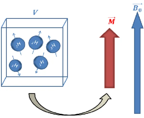
∆𝐸 𝑘_𝑏𝑇 ⁄ (1.4)

Solving equation 1.4 reveals that while both populations are nearly equal in size, the low-energy proton population is slightly larger than its high-low-energy counterpart. This mismatch between population sizes leads to the sample becoming slightly magnetized at the macroscopic level. (Nishimura, 2010) This net magnetization is usually represented as a vector (𝑀⃑⃑ ) whose magnitude can be expressed as the sum of all magnetic moments within a given volume V:

𝑀

⃑⃑ =

1

𝑉

∑ 𝜇

(1.5)

It is also possible to represent both proton populations as being aligned with or against the magnetic field lines. In this model, the low-energy population corresponds to the protons aligned with the field lines; it is energetically advantageous for these particles to adopt this conformation, thus leading to the aforementioned mismatch between proton population sizes. For this reason, the magnetization vector is also oriented parallel to the external magnetic field. (Huettel et al, 2014)

Protons, as well as 𝑀⃑⃑ , do not remain static under the influence of a static magnetic field. Due to their angular momentum and their magnetic moment, protons will begin to rotate around the magnetic field lines in a manner reminiscent of a spinning top. This form of rotation is also known as precession. Protons undergo precession at a specific frequency, named “Larmor frequency,” which depends on γ as well as on the magnetic field’s strength.

(24)

4

Figure 1: Graphical representation of the magnetization vector 𝑴⃑⃑⃑ arising from a given volume V. The sample

becomes magnetized in the presence of an external static magnetic field B0 due to a surplus of protons aligned with the magnetic field lines.

1.1.3 Larmor frequency and nuclear magnetic resonance

The laws of classical mechanics can be used to derive a mathematical expression allowing for the computation of an atomic element’s Larmor frequency. Any particle possessing angular momentum and a magnetic moment will experience torque when placed in a magnetic field, as described by equation 1.6:

𝜏 = 𝜇 ⃑⃑⃑ × 𝐵⃑⃑⃑⃑ ₀ (1.6)

This torque can also be expressed as a variation of the angular momentum over time. The resulting cross product can be written as:

𝑑𝑆

𝑑𝑡 = 𝜇 ⃑⃑⃑ × 𝐵⃑⃑⃑⃑ 0 (1.7)

By multiplying both sides of equation 1.7 by γ, it becomes possible to express the variation of the magnetic moment over time:

𝑑𝜇

𝑑𝑡 = 𝛾(𝜇 ⃑⃑⃑ × 𝐵⃑⃑⃑⃑ ) 0 (1.8)

Equation 1.8 is also valid at the macroscopic level and can be extended to the magnetization vector:

(25)

5 𝑑𝑀⃑⃑

𝑑𝑡 = 𝛾(𝑀 ⃑⃑⃑⃑ × 𝐵⃑⃑⃑⃑ ) 0 (1.9)

By solving this differential equation, which governs the rate of change of the magnetization vector over time, the relationship between the Larmor frequency and the magnetic field strength is obtained:

𝜔₀= 𝛾𝐵₀ (1.10)

The Larmor frequency is of great import when attempting to discuss proton excitation. As mentioned at the beginning of this chapter, MRI signal is generated by using an RF pulse to alter the orientation of protons in a targeted volume. This is done to tip the magnetization vector away from the external magnetic field’s lines, as 𝑀 ⃑⃑⃑⃑ cannot be distinguished from 𝐵⃑ ₀ under normal circumstances. In order for excitation to occur, however, the central frequency of the RF pulse must be matched to the protons’ Larmor frequency. When this condition, also known as the resonance condition, is met, energy is transferred from the RF pulse to the sample, prompting a number of protons on the lower energy stratum to ascend to the higher level. (Berman, 2012) At the macroscopic level, this corresponds to the magnetization vector moving away from 𝐵⃑ ₀ and into a plane orthogonal to the magnetic field lines.

1.1.4 Principles of excitation

It is also possible to explain the excitation process by making use of classical mechanics notions. From this point of view, the magnetization vector’s descent into the transverse plane is due to the application of torque by the RF pulse. This pulse is a circularly-polarized electromagnetic wave whose magnetic field can be expressed as:

𝐵⃑ ₁ = 𝐵₁𝑥̂ cos(𝜔𝑡) − 𝐵₁𝑦̂ sin(𝜔𝑡) (1.11) As 𝐵⃑ ₁’s central frequency is the same as the protons’ precession frequency in the case of on-resonance excitation, it becomes possible to describe the interaction between the RF pulse and the magnetization vector in a rotating reference frame. The differences between this new model and the observer’s reference frame are illustrated in figure 2, but the main advantage of

(26)

6

this new notation scheme is that 𝑀 ⃑⃑⃑⃑ , while still aligned with 𝐵⃑ ₀, can be considered static instead of undergoing precession.

Figure 2: Graphical representation of the behaviour of the magnetization vector in a) the observer’s reference frame and b) the rotating reference frame. The main magnetic field is aligned with the z axis in both models.

Equations 1.12a, 1.12b and 1.12c describe the passage from one reference frame to the other:

𝑥̂′ _{= 𝑥̂ cos(𝜔𝑡) − 𝑦̂ sin(𝜔𝑡)} _(1.12a) 𝑦̂′ = 𝑥̂ cos(𝜔𝑡) + 𝑦̂ sin(𝜔𝑡) (1.12b)

𝑧̂′ _{= 𝑧̂} _(1.12c)

The RF pulse’s effect on the net magnetization of the spin system can be described using a differential equation analogous to equation 1.9:

𝑑𝑀⃑⃑ _𝑟𝑜𝑡

𝑑𝑡 = 𝛾(𝑀⃑⃑ 𝑟𝑜𝑡× 𝐵⃑ 𝑒𝑓𝑓) (1.13)

In the equation above, the magnetic field term, 𝐵⃑ _𝑒𝑓𝑓, encompasses not only the contribution of the RF pulse’s magnetic field, 𝐵⃑ ₁, but also that of the main magnetic field 𝐵⃑ ₀. This new variable is dubbed the effective magnetic field and is described by equation 1.14:

𝐵⃑ _𝑒𝑓𝑓 = 𝐵₁𝑥̂′ + (𝐵₀−𝜔

(27)

7

In the case of on-resonance excitation, the longitudinal component of the effective field, i.e. the field component aligned with the z’ axis of the rotating reference frame, is reduced to zero and the RF pulse’s effect on 𝑀⃑⃑ is maximized. The magnetization vector will then pivot around the x’ axis, as depicted in figure 3, at an angle which depends on the RF pulse’s maximum amplitude, the duration of its application, designated by τ in equation 1.15, and the protons’ gyromagnetic ratio:

𝜃 = 𝛾𝐵₁𝜏 (1.15)

Figure 3: Graphical depiction of the excitation process in the rotating frame when the resonance condition is met. a) At rest, the magnetization vector is aligned with the longitudinal axis of the reference frame. b) The RF pulse, oriented along the 𝒙̂′axis, tips the magnetization away from the 𝒛̂′ axis with a given flip angle. c) The excitation process allows for the decomposition of 𝑴⃑⃑⃑ into its longitudinal and transverse components.

The transverse component of the magnetization vector, Mxy, can also be broken down into two more components respectively oriented along the x’ and y’ axes: Mx and My. Complex

notation is commonly employed to represent the composition of this transverse component of the magnetization vector:

𝑀_𝑥𝑦(𝑡) = 𝑀_𝑥(𝑡) + 𝑖𝑀_𝑦(𝑡) (1.16) The angle separating these two components is known as the phase angle and plays an important role in characterizing MRI signal behaviour:

𝜑 = tan−1₍𝑀𝑦

(28)

8

It is important to reiterate at this point that the net magnetization of a spin system cannot be detected unless it is tipped into the magnetic field’s transverse plane; only the transverse component of the magnetization vector contributes to signal generation.

1.1.5 Relaxation mechanisms

Once excitation ceases, the system will begin to return to equilibrium through two relaxation mechanisms which govern the longitudinal magnetization’s recovery rate and the transverse component’s decay. These processes operate according to time constants which vary from one biological tissue to the next, but the molecular interactions at the heart of these phenomena are the same in every case.

The regrowth of the magnetization vector’s longitudinal component is due to the dissipation of energy transferred to the protons by the RF pulse into the surrounding molecular lattice. (Berman, 2012) This process, known as longitudinal relaxation or spin-lattice relaxation, is governed by the T1 time constant and can be described by a first-order differential equation:

𝑑𝑀_𝑧

𝑑𝑡

=

−(𝑀_𝑧0−𝑀₀)

T1

(

1.18)

By solving the equation above, it becomes possible to calculate the magnitude of the longitudinal magnetization at a given time t following the excitation period:

𝑀𝑧(𝑡) = 𝑀0+ (𝑀𝑧0− 𝑀0)𝑒(−𝑡 T1⁄ ) (1.19) Transverse magnetization decay, on the other hand, is caused by a loss of phase coherence brought on by naturally-occurring interactions between neighbouring spins. (Nishimura, 2010) These interactions are responsible for transient local variations in the magnetic field strength, which in turn influence the Larmor frequency of the surrounding spins, causing them to accumulate differing amounts of phase. This phenomenon, also called spin-spin relaxation or transverse relaxation, is governed by the T2 constant and can also be described as a first-order differential equation:

(29)

9

𝑑𝑀𝑥𝑦

𝑑𝑡

=

−𝑀𝑥𝑦

T2

(1.20)

The solution to this equation, in the case of a static and uniform B0 is:

𝑀𝑥𝑦(𝑡) = 𝑀𝑥𝑦0𝑒(−𝑡 T2⁄ −𝑖𝜑) (1.21) Molecular interactions are not the only contributors to transverse relaxation. Magnetic field inhomogeneities accelerate the dephasing process that leads to transverse magnetization decay. The non-uniformity of the main magnetic field can be attributed to improper shimming or even the heterogeneous chemical composition of the object to be scanned. In the latter case, field inhomogeneities are generated when structures presenting different values of magnetic susceptibility are juxtaposed. (Huettel et al, 2014) This is particularly evident at air-tissue boundaries within the human body, in locations such as the ear canals or regions proximal to the brain’s frontal lobe. (Uludag et al, 2005)

Spins located in these regions will precess at rates which depend on the local magnetic field strength, thus impacting their phase accrual and hastening the loss of phase coherence between all spins. The resulting shortened relaxation time is governed by a new time constant, T2*, whose value can be determined by the following equation:

1 T2∗

=

1 T2

+

1 T2′

(1.22)

The effects of field inhomogeneity-induced dephasing are contained in the term 1/T2’, also referred to as R2’. This form of dephasing is noteworthy due to the fact that it is reversible; using certain imaging techniques, it is possible to reverse the loss of phase coherence prompted by susceptibility-induced field gradients, leading to a recovery of MRI signal in the affected regions. These techniques and their relevance in functional imaging will be detailed in the following sections of this chapter. The effects of pure T2 relaxation, on the other hand, are irreversible due to the random nature of the molecular interactions which generate microscopic fluctuations of the static magnetic field’s strength. (Buxton, 2013)

(30)

10

1.1.6 Bloch equation

By combining equations 1.9, 1.18 and 1.20, it becomes possible to mathematically characterize the magnetization vector’s behaviour in the presence of a magnetic field:

𝑑𝑀⃑⃑ 𝑑𝑡 = 𝑀⃑⃑ × 𝛾𝐵⃑ 0 − (𝑀_𝑥𝑥̂+𝑀𝑦𝑦̂) T2 − (𝑀_𝑧−𝑀0)𝑧̂ T1 (1.23)

This equation is called the Bloch equation and can be solved in many different ways depending on the nature of the existing magnetic fields. In the previous sub-section, one such solution has been offered to describe the behaviour of transverse magnetization arising from a perfectly homogeneous object placed within a perfectly uniform static magnetic field. In practice, these conditions are not achievable and a spatially-varying field must be considered when solving the Bloch equation. (Nishimura, 2010) In addition to this, time-varying magnetic field gradients, generated by the scanner’s gradient coils, are employed during the scan process for slice selection and spatial encoding of MRI signals. Their presence must also be accounted for when attempting to model the magnetization vector’s behaviour.

A generic solution to the Bloch equation, i.e. when a time-varying non-uniform magnetic field is considered, can be represented as:

𝑀(𝑟, 𝑡) = 𝑀(𝑟)𝑒(−𝑡 𝑇2⁄ (𝑟))_𝑒−𝑖𝜑_𝑒−𝑖𝛾 ∫ 𝐺 (𝜏)∙𝑟 𝑑𝜏₀𝑡 _(1.24) Only T2 relaxation is considered in the signal decay term and 𝐺 (𝜏) ∙ 𝑟 represents a linear, time-varying magnetic field gradient with an arbitrary orientation. (Nishimura, 2010) Here, 𝑟 represents a vector with components of arbitrary length oriented in the x, y and z directions. If only the behaviour of the magnetization vector’s transverse component is considered during signal acquisition, the total amount of signal produced by excited spins within a given volume can be expressed as:

(31)

11

1.2 Imaging principles

This section will be dedicated to describing the different processes by which an image is created using MRI, from signal detection methods to the aforementioned spatial encoding techniques. Signal echo production techniques and the contrast-generating mechanisms that make use of these echoes will also be discussed.

1.2.1 Signal detection

To understand how signal is detected in MRI, it is necessary to consider the magnetization vector’s behaviour in the observer’s reference frame following excitation. Once tipped into the transverse plane by an RF pulse, the net magnetization of a spin system will begin to die off in the transverse plane while continuing to precess around the reference frame’s longitudinal axis. In this situation, the transverse magnetization’s behaviour can be likened to that of a rotating bar magnet. (Huettel et al, 2014) A receiver coil can then be used to measure the temporal variation of magnetic flux caused by the rotation of the spin system’s magnetization. As per Faraday’s law of induction, such a variation will induce an electromotive force in a loop of wire made of a conductive metal:

𝜀 = −𝑑𝜑

𝑑𝑡 (1.26)

In order to detect the spin system’s magnetization, however, the receiver coil must be tuned to the same frequency characterizing the precession of the targeted spin species. (Sabouri, 2014)

1.2.2 Selective excitation

When a substance of homogenous composition (e.g. a bottle of distilled water) is exposed to a perfectly uniform static magnetic field, all of the spins in the sample will precess at the same Larmor frequency. Consequently, the totality of these particles will be excited by an RF pulse whose central frequency satisfies the resonance condition. In conventional scan sessions, it is

(32)

12

preferable to restrict one’s analysis to a specific region of the sample. In fMRI experiments targeting the brain, for example, the RF pulse must only excite protons in a subject’s cranial region. The key to performing selective excitation in MRI lies in equation 1.10, which describes the directly proportional relationship between magnetic field strength and the Larmor frequency. If it becomes possible to introduce a controlled variation of 𝐵⃑ ₀’s magnitude in space, a relationship between a spin’s position and its Larmor frequency can be established. To perform this operation, every MRI scanner is equipped with three pairs of gradient coils which are capable of generating linearly-varying magnetic fields in all directions of three-dimensional space. (Prince et al, 2006) These linear field gradients are then superposed onto 𝐵⃑ ₀ and the resulting magnitude at a given point is given by:

𝐵(𝑟) = 𝐵₀+ (𝐺 ∙ 𝑟 ) (1.27)

In practice, a single one of these gradients can be used to obtain images of the object in the axial, coronal or sagittal planes depending on which gradient is used. As the human body is usually aligned with the magnetic field lines, i.e. the z-axis, when placed in the scanner, equation 1.27 can be rewritten to obtain:

𝐵(𝑧) = 𝐵₀+ 𝐺_𝑧𝑧 (1.28)

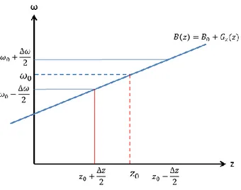
The RF pulse’s central frequency can then be adjusted to excite a specific region of the object. Each excited region, known as a slice or slab, will also have a thickness which depends on the gradient’s strength as well as on the pulse’s bandwidth, the latter representing the range of Larmor frequencies targeted during excitation. The relationship between these variables is expressed in equation 1.29 and illustrated on figure 4:

∆𝑧 = ∆𝜔

𝛾𝐺_𝑧 (1.29)

Selective excitation also allows for a simplification of equation 1.25 by reducing the signal equation to a two-dimensional problem. This is first accomplished by integrating the net magnetization along the direction orthogonal to the image plane (e.g. the z-axis for an axial image):

(33)

13

𝑀(𝑥, 𝑦) = ∫𝑧0+ 𝑀_𝑥𝑦0(𝑥, 𝑦, 𝑧)𝑑𝑧

∆𝑧 2

𝑧0−∆𝑧₂ (1.30)

The integral boundaries are set to correspond to those of the volume or slice of interest. (Nishimura, 2010) Inserting the left-hand term of equation 1.30 into equation 1.25 results in

𝑆(𝑡) = ∫ ∫ 𝑀(𝑥, 𝑦)𝑒𝑦 −𝑖𝛾 ∫ (𝐺0𝑡 𝑥(𝜏)𝑥+𝐺𝑦(𝜏)𝑦)𝑑𝜏𝑑𝑥𝑑𝑦

0 𝑥

0 (1.31)

This reduction in complexity will serve to highlight a fundamental mathematical relationship which links signal acquisition to image creation later on in this chapter.

Figure 4: Graphical representation of the relationship between RF pulse bandwidth, gradient strength and slice thickness during selective excitation.

1.2.3 RF pulses and slice profiles

The RF pulse’s central frequency and bandwidth play an important role in determining the location where excitation occurs in the sample and the resulting slice’s thickness, but they are not the only factors at play during selective excitation. The pulse’s envelope function, B1(t),

helps determine the shape of the slice profile. The ideal slice profile should be that of a boxcar function; a rectangular profile ensures that all spins whose Larmor frequencies are within the specified frequency band will be excited uniformly while those whose precession rates are outside this range of values will remain unaffected by the pulse.

(34)

14

Due to excitation being discussed in terms of frequency ranges, it is important to keep in mind that these slice profiles are defined in the frequency domain; the RF pulse’s envelope function, B1(t), must be calculated in the time domain. To retrieve the requisite envelope shape,

the inverse Fourier transform of the function that describes the slice profile can be calculated. However, the assumption that envelope functions and slice profiles are related to each other by the Fourier transform is valid only when RF pulses are played out using small flip angles (θ < 90°). This approximation breaks down for larger flip angles due to the non-linearity of the Bloch equations. The Fourier transform, being a linear operator, is ill-suited for the computation of the slice profiles associated with these pulses. (Bernstein et al, 2004):

For pulses respecting the small flip angle approximation, a rectangular slice profile can be obtained by making B1(t) a sinc function:

𝐵₁(𝑡) = 𝐴 ∗ 𝑠𝑖𝑛𝑐 (𝜋𝑡

𝑡0) = 𝐴 ∗ 𝑡0∗

𝑠𝑖𝑛(𝜋𝑡 𝑡⁄ 0)

𝜋𝑡 (1.32)

In the equation above, t0 is equal to the time separating the central lobe’s peak to the first

point of zero-crossing and is inversely proportional to the pulse’s bandwidth. As the duration of the sinc pulse’s central lobe diminishes, the range of frequencies affected by the rectangular slice profile grows. In practice, it is not possible to achieve a perfectly rectangular slice profile, as this would require the use of a sinc function of infinite duration. Truncated waveforms must therefore be used when designing RF pulses, a limitation that will affect the slope of the transition band in the pulse’s frequency response. The transition between the area targeted by the pulse and its surroundings, regions respectively referred to as the passband and the rejection band, is therefore done gradually, leading to undesirable perturbation of the spin system’s magnetization outside the targeted slice. (Bernstein et al, 2004)

More sophisticated algorithms for the production of RF pulses for specific applications in MRI are also available, such as the Shinnar-LeRoux (SLR) algorithm. Using the SLR algorithm, RF pulse creation can be thought of as a filter design process whereby B1 is determined using the

knowledge of the shape of the pulse’s frequency response. (Pauly et al, 1991) Two complex polynomials, A(z) and B(z), are required for this process. The first polynomial, B(z), is computed using finite-impulse response (FIR) filter design methods to create a frequency response whose shape best approximates that of an idealized version that is set to sin(θ/2), with θ being equal to

(35)

15

the flip angle with which the pulse is to be played out. (Pauly, 2006) Due to the finite length of the RF pulse, the filter’s shape will contain ripples in the passband and in the rejection band in addition to presenting a sloped transition band. The second polynomial, A(z), is computed using B(z) and must satisfy a normalization constraint. It has been found that the optimal solution to this problem is to select A(z) with a minimum phase, as this corresponds to the RF pulse which deposits the least amount of energy into the sample during its application. (Pauly et al, 1991; Bernstein et al, 2004) Once A(z) and B(z) have been determined, an inverse SLR transform is used to obtain the shape of the desired RF pulse in the time domain.

1.2.4 Frequency encoding

To create images using MRI, it is not enough to simply acquire the signal produced by selective excitation. It is necessary to spatially encode MRI signals in order to determine the spatial distribution of the magnetization at every point with coordinates (x, y) in the slice. The number of points to examine corresponds to the number of volume elements, or voxels, that make up the resulting image. Two mechanisms involving the use of magnetic field gradients are used for this purpose: frequency encoding and phase encoding. (Huettel et al, 2014)

As indicated by its name, frequency encoding seeks to resolve the spatial distribution of proton density along one axis of the imaging plane through the application of a magnetic field gradient during the signal detection period. As evidenced by equations 1.10 and 1.28, the introduction of a controlled variation of the magnetic field’s strength along one direction of space makes it possible to determine a spin’s position along this same axis based on its Larmor frequency. This spatial encoding process therefore makes it possible to associate a signal’s amplitude to the voxel from which it originated due to the magnetization vector formed by the spins in each voxel along the frequency axis being characterized by a unique value of the Larmor frequency, as expressed by the relationship of linear proportionality between this quantity and the magnetic field strength. An analog-to-digital converter (ADC) is also used at this time to discretely sample the signal as it is being acquired. Due to the frequency-encoding gradient being deployed at the same time as the ADC, the former is also known as a readout gradient. (Huettel et al, 2014)