•
•
•
•
•
•
•
•
•
•
•
•
•
•
•
•
•
•
•
•
•
•
•
•
•
•
•
•
•
•
•
•
•
•
•
•
•
•
•
•
•
•
•
•
INTEGRATION OF A TOPOGRAPHIC
INDEX IN THE HYDROLOGY
COMPONENT OF THE INDICATOR OF
RISK OF WATER CONTAMINATION BY
PHOSPHORUS
•
•
•
•
•
•
•
•
•
•
•
•
•
•
•
•
•
•
•
•
•
•
•
•
•
•
•
•
•
•
•
•
•
•
•
•
•
•
•
•
•
•
•
•
Integration of a Topographie Index in
the Hydrology Component of
the Indieator of Risk ofWater Contamination
by Phosphorus
Report to
Agriculture and Agri-Food Canada (AAFC)
Indicators of Risk of Water Contamination (IROWC)
National Agro-environmental Health Analysis and reporting Program
(NAHARP)
Prepared by :
Alain N. Rousseau Ph.D., ing.
Renaud Quilbé D.Se.
Benoît Lacasse M.Se.
Jean-Pierre Villeneuve D.Sc.
Centre Eau Terre et Environnement
Institut National de la Recherche Scientifique (INRS-ETE)
2800, rue Einstein, Case postale 7 500, SAINTE-FOY (Québec), G1V 4C7
Report N° R-727
© Alain N. Rousseau, 2004 ISBN: 2-89146-294-7
•
•
•
•
•
•
•
•
•
•
•
•
•
•
•
•
•
•
•
•
•
•
•
•
•
•
•
•
•
•
•
•
•
•
•
•
•
•
•
•
•
•
•
•
•
•
•
•
•
•
•
•
•
•
•
•
•
•
•
•
•
•
•
•
•
•
•
•
•
•
•
•
•
•
•
•
•
•
•
•
•
•
•
•
•
•
•
•
1 2 3TABLE OF CONTENTS
INTRODUCTION ... 11.1 IMPORTANCE OF THE HYDROLOGY COMPONENT ... 2
1.2 ACCOUNTING FOR HYDROLOGICAL PROCESSES ... 2
1.3 THE PROPOSED APPROACH: A TOPOGRAPHIC INDEX. ... 3
THE TOPOGRAPHIC INDEX (TI) ... 5
2.1 HYDROLOGICAL SIMlLARITY: THE TI CONCEPT. ... 5
2.2 APPLICATION CONDITIONS AND LIMITATIONS ... 8
2.3 COMPUTATION OF TI ... 9
2.4 SUMMARY ... 10
AVAILABILITY OF DATA AND ALGORITHMS ... l1 3.1 AVAlLABILITY OF DIGITAL ELEVATION DATA AT THE CANADIAN SCALE ... 11
3. 1. 1 Territory Coverage ... 12
3.1.2 l-'zleFormat ... 13
3.2 AVAlLABILITY OF ALGORITHMS ... 13
3.2.1 Input File Format ... 14
3.2.2 Output.Files ... 14
3.2.3 File Format Compatibiliry ... 15
IV Integration of a Topographie Index in the Hydr%gy Component of IROWC_P
4 INTEGRATION OF TI IN THE HYDROLOGY COMPONENT OF
IROWC ... 17
4.1 PROPOSED METHOD ... 17
4.1.1 Integration rifTI in the Hydrology Component ... 17
4.1.2 Hydrology Component Formulation ... 18
4.2 SEASONAL PARTITIONING ... 19
4.3 TI VALUE AT SLC POLYGON LEVEL: COMPATIBILITY ISSUES ... 19
4.4 SUMMARY ... 22
5 CONCLUSION ... 23
6 REFERENCES ... 25
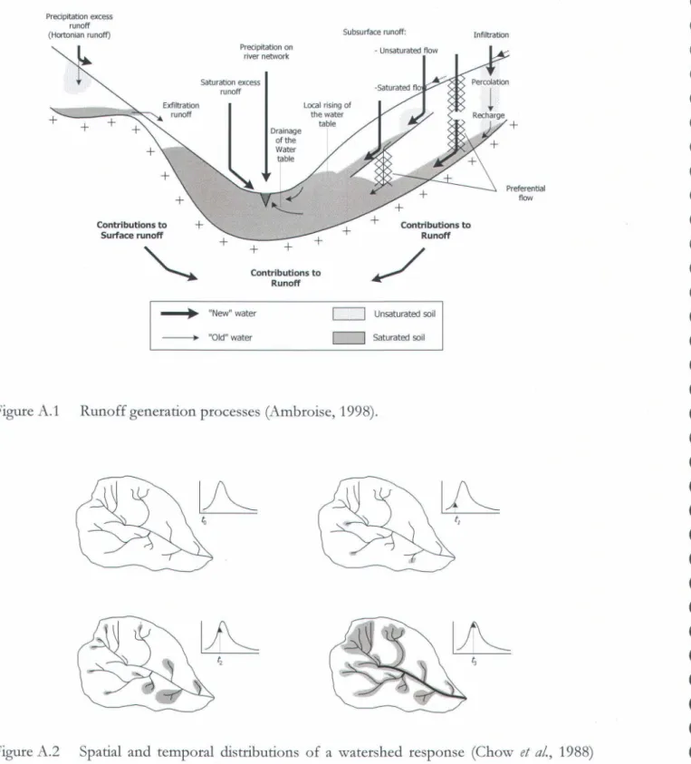
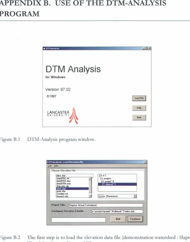
APPENDIX A. RUNOFF GENERATION PROCESSES ... 29
APPENDIX B. USE OF THE DTM-ANAL YSIS PROGRAM ... 31
APPENDIX C. PRESENTATION OF ROUSSEAU ET AL. MADE AT THE 2004 IROWCS HYDROLOGY TECHNICAL WORKSHOP HELD IN SAINTE-FOY, QUEBEC (FEBRUARY 18 AND 19) ... 35
•
•
•
•
•
•
•
•
•
•
•
•
•
•
•
•
•
•
•
•
•
•
•
•
•
•
•
•
•
•
•
•
•
•
•
•
•
•
•
•
•
•
•
•
•
•
•
•
•
•
•
•
•
•
•
•
•
•
•
•
•
•
•
•
•
•
•
•
•
•
•
•
•
•
•
•
•
•
•
•
•
•
•
•
•
•
•
•
Figure 2.1 Figure 2.2 Figure 2.3 Figure 3.1 Figure A.l Figure A.2 Figure B.l Figure B.2 Figure B.3 Figure B.4 Figure B.5 Figure B.6LIST OF FIGURES
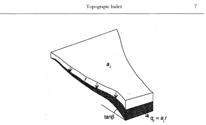
Illustration of the upslope area per unit contour length draining through a point i, ai [L], within a watershed. Where ris the recharge rate [LTi
]
over the upslope and qi is the subsurface flow per unit contour length
[L
or-
i] (Beven, 2001) ... 7 Spatial distribution of TI in a 3.8-ha watershed (Beven, 2001). High values of TI in valley bottoms and hillslope hollows imply that, in principle, these areas will saturate fIrst ... 7 Cumulative distribution function (CDF) and probability density function (PDF) in a 3.8-ha watershed (Beven, 2001) ... 8. Canadian areas covered by 1:250 000 and 1:50 000 CDED (GeoBase®) ... 12 Runoff generation processes (Ambroise, 1998) ... 30 Spatial and temporal distributions of a watershed response (Chow et al.,
1988) ... 30 DTM-Analysis program window ... 31 The fust step is to load the elevation data fIle (demonstration watershed: Slapton Wood Catchment, Devon, UK) ... 31 Once the elevation data fùe is loaded, the user has to choose between the three options ... : ... 32 Sink Removal Analysis Window ... 32 Catchment IdentifIcation Window ... : ... 33 TI Calculation window, with the elevation map (le ft) and the TI values map (right) ... 33
•
•
•
•
•
•
•
•
•
•
•
•
•
•
•
•
•
•
•
•
•
•
•
•
•
•
•
•
•
•
•
•
•
•
•
•
•
•
•
•
•
•
•
•
1 INTRODUCTION
To assess the risk or vulnerability of water contamination and identify critical parameters and management practices, Agriculture and Agri-Food Canada (AAFC) initiated, under the 1993 Agri-Environmental Indicator Project, the development of two Agri-Environmental Water Quality Indicators (AEWQIs) related to the potentialloss of soil phosphorus (P) and nitrogen (N). In 2001, under the National Agri-Environmental Health Analysis and Reporting Program (NAHARP), work was continued on the N and P Indicators of Risk of Water Contamination (IROWC) and development of a pesticides indicator and a pathogens indicator was undertaken. According to AAFC, the applications of IROWCs and their ensuing relations to economic and environmental models will improve and facilitate the decision making process needed to assess environmental policies in agriculture before they are put in place (Cessna and Junkins, 2003).
One of the databases used to derive IROWCs is the Census of Agriculture which covers ail agricultural regions of Canada. Agricultural production system characteristics such as cropland information, livestock numbers, soil properties, weather data, N and P fertilization practices are some of the data included in the Census. The other key database is the Canadian Soil Land Information System (CanSIS). This geographic database contains attributes of ail the distinct Soil Landscapes of Canada (SLC), that is, specific soil types and their corresponding characteristics (e.g., landform, slope, water table, permafrost, lakes). In the CanSIS database, SLCs are mapped using polygons, where a polygon is made up of the soil and land attributes of either: (i) one soillandscape with or without inclusions (that is, nonsoil features such as outcrops), (ü) two soillandscapes (the dominant and subdominant soillandscapes), or (fi) two soillandscapes and inclusions (Agriculture Canada, 1992). IROWCs may be calculated at the soillandscapes polygon level by linking, for example, the CanSIS database with the Census database. After either scaling up or down, these indicators may be aggregated at a regional or watershed scale. Values of IROWCs can be obtained from a weighted SUffi of intermediate values computed from specific algorithms or models
related to soil chemical balance, water balance, potential soil loss, soil water flows, etc.
Currently, some of the algorithms or models are firmly set while others are not. However, as reported at the 2004 IROWCs Hydrology Technical Workshop (Sainte-Foy, Quebec, February 18 and 19), the possibility of a common hydrology component for the four IROWCs should be investigated. Towards this, the Sainte-Foy Soils and Crops Research and Development Centre of AAFC mandated us to contribute to the development of the Hydr%gy Component of IROWC within the context of IROWC_P.
2 Integration of a Topographie Index in the Hydr%gy Component of IROWC_P
1.1 IMPORTANCE OF THE HYDROLOGY COMPONENT
Transport of pollutants from cropland to surface wate:rs depends on: (i) quantity and availability of soil agricultural chemicals, (ü) c:ropping practices and (fi) :rainfall-runoff processes. Fo:r P, studies have shown that runoff from soils with high degrees of P
saturation can contribute up to 40 % of the total river load, while anothe:r 40 % may come from soils with moderate degrees of P saturation but with high degrees of hyd:tological connectivity (i.e., proximity) to the rive:r netwo:rk (Schoumans and B:reeuwsma, 1997; Sha:rpley et al., 1999). Seve:ral studies have also shown that runoff from a :relatively small po:rtion of a wate:rshed (e.g., 10 % of the a:rea) , that located along the d:rainage/rive:r netwo:rk, may account fo:r all of the dissolved P load into a :rive:r (Gburek et al., 2000).
These fmdings show why hyd:tological p:rocesses need to be accounted fo:r in the development of IROWCs. Howeve:r, the :relationship between :rainfall and runoff is complex and influenced by many pa:ramete:rs such as geology, topog:raphy, soil cha:racteristics and land use. Thus, hyd:tological p:rocesses gove:rning runoff production have to be distinguished depending on these cha:racteristics. The th:ree hyd:rological p:rocesses gove:rning runoff a:re: p:recipitation/infùtration excess runoff (also :refe:r:red to as Ho:rtonian runoff), saturation excess runoff, and ex filtration runoff (see Appendix A).
1.2 ACCOUNTING FOR HYDROLOGICAL PROCESSES
Runoff processes at the agricultu:rallandscape level may be cha:racterized in diffe:rent ways by means of state variables, provided eithe:r by direct measurement, mathematical simulation using dete:rministic hyd:tologic models, o:r :rep:resentative indicato:rs.
Direct measurement of wate:r and pollutant balances provides a means of identifying the runoff processes :responsible fo:r wate:r contamination at va:rious scales, that is, f:rom the point scale th:rough the plot and hillslope scales (Quinn, 2002). Howeve:r, findings at these scales a:re difficult to scale up at the wate:rshed level because of the inc:reasing spatial and tempo:ral complexities of the runoff processes and inte:ractions between landscape, soil, and human activities.
Dete:rministic models a:re useful tools to simulate complex and multi-factorial processes on the basis of cu:r:rent scientific knowledge. In the case of environmental risk assessment, sorne integrated models, such as SWAT (Neitsch et al., 2000) o:r GIBSI (Mailhot et al., 1997; Rousseau et al., 2000, 2002; Villeneuve et al., 1998), provide a means of evaluating the effects of ag:ricultu:ral management scena:rios on wate:r quantity and quality at the wate:rshed scale,
•
•
•
•
•
•
•
•
•
•
•
•
•
•
•
•
•
•
•
•
•
•
•
•
•
•
•
•
•
•
•
•
•
•
•
•
•
•
•
•
•
•
•
•
•
•
•
•
•
•
•
•
•
•
•
•
•
•
•
•
•
•
•
•
•
•
•
•
•
•
•
•
•
•
•
•
•
•
•
•
•
•
•
•
•
•
•
•
Introduction 3for instance. However, such models requtte extensive input data (i.e., variables and parameters related to soils characteristics, topography, river network, land use, cropping practices, and meteoralogical variables, etc.) that make their use complex.
As an alternative, indicators represent a compromise when compared to data derived from deterministic models. The purpose of indicators is to simplify a complex system so as to make the reality accessible to users in the form of diagnostic or decision support tools/indices (Girardin et al., 1999). Indicators must be easily quantifiable and quickly reveal changes of states. Values taken by an indicator are not usable in an absolute sense, but are of interest with respect to a spatial or temporal frame of reference.
1.3 THE PROPOSED APPROACH: A TOPOGRAPHIC INDEX
For areas with gende slope and shallow soils on an impermeable rock or impervious soil layer, topography plays a key raIe in surface runoff production, especially under temperate and humid climate conditions where saturation excess runoff dominates (see Appendix A). For these areas, and under these specific conditions, Beven (2001) reports that the surface runoff pracess can be predicted with an index of hydrological similarity based on topographic considerations [ex: the Kirkby index, base of the TOPMODEL hydrological model of Beven etaI. (1995)].Following this concept, all topographic units or spatial elements of a watershed with an identical index value develop, in princip le, the same conditions for saturation, surface and subsurface flow / runoff. In the context of a soil rich in nutrients, pesticides or pathogens, and suitable to the production of saturation excess runoff, the knowledge of topographic index values can be used to illustrate the spatial distribution of watershed areas with a risk of pollutant loss from soil to surface waters, that is the "hydrologically" connected areas. For N and P, Quinn (2002) refers to the terms critical source areas (CSAs) and variable source areas (VSAs) to describe water contamination by surface source areas and subsurface source areas, respectively. VSAs are generally topographically controlled while CSAs are controlled through management practices.
The goal of this study is to assess the feasibility of integrating a topographic index (TI) of hydrological similarity in the Hydr%gy Component of IROWC_P. Specifically, the scope of this report is to present:
(i) the rationale behind the use of TI; that is defmition, conditions of application and determination;
4
(ü)
Integration of a Topographie Index in the Hydralogy Component of IROWC_P
the availability of data and algorithms required to apply and detetmine TI values at the nationallevel; and
(iü) the potential integration of TI in the Hydr%gy Component of IROWC.
Note that an initial assessment of the feasibility of integrating TI in the aforementioned Hydr%gy Component was presented at the 2004 IROWCs Hydrology Technical Workshop
(see Appendix C).
•
•
•
•
•
•
•
•
•
•
•
•
•
•
•
•
•
•
•
•
•
•
•
•
•
•
•
•
•
•
•
•
•
•
•
•
•
•
•
•
•
•
•
•
•
•
•
•
•
•
•
•
•
•
•
•
•
•
•
•
•
•
•
•
•
•
•
•
•
•
•
•
•
•
•
•
•
•
•
•
•
•
•
•
•
•
•
•
2 THE TOPOGRAPHIe INDEX (TI)
Hydrological processes are dynamically and heterogeneously distributed in space and cime. Furthermore, interactions between landscape, soil and rainstorm dynamics make the runoff phenomenon difficult to predict and model (Beven, 2001). However, the topographic control of surface and subsurface flows may be suitable to a macroscale conceptualization of the rainfall-runoff process (Beven, 2001). For the case of a shallow soil relative to a hillslope scale, this gravitational pattern can lead to a water table that is nearly parallel to the topography over much of the hillslope length. This is particularly true if there is a constant recharge rate over the hillslope and if the surface slope is equal to the local downslope hydraulic gradient. U nder these conditions, water is expected to flow downhill from steep to shallow slope, and into areas of slope convergence.
In any watershed, there may be many areas that behave in a "hydrologically" similar fashion, with similar water balance and runoff generation characteristics, whether by surface or subsurface flow. If it were possible to classify areas or points within a watershed in terms of their hydrological similarity, then a hydrological model could be developed based on hydrogeomorphological aspects of runoff formation, without the requirement of considering all individual areas independently (Beven, 2001). The TOPMODEL of Beven et al. (1995) is based on this premise; that is the distributed predictions of watershed responses are made based on a simple theory of hydrological similarity of points within the watershed.
Although this report refers to TOPMODEL (Beven et al., 1995), it is not the intent here to further elaborate on this hydrological model since the primary focus is on the TI concept. Nonetheless, when the report introduces elements of discussion pertaining to TOPMODEL, it does so to enrich the presentation without loss of continuity and as a means of illustrating how the TI concept has been used in a hydrological modeling context.
2.1 HYDROLOGICAL SIMILARITY: THE TI CONCEPT
The hydrologic similarity concept is based on two assumptions:(1) the dynamics of the saturated zone may be viewed as successive steady-states of the saturated zone on an area ai draining to a point i on a hillslope; and
(ii) the hydraulic gradient of the saturated zone can be approximated by the local surface topographic slope measured with respect to plan angle tan(f3J.
6 Integration of a Topographie Index in the Hydrology Component of IROWC_P
In tenus of hydrological modeling, these assumptions lead to a simple relationship between watershed storage (or storage deficit below saturation) in which the main factor is the Kirkby topographic index (Kirkby 1975; Beven 2001) also referred to as TI:
TI=1n(
ai )1 tan([Ji)
(2.1)
TI
i represents the propensity of a point i in a watershed to develop saturated conditions and,hence, contribute to saturation excess runoff. High values will be caused by either long slope or upslope contour convergence and low slope angles, and the corresponding areas will tend to saturate first. Thus, these points delineate potential surface or subsurface contributing areas to watershed runoff (i.e., VSAs).
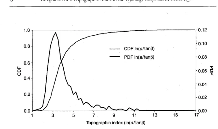
Figures 2.2 and 2.3 depict the spatial and statistical distributions of
TI
values on a studied watershed, where, without loss of continuity, the index i was dropped. As pointed out by D'Odorico and Rigon (2003), it is possible to estimate the probability distribution of TI andfor any value of a quantile,Q, to map the corresponding VSAs having a TI value of v(Q). P[TI ~
v(Q)]
=
Q
(2.2) From a hydrogeomorphological point of view, this mapping allows for the identification of the "hydrologically" connected parts of the watershed given a fixed value of the quantile.As mentioned earlier, the TI approach was developed into a complete rainfall-runoff model,
TOPMODEL (Beven and Kirkby, 1979; Beven et al., 1995), and generalized to allow for differences in soil characteristics within a watershed. Within this context, the use of the Kirby index is based on a third assumption:
(iii) the distribution of the downslope transmissivity with depth can be represented by an exponential function of storage deficit or depth to the water table:
T =T -D/m
II (2.3)
Where Ta is the horizontal transmissivity when the soil is saturated (expressed in [I}y-l]), and D is a local storage deficit below saturation expressed as a water depth [L] and m is a model parameter which control the rate of de cline of transmissivity in soil profùe (expressed in [L]).
•
•
•
•
•
•
•
•
•
•
•
•
•
•
•
•
•
•
•
•
•
•
•
•
•
•
•
•
•
•
•
•
•
•
•
•
•
•
•
•
•
•
•
•
•
•
•
•
•
•
•
•
•
•
•
•
•
•
•
•
•
•
•
•
•
•
•
•
•
•
•
•
•
•
•
•
•
•
•
•
•
•
•
•
•
•
•
•
T opograpic Index 7Figure 2.1 Illustration of the upslope area per unit contour length draining through a point i, ai [L], within a watershed. Where ris the recharge rate [LTi] ove! the upslope and
q)s the subsurface flow per unit contour length [L zr-i] (Beven, 2001).
ln (a/ tanf3J
270
250
Figure 2.2 Spatial distribution of TI in a 3.8-ha watershed (Beven, 2001). High values of TI in valley bottoms and hillslope hollows imply that, in principle, these areas will saturate fttst.
8 1.0 0.8 0.6 LL. 0 ü 0.4 0.2 0.0 1
Integration of a Topographie Index in the Hydrology Component of IROWC_P
3 5 7 9
CDF ln(altan~)
PDF In(a/tan~)
11 13
Topographie index (ln(a/tan~)
15 0.12 0.10 0.08 "U 0.06 Cl "Tl 0.04 0.02 0.00 17
Figure 2.3 Cumulative distribution function (CDF) and probability density function (PDF) in a 3.8-ha watershed (Beven, 2001).
2.2
APPLICATION CONDITIONS AND LIMITATIONS
In the context of various TOPMODEL applications, Beven et al. (1995) and Beven (2001) reviewed the evidence for the success of the TI concept in predicting patterns of saturation (i.e., soil moisture and water table depths) in different field/modeling studies. Sometimes the saturation patterns appear adequate, sometimes they do not. These inconstancies can be best explained by examining the way the TI concept simplifies the dynamics of a watershed and by underlining the fact that the underlying assumptions may occasionally be too strict. Note that Beven (1997) has published a complete critique ofTOPMODEL.
The first assumption, wruch views the dynamics of the saturated zone as successive steady-states, implies that there are a constant recharge rate and a downslope flow everywhere over the hillslope wruch is clearly not the case where hillslopes are seasonally dry. Indeed under these conditions (e.g., Beven, 1997, 2001; Blazkova et al., 2002): (i) the effective upslope
contributing areas do not extend to the hillslope divide or boundary, and (ü) the saturated zone may become localized and isolated so the effective TI value reduces, only to re-expand during wetting as the contributing areas spread. From a modeling point of view, this behavior leads to a difficulty in estimating subsurface flow dis charge during wetting-up periods. Discharge rates can be spatially and dynamically non-uniform since they temporally change during a storm event or dry spell so steady state conditions are never actually met. Beven and Freer (2001)
•
•
•
•
•
•
•
•
•
•
•
•
•
•
•
•
•
•
•
•
•
•
•
•
•
•
•
•
•
•
•
•
•
•
•
•
•
•
•
•
•
•
•
•
•
•
•
•
•
•
•
•
•
•
•
•
•
•
•
•
•
•
•
•
•
•
•
•
•
•
•
•
•
•
•
•
•
•
•
•
•
•
•
•
•
•
•
•
Topograpic Index 9established that under such conditions, the development of a perched water table would limit the validity of any index-based approach. Hence, in watersheds where there is a long dry season and a long wetting up period, the dynamics or lack of steady-state saturated flow conditions will, on one hand, restrict the use of TOPMODEL, and on the other hand, highlight the fact that the dynamics of the contributing areas are governing the hydrological behavior of the watershed.
There are also concerns about the second assumption where the premise is that the water table is nearly parailel to surface topography for relatively thin soils over an impermeable soillayer on moderate slopes. Under this condition, the hydraulic gradient is assumed to be equal to the slope angle. However, this behavior will be violated as soils get deeper or if there is a strong spatial or temporal change in the recharge rate (Beven and Freer, 2001). Many local effects on groundwater may also lead to variations of the second assumption pattern as weil (e.g.,
existence of substantial preferential flows).
Given the above observations, TOPMODEL should not be expected to perform weil on ail watersheds. However, the model willlikely perform weil when applied on watersheds where ail the underlying conditions are met, particularly those related to the first two assumptions, that is, those of a topographic control of the water table depth and a quasi-parailel water table with respect to hillslope topography. From a lands cape point of view, these watersheds are likely to have relatively shailow, homogeneous, soils where surface and subsurface flows are governed by contributing areas exhibiting saturation excess runoff. On the other hand, on watersheds where precipitation/infiltration excess runoff processes are thought to be important, it is unlikely that the assumption of a topographicaily controiled water table holds. These restrictions or constraints do not invalidate the TI concept but rather highlight the circumstances or conditions under which TOPMODEL should be applied and the need to extend the concept to other conditions (see Ambroise et al., 1996a,b).
2.3 COMPUTATION OF TI
As mentioned by Beven et al. (1995) and Beven (2001), in the early stage of development of TOPMODEL, computation of TI relied upon manual analysis (based on map and air photo information) of local slope angles, upslope contributing areas and cumulative areas. Nevertheless, Beven and Kirkby (1979) proposed a computerized technique to derive the TI
distribution function based on the division of the watershed into smail "local" slope elements on the basis of dominant flow paths identified with field observations. Flow paths were inferred from lines of greatest slopes and computation of TI was performed for the downslope edge of each element. This technique was particularly useful to delineate the effects of
man-10 Integration of a Topographie Index in the Hydrology Component of IROWC~P
made infrastructures, such as field drains and roads, m controlling effective upslope contributing areas.
Digital Terrain Analysis (OTA) programs, based on raster elevation data, are now available to derive the required topographic information by TOPMODEL. Applications of these programs to watershed studies have been described by Quinn et al. (1991) and Quinn and Beven (1993). The availability and description of these programs are introduced in Chapter 3. The Eunctional nature of TI depends on the quality of the representation of hydrologicaily significant topographic features by DTA methods.
To derive TI, a scale of resolution for the watershed DTM must first be selected. The DTM must have a fme enough resolution to properly reflect the effect of topography on surface and subsurface pathways (O'Odorico and Rigon, 2003). Coarse resolution DTMs may fail to represent sorne convergent slope features and sorne apparent sources or sinks for water contaminants. However, too fine a resolution may introduce perturbation to flow directions and slope angles that may not be reflected in the smoother water table surface (Quinn,2002). The appropriate resolution depends on the scale of the hillslope features, but 50 m or better data is normaily suggested (Beven, 2001).
2.4 SUMMARY
From an indicator point of view, the TI concept should be used to predict the propensity of a point in a watershed to develop saturated conditions and, hence, contribute to saturation excess runoff. For a soil rich in potential water contaminants and likely to be the site of saturation excess runoff, knowledge of TI values will clearly illustrate the spatial distribution of watershed areas with a high risk of poilutant loss to surface waters.
It is noteworthy that most Canadian prairies watersheds do not have shailow soil systems, with moderate slope angle, and a long wet season. In fact, most of the prairies have relatively deep soils and are exposed to a long dry season where perhaps infiltration excess runoff might dominate the runoff production process during the summer. This said, we believe the TI
approach can be used with confidence as an indicator of saturation excess runoff where it applies, that is, in eastem Canada and on the Canadian west coast where the upslope contributing area generaily extends to the hillslope divide during fail, winter and spring. For summer and for the Canadian prairies, the use of TI as an indicator of water contamination by agricultural nutrients should be used with care as it is more likely that the Hortoruan runoff process dominates. Nevertheless, we firmly believe that it will be useful to determine TI values for those watersheds and conditions.
•
•
•
•
•
•
•
•
•
•
•
•
•
•
•
•
•
•
•
•
•
•
•
•
•
•
•
•
•
•
•
•
•
•
•
•
•
•
•
•
•
•
•
•
•
•
•
•
•
•
•
•
•
•
•
•
•
•
•
•
•
•
•
•
•
•
•
•
•
•
•
•
•
•
•
•
•
•
•
•
•
•
•
:
.
•
•
•
•
•
3 AVAILABILITY OF
DATA AND
ALGORITHMS
To de termine TI values at the scale of Canadian agricultural areas, the following data and algorithms are required:
(i) digital elevation data with a fine grid resolution (50 m or better, if possible) and
(ü) software or algorithms to calcula te the ln (a/ tan/3) spatial distribution based on the digital elevation data
3.1 AVAILABILITY OF DIGI
T
AL ELEVATION DATA AT THE
CANADIAN SCALE
Canadian Digital Elevation Data (CDED) are produced jointly by the Centre for Topographical Information (CTI) and the Canadian Forest Service, Ontario Region (CFS).
These data are free of charge and readily available on the GeoBase website
(http://www.geobase.ca/geobase/Geobase).
CDED consist of an ordered array of ground elevations at regularly spaced intervals. They are derived &om the National Topographic Data Base (NTDB) digital files at the 1:50000 and 1:250000 scales, based on the divisions of the National Topographic System (NTS). All CDED fùes are produced using ANUDEM (Australian National University Digital Elevation Models) software, after scanning NTS map sheets. An important distinguishing feature of the
ANUDEM approach is the fact that it includes the identification and correction of mislabelled contour data and provides a properly flowing connected streamline hydrology.
The number of points per profile and the number of profiles per cell are constant for all the files (1201 x 1201). Each cell holds 1 442401 elevation points. The North American Datum of 1983 (NAD83) is used as the reference system. Elevations are orthometric and expressed in reference to the Mean Sea Level (Canadian Vertical Geodetic Datum).
The grid spacing of the CDED is based on geographic coordinates. Cell coverage varies according to three geographic areas: below the 68th parallel, between the 68th and the 80th parallel, and beyond the 80th parallel (Centre for Topographic Information, 2000). As
agricultural regions are located in the first area, this report focuses on this are a and ignores the
12 Integration of a Topographie Index in the Hydrology Component of IROWC_P
For 1:50000 CDED, the ceil coverage is 15' x 15' with a grid spacing of 0.75" x 0.75", wruch
corresponds to approximately 23 m (N-S) x 16-11 m (E-W, depending upon latitude). For
1:250000 CDED, the ceil coverage is 10
x 10
with a grid spacing of 3" x 3", wruch
corresponds to approximately 93 m (N-S) x 65-35 m (E-W, depending upon latitude).
Note that Digital Elevation Model (DEJ\II) at coarser scales have been produced by the Landscape Analysis and Applications Section (LAAS) at the Canaruan Forest Service, based 9n
a resampling of the 1 :250 000 DEM.
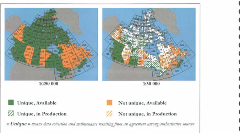
3.1.1 Territory Coverage
The 1:250000 CDED provides complete seamless coverage of the encire country (see Figure 3.1). Most of the 1:50000 CDEDs are currently in production (no publication date is available from GeoBase). They will only provide a partial coverage of the country, mainly in inhabited
areas and where economic activity is significant. At present, only British Columbia, Southern
Saskatchewan and a large part of the Maritime Provinces are covered (see Figure 3.1).
1:250000 1:50000
• Unique, Available • Not unique, Available
~ Unique, in Production ~ Not unique, in Production
« Unique» means data collection and maintenance resultingfrom an agreement among authoritative sources
Figure 3.1 Canaruan areas covered by 1:250000 and 1:50 000 CDED (GeoBase®)
•
•
•
•
•
•
•
•
•
•
•
•
•
•
•
•
•
•
•
•
•
•
•
•
•
•
•
•
•
•
•
•
•
•
•
•
•
•
•
•
•
•
•
•
•
•
•
•
•
•
•
•
•
•
•
•
•
•
•
•
•
•
•
•
•
•
•
•
•
•
•
•
•
•
•
•
•
•
•
•
•
•
•
•
•
•
•
•
Availability of Data and Algorithms 13
As previously indicated, the suggested grid resolution for determination of TI is 50 m or better, fmer resolution being better. Therefore, 1:50000 CDED will be used where available, and 1:250000 CDED will be used elsewhere (see Figure 3.1).
3.1.2 File Format
The fùe format is very similar to the ASCII version of DTED of the United States Geological Survey (USGS). Therefore, the data are compatible with ail translators designed for the USGS DTED.
3.2 AVAILABILITY OF ALGORITHMS
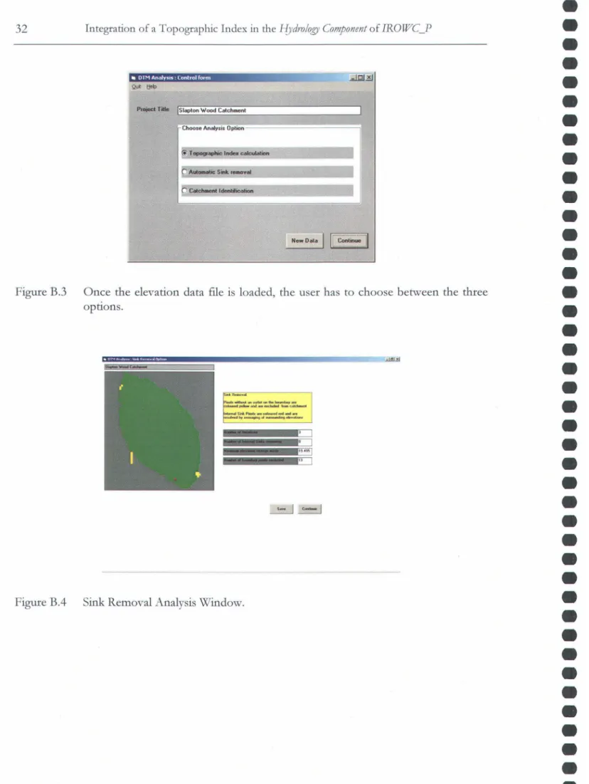
Several programs are readily available, free of charge, on TOPMODEL website (http:/h'v'\v'w.es.lancs.ac.uk/hfdg/beven2000/Beven2000.html): TOPMODEL, TFM, GLUE and DTM-ANALYSIS.
The program of interest here is the DTM-ANALYSIS program, which contains three options (see Appendix B for a description of the software). The TI Distribution Calculation option enables the derivation of a distribution of In(a/tan,8) values from a regular raster grid of elevations for any watershed or subwatershed. The calculation algorithm is based on the multiple direction flow algorithm of Quinn et al. (1995). The output is a histogram of the distribution of the In(a/tan,8) values, and a map file of In(a/tan,8) values. However, the simple use of this algorithm with an elevation data grid may lead to high TI values for pits and sinks which are not connected to river network. To avoid these misleading results, the Automatic Sink Removal option ailows for the modification of the elevation data and removal of sinks by using successive averaging of surrounding elevations to resolve pits. Additionaily, this feature handles the case of smail river channels for which the elevation grid cannot resolve the continuous flow pathway. The TI Distribution Calculation also requires that only elevations of points within the watershed are supplied, ail other values in the matrix being set to greater than a value of 9999.0 (m). The Catchment Identification option provides for values above a specified pixel value to be removed from the watershed using a hill climbing algorithm. This option is important in the current context since the elevation data that will be used do not have watershed boundaries a priori.
As previously mentioned, it is recommended that the elevation data should be at a 50 m resolution or better. It should be noted that the derived In(a/tan,8) distribution will be dependent on the resolution of the elevation data used and on the particular rules for
14 Integration of a Topographie Index in the Hydr%gy Component of IROWC_P
distributing upslope areas and dealing with river channels that are smailer than the grid size. Different distributions may result in different effective parame ter values for a given watershed.
3.2.1 Input File Format
Only one flle is required to mn the program. This is a file of elevations in metres, listed in order from the bottom left hand (south west) corner of the map, row by row working northwards. The fttst line of the file must contain an 80 character tide; the second line the number of columns, the number of rows and the grid spacing in m. It is assumed that ail points falling outside of the watershed have already been identifled and given an elevation >
9999. The input elevation file should thus have the foilowing form:
1. Tide Descriptive tide for watershed or elevation grid 2. NX,NY,DX Number of columns, number of rows, grid size (m) 3. ((E(I,J),I=l,NX),J=l,NY) Elevation values ordered row by row
3.2.2 Output Files
Two flles are produced by the DTM-ANALYSIS program, formatted to be direcdy used in TOPMODEL program:
(i) An ASCII flle with the distribution of the ln(a/tan,8) values. Values are classifled into 50 classes, and the flle gives the frequency and the cumulative frequency corresponding to each class. These data enable to do statistical analyses.
(ü) An ASCII file with ln(a/tan,8) values, foilowing the same structure as input file with elevation data:
1. Tide Descriptive tide for watershed or elevation grid 2. NX,NY,DX Number of columns, number of rows, grid size (m) 3. ((T(I,J),I=l,Nx),J=l,NY) ; Topographie index values ordered row by row This flle can be used to visualize spatial distribution of topographie index values with any Geographie Information System (GIS) software, after transformation of the ASCII file into a raster file format by the mean of importation tools.
•
•
•
•
•
•
•
•
•
•
•
•
•
•
•
•
•
•
•
•
•
•
•
•
•
•
•
•
•
•
•
•
•
•
•
•
•
•
•
•
•
•
•
•
•
•
•
•
•
•
•
•
•
•
•
•
•
•
•
•
•
•
•
•
•
•
•
•
•
•
•
•
•
•
•
•
•
•
•
•
•
•
•
•
•
•
•
•
Availability of Data and Algorithms 15
3.2.3 File Format Compatibility
The file format of CD ED cannot be direcrly used as input flle for DTM -ANAL YSIS program. A simple adaptation algorithm will be required to convert the CDED files to a compatible format. Another problem is the grid ceil dimension: in the CDED, the ceillength and width are not equal, while a square ceil size is required in DTM-ANALYSIS program. To resolve this issue, a simple geomatic procedure (i.e. a Lambert conic projection) will be used.
3.3 SUMMARY
This Chapter introduced the relevant data and algorithm/program/software needed to compute TI values at the scale of Canadian agricultural areas. Namely, the required DTMs can be obtained, free of charge, from CDED at either a 1:50000 or 1:250000 scale. While the required DTM-ANALYSIS program can be downloaded from the TOPMODEL website.
•
•
•
•
•
•
•
•
•
•
•
•
•
•
•
•
•
•
•
•
•
•
•
•
•
•
•
•
•
•
•
•
•
•
•
•
•
•
•
•
•
•
•
•
•
•
•
•
•
•
•
•
•
•
•
•
•
•
•
•
•
•
•
•
•
•
•
•
•
•
•
•
•
•
•
•
•
•
•
•
•
•
•
•
•
•
•
•
4 INTEGRATION OF TI IN THE HYDROLOGY
COMPONENT OF IROWC
In this Chapter, the integration of TI is analysed and proposed in terms of IRO WC_P. Also, as mentioned in the fust chapter, we explore means of integrating the representation of the TI concept at the SLC polygon, that is, the elementary unit of the IROWC computational domain.
4.1 PROPOSED METHOD
The calculation of IROWC_P was initiaily defmed as foilows:
IROWC _ P
=
P _ Balance+
P _ 5tatus+
P _ Transport (4.1) This formulation corresponds to the Phosphorus Index (PI) introduced by (Lemunyon and Gilbert, 1993). The P _Transport Component (or Hydrology Componenf) consists of the addition of two terms: P _Runriff and P _Erosion. The P _Runriff term is a runoff index calculated using the SCS-Curve Number method (USDA, 1972). The P _Erosion term is an erosion index calculated with the RUSLE model (pringle et al., 1995). Moreover, ail components are weighted by a rating value, different for each studied area, and a weighting factor that has to be adjusted for each indicator.4.1.1 Integration of TI in the Hydrology Component
First of ail, we propose to combine the 50il Component (P _Balance
+
P _5 tatus) and the Hydrology Component since they are independent and limiting factors for poilutant loss from soils to surface waters as foilows:IRO WC _ P
=
(P _ Balance+
P _ 5 tatus) X P _ Hydrology (4.2) With this formulation, an area with a high P content but without any hydrological connectivity would have an IRO WC_P value of O.18 . Integration of a Topographie Index in the Hydr%gy Component of IROWC_P
4.1.2 Hydrology Component Formulation
Several other eomponents are in the process of being added to those already in place: Water Balance, Sutjace Drainage, Subsutjace Drainage, and TI. These components should be considered in an additive way since most of them are somewhat dependent or intrinsicaily related.
An important issue is to avoid any overlap between the different terms, and this is especiaily worth investigating in the case of the TI term, the P _Runrff term, and the Water Balance term since they are ail meant to deal with ronoff processes. The SCS-CN method used to calculate the P _Runrff term is rooted in a conceptual model based on the water balance equation and represents a hydrological abstraction of the Hortonian or excess infùtration ronoff process (see Chapter 1 and Appendix A) during a rainstorm event. The ronoff volume depends on rainfail intensity, initial soil moisture conditions, and land use. On the other hand, TI is an indicator of the propensity of a watershed area for saturation excess ronoff, and thus has nothing to do with Hortonian ronoff. Therefore, these two terms are meant for different processes, at different spatial and temporal scales, and can be used in a complementary way within the
Hydrology Component. Another difference is that TI accounts for neither precipitation nor water balance, while the SCS-CN method does. That is why it is also important to introduce a Water Balance term, calculated on a daily time-step; that ailows for the estimation of the annual volume of water available for saturation excess ronoff and/or infiltration. Note that there is a potentialoverlap between the P _Runrffterm and the Water_Balance term; an issue that will need to be addressed.
The proposed formulation of the Hydrology Component is as foilows:
Hydrology= P _Runrff+ P _Erosion
+
Water _Balance+ TI+
5 utjace_Drainage+ 5 ubsutjace_Drainage (4.3) The objective of the Hydrology Component formulation is to reproduce the main processes that are involved in contaminant transport from soils to surface waters and the water table. In this formulation, the two fttst terms (P-Runrff and P-Erosion) represent storm event processes producing excess infùtration ronoff (i.e., Hortonian ronoff). The terms Water Balance and TIaccount for the propensity of producing ronoff and saturation excess ronoff, respectively. The two last terms (Sutjace Drainage and Subsutjace Drainage) represent the artificial hydrological connectivity to surface waters and the water table. Note that TI indirecdy accounts for the natural (akin to floodplains) hydrological connectivity to surface waters and the water table.
•
•
•
•
•
•
•
•
•
•
•
•
•
•
•
•
•
•
•
•
•
•
•
•
•
•
•
•
•
•
•
•
•
•
•
•
•
•
•
•
•
•
•
•
•
•
•
•
•
•
•
•
•
•
•
•
•
•
•
•
•
•
•
•
•
•
•
•
•
•
•
•
•
•
•
•
•
•
•
•
•
•
•
•
•
•
•
•
Integration of TI in the Hydr%gy Component 19 Obviously, all these terms do not have the same relative importance with respect to each pollutant considered in the development of IROWCs. The weighting values that are attributed to each term, will take different values for different IROWCs, and, thus, the selection of the most important factors and processes with that respect. Finally, other terms could be added to improve the overall representation of the hydrological processes responsible for water contamination (i.e., macropore or preferential flow), but that is beyond the scope of this study.
4.2 SEASONAL PARTITIONING
One way to avoid any overlap and to take advantage of the complements of the different terms of the Hydrological Component would be to consider a seasonal partitioning in the calculation of
IROWC_P. For example, under Canadian conditions, a large part of the annual P load in surface waters occurs during the spring season. Since a large part of the P transport process is governed by saturation excess runoff due to snowmelt, the terms Water Balance and TI become the most important driving factors for delineating the areas with a high risk of water contamination during this period. A similar assumption can be made for the fall season since the contributing areas are mainly those defmed by TI.
Meanwhile, during summer, the principal hydrological processes responsible for P transport from soils to surface waters are likely to be induced by precipitation excess runoff. Therefore, for a better assessment of the P contributing areas, the P _Erosion and P _Runiff terms should be considered as the dominant terms of the Hydrology Component during this period.
This seasonal partitioning could be achieved by assigning a different weighting value for each season, and by calculating the terms that depend on climatic factors (Water Balance, P _Runiff
and P _Erosion) on a seasonal rime step, instead of determining an annual average value.
4.3 TI VALUE AT SLC POLYGON LEVEL: COMPATIBILITY
ISSUES
The elements of the spatial compatibility issues are related to the following observations:
(i) The elevation data that is required to calculate TI are available at a scale of 1 :50 000 or 1:250000 with grid cells containing 1201 x 1201 elevation points (or pixels). This corresponds to a coverage of 27,6 km (S-N) x 19,2 km (E-W) for the 1 :50 000 CDED, and 111,6 km (S-N) x 82,8 km (E-W) for 1:250000 CDED, for low latitude regions.
20
(ü)
Integration of a Topographie Index in the Hydrology Component of IROWC_P
The DTM-ANALYSIS program can be used to define watershed delimitations based on elevation data and calculate TI values for each pixel of a watershed.
(iü) The determination of a single value of TI at the scale of each SLC polygon (a scale of 1:1 000000. The size of a SLC polygon may vary in a wide range (100 km2 to 10000 km2
).
There are three information layers that need to be considered: polygons, watersheds, and elevation data grid ceils. The use of a GIS software will enable the superimposition of these layers and the management of the data. As these three spatial scales are independent, it is necessary to de termine TI values for each pixel contained within a polygon in order to de termine a single value for the whole polygon. So we need to determine the TI values for ail the watersheds that have a connection with a SLC polygon. To do so, ail watersheds have to be identified by the DTM- ANALYSIS program, and which requires running the program, not on each grid ceil separately, but on an aggregated grid ceil containing ail the elevation data of the watersheds that are connected to the SLC polygon.
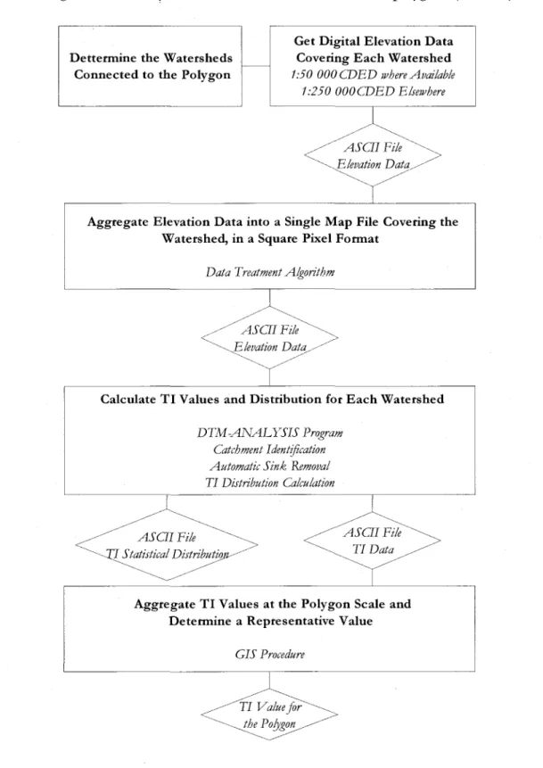
Therefore, we first have to defme a range of size for the watersheds on which TI will be determined separately. As we will mainly use 1:250000 CDED (see Section 3.1), and as the covered area for a single CDED is around 9000 km2
, it seems more appropriate to consider large watersheds. The foilowing procedure will have to be applied for each watershed (see Figure 4.1): the first step is to identify the grid ceils of CDED that contain a part of the watershed. This can easily be done with a GIS. The second step requires the aggregation of the elevation data of each CDED grid ceil to a single grid ceil covering the whole watershed. This task can also be performed with a GIS, but only if ail the CDEDs are at the same scale (1:50000 or 1:250000). The third step consists in running the DTM-ANALYSIS program to identify the watershed delimitations with the Catchment Identification option, to remove sinks and pits with the Automatic Sink Removal option and then run the TI Distribution Calculation algorithm. This will generate a TI value for each pixel contained in the watershed.
Once ail the watersheds that are contained in - or connected to - the polygon of interest (in the case of a smail polygon, it may also be contained in a single watershed), a simple GIS procedure will ailow for the generation of a map file with a TI value for each pixel contained in the polygon. Finaily, the last step consists of choosing a statistical value that will represent the whole polygon in the Hydr%gy Component. the mean, the median, the mode? As the typical
distribution of TI values is strongly asymmetric with numerous low values and few high values, it is important to choose a statistical indicator that represents ail the values and especiaily the extreme values. Therefore, the mean value is the more appropriate statistical moment. However, to consider high risk water contamination conditions, it is also possible to calculate
•
•
•
•
•
•
•
•
•
•
•
•
•
•
•
•
•
•
•
•
•
•
•
•
•
•
•
•
•
•
•
•
•
•
•
•
•
•
•
•
•
•
•
•
•
•
•
•
•
•
•
•
•
•
•
•
•
•
•
•
•
•
•
•
•
•
•
•
•
•
•
•
•
•
•
•
•
•
•
•
•
•
•
•
•
•
•
•
Integration of TI in the Hydrology Component 21
other quartile values. Note that the size of the watersheds used for TI calculation may be reduced for regions covered by 1:50 000 CDED and for small SLC polygons (100 km2
).
Dettermine the Watersheds Connected to the Polygon
Get Digital Elevation Data Covering Each Watershed
1:50 000 CDED where Available 1 :250 OOOCDED Eisewhere
ASCII File Elevation Data
Aggregate Elevation Data into a Single Map File Covering the Watershed, in a Square Pixel Format
Data Treatment Aigorithm
ASCII File Elevation Data
Calculate TI Values and Distribution for Each Watershed
ASCII File
DTM-ANALYSIS Program Catchment Identification Automatic Sink fumoval TI Distribution Calculation
l Statistù-al Distributio
ASCII File TI Data
Aggregate TI Values at the Polygon Scale and Determine a Representative Value
GIS Procedure
TI Valuefor the Polygon
22 Integration of a Topographie Index in the Hydrology Component of IROWC_P
4.4 SUMMARY
This ehapter discussed the potential integration of TI in the Hydrology Component of IROWCs.
We proposed to consider TI as an additive factor together with (in the case of P) : Runriff, P-Erosion, Suiface Drainage, Subsuiface Drainage, and Water Balance terms. The result shail be
multiplied by the numerical value of the Soil Component (P _Balance
+
P _Status) to obtain IROWC_P. AIso, we proposed to take into account a seasonal partitioning in the Hydrology Component in order to improve the differentiation between saturation excess runoff (spring, fail)from infùtration excess runoff (summer). Finaily, a protocol was put forward for the up- or down-scaling of TI at the SLC polygon level, by ftrst aggregating elevation data (CDED) into a
single fùe for each watershed connected to the polygon, running the DTM-ANALYSIS program on this data @e, and then use a GIS procedure to get a spatial distribution of TI
values at the polygon level, which ailows for inferring a single representative value.
•
•
•
•
•
•
•
•
•
•
•
•
•
•
•
•
•
•
•
•
•
•
•
•
•
•
•
•
•
•
•
•
•
•
•
•
•
•
•
•
•
•
•
•
•
•
•
•
•
•
•
•
•
•
•
•
•
•
•
•
•
•
•
•
•
•
•
•
•
•
•
•
•
•
•
•
•
•
•
•
•
•
•
•
•
•
•
•
5 CONCLUSION
The topographic index (Tl) of hydrological similarity of Kirby (Kirby, 1975; Beven, 2001) has been used to represent the propensity of any point i in a watershed to develop saturated conditions and, hence, contribute to saturation excess runoff. High values of TI, defmed by the naturallogarithm of the ratio of the upslope draining area at that point over the local slope, are representative of either long slope or upslope contour convergence and low slope angles. These corresponding areas will tend to saturate fust. For a soil rich in nutrients, pesticides or pathogens, and suitable to the production of saturation excess runoff, the knowledge of TI
values can be used to illustrate the spatial distribution of watershed areas with a risk of water contamination (i.e., VSAs). The goal of this study was to assess the feasibility of integrating a
TI term within the Hydrology Component of IRO WC_P. With this respect and more specificaily in terms of the three objectives introduced in Section 1.3, this report concludes that:
(i) Application of the TI concept is most relevant in watersheds where there is a topographic control on water table depth and a quasi-parailel water table with respect to hillslope topography, that is, where surface and subsurface flows are governed by contributing areas exhibiting saturation excess runoff. We believe that the TI concept can be used with confidence as an indicator of saturation excess runoff in eastern Canada and on the Canadian west coast where the upslope contributing area most likely extends to the hillslope divide during fail, winter and spring. For summer and for the Canadian prairies, the use of TI as an indicator of water contamination by agricultural runoff should be used as a first approximation since it is likely that the Hortonian runoff process might be more dominant.
(ü) Relevant data (i.e., DTMs) and algortithms/program (i.e., DTM-ANALYSIS program) needed to compute TI values are available, free of charge, at either a 1:50000 or 1:250000 scale from the GeoBase and TOPMODEL websites, respectively.
(ru) For the potential integration of TI in the Hydrology Component of IROWC, we propose to multiply together the resulting values of the Soil Component (P _Balance
+
P _Status) and the Hydrology Component since they are independent and limiting factors for poilutant loss from soils to surface waters. Furthermore, the foilowing terms should ail be considered and added together in the Hydrology Component. P-Runriff, P-Erosion, Suiface Drainage, Subsuiface Drainage, Water Balance and TI. The two fust terms account for storm event processes producing excess infùtration runoff