Université du Québec
Institut National de la Recherche Scientifique Centre Eau Terre Environnement
Simulation du niveau des eaux souterraines à l'aide de modèles
hybrides produits par transformation par ondelettes et décomposition
par mode empirique d’ensemble
Par Ramin Bahmani
Mémoire présenté pour l’obtention du grade de Maître ès sciences (M.Sc.)
en sciences de l’eau
Jury d’évaluation
Président du jury et André St-Hilaire
examinateur interne INRS-ETE
Examinateur externe Younes Alila
University of British Columbia
Directeur de recherche Taha BMJ Ouarda INRS-ETE
AVANT-PROPOS
Ce mémoire comprend deux parties. La première est consacrée à la synthèse. Elle présente brièvement l'introduction, les méthodes utilisées, l'étude de cas ainsi que les résultats et les conclusions. La seconde partie présente trois articles dans lesquels sont fournies des informations détaillées sur ce mémoire.
Le titre et les auteurs de l'article sont :
1. “Groundwater level simulation using Gene Expression Programming and M5 Model tree combined with wavelet transform”
Auteurs: Ramin Bahmani, Abazar Solgi, Taha B. M. J. Ouarda
Abazar Solgi: Contribution des données de l’étude et contribution à la discussion des résultats et de leurs impacts.
Taha B. M. J. Ouarda: Contribution à l'élaboration de la méthodologie, à la revue de littérature, au fondement théorique, à la production et à l'interprétation des résultats, ainsi qu'à la rédaction de l'article.
2. “Groundwater level simulation using Gene Expression Programming and M5 Model Tree combined with Ensemble Empirical Mode Decomposition”
Auteurs: Ramin Bahmani, Taha B. M. J. Ouarda
Taha B. M. J. Ouarda: Contribution au développement de la méthodologie, à la revue de la littérature, aux fondements théoriques, à l'interprétation des résultats et à la rédaction de l'article.
3. “A Discussion on “The incorrect usage of singular spectral analysis and discrete wavelet transform in hybrid models to predict hydrological time series” by Du et al. (2017)” Auteurs: Ramin Bahmani, Taha B. M. J. Ouarda , Abazar Solgi
Taha B. M. J. Ouarda: Contribution au développement de la méthodologie, à la revue de littérature, au fondement théorique, à la production et à l'interprétation des résultats et à la rédaction de discussions.
Abazar Solgi: Contribution des données de l’étude et contribution à la discussion des résultats.
REMERCIEMENTS
Je voudrais remercier mon directeur, le professeur Taha Ouarda, pour ses conseils et son encadrement. Ma gratitude va également à tous les membres du jury pour avoir accepté de juger ma thèse. Je rends grâce à feu mon père et je voudrais exprimer mes remerciements à ma famille: Huorie, Bahram, Maryam, Shahram, Shahryar et à tous mes amis: Abazar, Zam-Zam, Mehrdad, Mostafa, Amina, Adnan, Ehsan, Shitanshu qui m`ont toujours soutenu dans les moments difficiles.
RÉSUMÉ
Afin d’améliorer la connaissance et la gestion du stress hydrologique, il faut revoir le modèle de simulation du niveau des eaux souterraines pour plus de précision. Dans la présente recherche, les modèles Gene Expression Programming (GEP) et M5 model tree (M5) sont utilisés pour simuler les niveaux mensuels des eaux souterraines. Ces modèles ont été combinés à deux méthodes, Wavelet transform (WT) et Ensemble Empirical Mode Decomposition (EEMD), pour produire des modèles hybrides: GEP, Wavelet-M5, EEMD-GEP et EEMD-M5. Les données du mois en cours correspondant au niveau des eaux souterraines, à la température et aux précipitations de trois puits d’observation et d’une station météorologique sont utilisées pour simuler le niveau des eaux souterraines pour le mois d’après. Les résultats indiquent que les modèles hybrides produits avec WT sont plus précis que les modèles GEP et M5. Le GEP combiné avec WT est connu comme le modèle le plus précis, alors que la combinaison des modèles M5 et EEMD n’est pas recommandée pour la simulation en raison de sa faible performance.
Mots-clés: Ensemble Empirical Mode Decomposition, Groundwater level, Gene Expression Programming, Hybrid model, M5 Model tree, Wavelet transform.
TABLE DES MATIÈRES
AVANT-PROPOS ... III
REMERCIEMENTS ... V
RÉSUMÉ ... VII
TABLEDESMATIÈRES ... VIII
LISTEDESTABLEAUX ... XI
LISTEDESFIGURES ... XII
LISTEDESABRÉVIATIONS ... XIII
PARTIE I: SYNTHÈSE ...1 1.INTRODUCTION ... 2 1.1. PROBLÈME ...4 1.2. HYPOTHÈSE ...4 1.3. OBJECTIFS...4 1.4. ORIGINALITÉ ...4 1.5. ORGANISATION DE LA SYNTHÈSE ...5 2.MÉTHODES ... 5
2.1. GENE EXPRESSION PROGRAMING (GEP) ...5
2.2. M5 MODEL TREE (M5) ...6
2.3. WAVELET TRANSFORM (WT) ...6
2.4. EMPIRICAL MODE DECOMPOSITION (EMD) ...7
2.5. CRITÈRE D'ÉVALUATION ...8
3.ZONED'ÉTUDE ... 8
4.RÉSULTATS ... 8
5.CONCLUSIONSETRECOMMENDATIONS ... 9
6.RÉFÉRENCES ... 12
PARTIE II: ARTICLES ...17
CHAPITRE II: GROUNDWATER LEVEL SIMULATION USING GENE EXPRESSION PROGRAMMING AND M5 MODEL TREE COMBINED WITH WAVELET TRANSFORM ...18
1.INTRODUCTION ... 22
2.METHODS ... 25
2.1. Gene Expression Programing (GEP) ...25
2.2. M5 Model Tree (M5) ...26
2.3 Wavelet transform (WT) ...27
2.4 Hybrid Wavelet M5 model tree (WM5) and Wavelet Gene Expression Programming Models (WGEP) development ...28
2.5 Evaluation Criteria ...29
3.CASE STUDY AND DATA USED ... 30
4.RESULTS AND DISCUSSION ... 31
4.1 Results of GEP model ...31
4.2 Results of M5 model ...31
4.3 Results of WGEP model ...32
4.4 Results of WM5 model ...33
4.5 Comparison of different models ...33
5.CONCLUSIONS AND FUTURE WORK ... 34
6.ACKNOWLEDGEMENTS ... 35
7.REFERENCES ... 36
8.FIGURE CAPTIONS ... 42
9.TABLE CAPTIONS ... 42
CHAPITRE III: GROUNDWATER LEVEL SIMULATION USING GENE EXPRESSION PROGRAMMING AND M5 MODEL TREE COMBINED WITH ENSEMBLE EMPIRICAL MODE DECOMPOSITION ...57 ABSTRACT ... 59 GRAPHICAL ABSTRACT ... 60 ABBREVIATIONS ... 61 1.INTRODUCTION ... 62 2.METHODS ... 63
2.1 Gene Expression Programming (GEP) ...63
2.2 M5 Model Tree (M5) ...63
2.3 Empirical Mode Decomposition (EMD) ...64
4.RESULTS AND DISCUSSION ... 67
4.1 Results of hybrid EEMD-GEP ...67
4.2 Results of hybrid EEMD-M5 ...68
4.3 Comparison of different models ...68
5.CONCLUSIONS ... 69
6.ACKNOWLEDGEMENTS ... 70
7.REFERENCES ... 71
8.FIGURE CAPTIONS ... 75
9.TABLE CAPTIONS ... 75
CHAPITRE IV: A DISCUSSION ON “THE INCORRECT USAGE OF SINGULAR SPECTRAL ANALYSIS AND DISCRETE WAVELET TRANSFORM IN HYBRID MODELS TO PREDICT HYDROLOGICAL TIME SERIES” BY DU ET AL. (2017)...82
ABSTRACT ... 84
1.DISCUSSION AND RESULTS ... 85
2.CONCLUSIONS ... 88
3.REFERENCES ... 89
LISTE DES TABLEAUX
TABLE 3.1. FEATURES OF THE OBSERVATION WELLS AND METEOROLOGICAL STATION
...47
TABLE 3.2 COMBINATIONS OF VARIABLES WITH TIME LAGS ...47
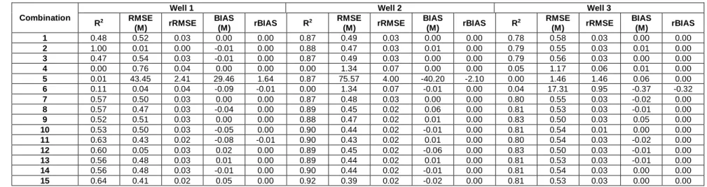
TABLE 3.3. EVALUATION CRITERIA OF CALIBRATION FOR GEP ...48
TABLE 3.4. EVALUATION CRITERIA OF VALIDATION FOR GEP ...49
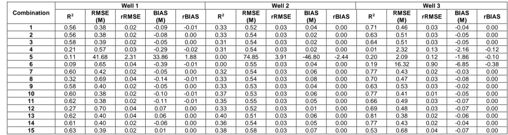
TABLE 3.5. EVALUATION CRITERIA OF CALIBRATION FOR M5 ...50
TABLE 3.6. EVALUATION CRITERIA OF VALIDATION FOR M5 ...51
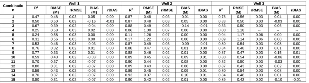
TABLE 3.7. EVALUATION CRITERIA OF CALIBRATION FOR WGEP ...52
TABLE 3.8. EVALUATION CRITERIA OF VALIDATION FOR WGEP ...53
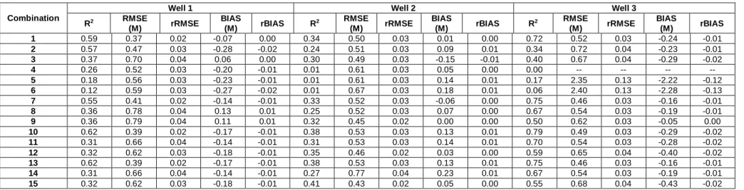
TABLE 3.9. EVALUATION CRITERIA OF CALIBRATION FOR WM5 ...54
TABLE 3.10. EVALUATION CRITERIA OF VALIDATION FOR WM5 ...55
TABLE 11 COMPARISON OF DIFFERENT MODELS ...56
TABLE 4.1. THE GEOGRAPHICAL COORDINATES OF THE STATIONS ...78
TABLE 4.2. EVALUATION CRITERIA OF THE SIMULATION FOR EEMD-GEP ...79
TABLE 4.3. EVALUATION CRITERIA OF THE SIMULATION FOR EEMD-M5 ...80
TABLE 4.4. COMPARISON OF DIFFERENT MODELS ...81
TABLE 2.1. RMSE, MAE, AND NS OF THE ORIGINAL ARTICLE AND THE PRESENT DISCUSSION SIMULATIONS ...92
LISTE DES FIGURES
FIG. 3.1: A) HAAR WAVELET. B) DB2 WAVELET. C) SYM3 WAVELET. D) COIF1 WAVELET.
E) DB4 WAVELET ...43
FIG. 3.2 SCHEMATIC DIAGRAM OF WGEP AND WM5 MODELS ...43
FIG. 3.3 LOCATION OF THE THREE OBSERVATION WELLS AND ONE METEOROLOGICAL STATION IN A) IRAN, B) LORESTAN PROVINCE, C) DELFAN PLAIN ...44
FIG. 3.4 TEMPERATURE TIME SERIES SUB-SIGNALS WITH THE WAVELET FUNCTION OF COIF1, LEVEL 8 ...44
FIG. 3.5 SIMULATED AND OBSERVED VALUES FOR A) WELL 1, B) WELL 2 AND C) WELL 3 ...46
FIG. 4.1 THE FLOWCHART OF THE EMD ALGORITHM ...76
FIG. 4.2 SIMULATED AND OBSERVED VALUES OF A) WELL 1, B) WELL 2 AND C) WELL 3 ...77
FIG. 2.1 SIMULATED AND OBSERVED RAINFALL FOR INNER TEST. ...93
FIG. 2.2 SIMULATED AND OBSERVED RAINFALL FOR THE OUTER TEST. ...93
LISTE DES ABRÉVIATIONS
Adaptive Neuro-Fuzzy Inference System ANFIA
Artificial Neural Network ANN
Biais moyen BIAS
Biais moyen relatif rBIAS
Classification et de régression CART
Coefficient de determination R2
Discrete Wavelet Transform DWT
Empirical Mode Decomposition EMD
Ensemble EMD EEMD
Gene Expression Programming GEP
Intelligence artificielle IA
Least Square Support Vector Machine ASSVM
M5 model tree M5
Mode intrinsèque IMF
Multivariate Adaptive Regression Splines MARS
Neuro-Fuzzy NF
Niveau d’eaux souterraines ES
Racine carrèe de l’erreur quadratique moyenne relative rRMSE
Racine carrée de l'erreur quadratique moyenne RMSE
Supportive Vector Machine SVM
1. INTRODUCTION
Les travaux de recherche présentés dans ce mémoire concernent la simulation du niveau d’eau souterraine (ES). Nos trois articles sont résumées dans cette partie.
Les eaux souterraines constituent l'une des principales sources d'approvisionnement en eau pour l'homme et constituent une variable importante pour les projets hydro-environnementaux (Nourani and Mousavi, 2016). L'étude des ES fournit aux chercheurs des informations pour gérer les ressources en eau (Barzegar et al., 2017). Il est donc nécessaire, il est nécessaire de simuler les ES pour étudier leur disponibilité pour les activités humaines.
Les modèles physiques et mathématiques ont été pris en compte dans de nombreuses études pour la simulation des ES. Ces modèles ont été largement utilisés, mais ils n'ont pas toujours fourni toutes les informations requises concernant la simulation des niveaux de ES (Nayak et al., 2006). Pour simuler les ES, les modèles physiques requièrent beaucoup de données de haute précision et ne conduisent pas toujours à de bonnes performances (Nayak et al., 2006; Shiri et al., 2013). Les modèles déterministes ont également besoin de beaucoup d'informations et peuvent mener à des équations difficiles à résoudre.
Pour adresser les limites des modèles physiques et mathématiques, un grand nombre de chercheurs ont utilisé des modèles d'intelligence artificielle (IA). Ces modèles ont relevé une capacité élevée de simulation des ES (Coppola et al., 2003; Lallahem et al., 2005;
Nayak et al., 2006; Sahoo et al., 2005). Parmi une gamme relativement large de modèles d'intelligence artificielle, le "Gene Expression Programming (GEP)" et le "M5 model tree (M5)" ont montré une grande capacité à simuler des phénomènes hydrologiques tels que des ES (Shiri and Kisi, 2011; Shiri et al., 2013).
Shiri and Kişi (2011) ont étudié l'aptitude du GEP et du "Adaptive Neuro-Fuzzy Inference System (ANFIS)" à la prévision des fluctuations des ES et ont constaté que le GEP
des ES et d'évaporation et ont conclu que le GEP conduit à de meilleures performances par rapport aux autres.
Solomatine and Xue (2004), pour la prévision des crues, etBhattacharya and Solomatine (2005), pour la relation niveau d'eau-débit, ont appliqué M5 et "Artificial Neural Network (ANN)" pour comparer la précision des modèles. Les études ont montré que M5 avait la même précision que les ANN, mais avec un certain nombre d'avantages, tels que la transparence, la vitesse de formation élevée et la convergence rapide.Kisi (2015) et Kisi (2016) ont utilisé "Least Square Support Vector Machine (LSSVM)", "Multivariate Adaptive Regression Splines (MARS)" et M5 pour analyser la précision des modèles de simulation d'évaporation et d'évapotranspiration, respectivement. L'auteur a défini différents scénarios pour analyser la précision des modèles et a conclu que chaque modèle peut avoir une bonne précision en modifiant les variables d'entrée.
Malgré la large application des modèles, ceux-ci risquent de ne pas être aussi efficaces pour modéliser des séries chronologiques comportant de fortes fluctuations non stationnaires (Nourani et al., 2009a). Ainsi, certaines méthodes ont été développées pour améliorer la capacité des modèles à simuler des séries temporelles hautement non stationnaires (Lee and Ouarda, 2012). Des méthodes telles que "Wavelet transform (WT)", "Empirical Mode Decomposition (EMD)" et "Ensemble EMD (EEMD)" ont été recommandées comme outil de prétraitement de la série chronologique afin d'améliorer la précision des modèles basés sur l'IA (Kisi and Shiri, 2011; Nourani et al., 2009b; Solgi et al., 2017; Wang et al., 2015).
WT a été développé pour pré-traiter un signal. Cette méthode a été adaptée par un grand nombre d'hydrologues pour décomposer une série chronologique en sous-séries (Oh et al., 2017; Ouachani et al., 2013; Shoaib et al., 2015; Sivapragasam et al., 2015). Shoaib et al. (2015) ont prévu le ruissellement en utilisant le modèle GEP combiné avec le WT. Les auteurs ont conclu que le WT améliore les performances du GEP.. Kisi and Shiri (2011) ont produit des modèles hybrides en combinant les modèles GEP et "Neuro-Fuzzy (NF)" pour la prévision des précipitations. Les résultats ont montré que WT améliore la précision des modèles et que GEP combiné à WT, est le modèle le plus précis.
EEMD est une méthode permettant de décomposer une série chronologique en composantes et convient au prétraitement de séries chronologiques non stationnaires (Wang et al., 2015). De nombreuses études prouvent que l'utilisation de EEMD augmente la précision de la modélisation (Lee and Ouarda, 2011; Lee and Ouarda, 2012; Masselot et al., 2018). Huang et al. (2014) ont produit un modèle hybride conçu par EEMD pour simuler le débit mensuel et ont indiqué que EEMD pouvait améliorer les résultats de la simulation. Dans une autre étude, Jiao et al. (2016) ont confirmé qu'un modèle hybride produit par EEMD avait la capacité de simuler des données hydrologiques.
1.1. PROBLÈME
Comme les ES constituent une variable non linéaire et que les chercheurs n'ont pas accès à toutes les variables affectives sur les ES dans les conditions réelles, les modèles physiques et mathématiques peuvent ne pas aboutir à une simulation avec une bonne précision.
1.2. HYPOTHÈSE
Les modèles basés sur l'IA peuvent être utiles pour la simulation des ES et leurs combinaisons avec WT et EEMD pourrait améliorer leur précision.
1.3. OBJECTIFS
L'objectif principal de cette étude est de présenter un modèle permettant de simuler les ES avec une grande précision. Le modèle devrait dépasser les limites imposées à la simulation de séries chronologiques hautement non stationnaires.
1.4. ORIGINALITÉ
À la connaissance de l'auteur, il n'y a pas eu d'étude combinant GEP et M5 avec EEMD pour la simulation ES.
1.5. ORGANISATION DE LA SYNTHÈSE
La présente synthèse est divisée en cinq parties principales. La section 1 présente l'introduction. La section 2 explique les méthodes. La section 3 donne les informations sur l’étude de cas et les données utilisées. La section 4 indique les résultats. La section 5 présente les conclusions et recommandations.
2. MÉTHODES
Dans la présente étude, deux modèles appelés GEP et M5 et deux méthodes appelées WT et EEMD sont appliqués à la simulation des ESs.. Pour ce faire, on prend en compte les séries temporelles de précipitations mensuelles et de température de l'air d'une station météorologique, ainsi que les séries temporelles des niveaux d’ES de trois puits d'observation situés dans la plaine de Delfan, située au nord de la province de Lorestan, en Iran. Ensuite, chaque série temporelle est décomposée en sous-signaux par WT et EEMD. Les sous-signaux générés par WT sont utilisés pour produire des modèles hybrides appelés WGEP et WM5. Les sous-signaux produits par EEMD sont appliqués pour former des modèles hybrides appelés EEMD-GEP et EEMD-M5. Enfin, les valeurs de simulation utilisant des modèles hybrides et simples sont évaluées selon différents critères pour déterminer le modèle à grande précision.
Les algorithmes et les formules de modèles et de méthodes sont présentés dans les articles. Dans les parties suivantes, un résumé des modèles et méthodes utilisés est présenté.
2.1. GENE EXPRESSION PROGRAMING (GEP)
GEP a été introduit par Ferreira (2001) et fait partie des algorithmes évolutifs. Les algorithmes évolutifs imitent le mécanisme des organismes vivants. L'avantage de GEP par rapport à d'autres modèles tels que ANN est que la structure optimale du modèle est déterminée pendant le processus de formation.
solution est présentée. Dans le cas de non satisfaction de la solution attendue, l'évolution de la population continue à améliorer les solutions.
2.2. M5 MODEL TREE (M5)
Quinlan (1992) a présenté le M5 en développant un "Decision Tree". M5 établit une relation entre les variables dépendantes et indépendantes en présentant des règles incluant des régressions linéaires. L'avantage de M5 par rapport aux arbres de classification et de régression (CART) est que M5 produit un arbre plus petit et est plus précis (Quinlan, 1992).
M5 utilise une approche descendante pour aller d'un nœud en haut à une feuille en bas et son algorithme comporte deux étapes. Quinlan (1992) explique qu'à la première étape, un critère de scission est appliqué pour construire un arbre. Le critère de division explique le taux d'erreur au nœud et repose sur la minimisation de l'écart type des nœuds. À la deuxième étape, l’algorithme de Quinlan (1992) est utilisé pour élaguer les branches et les remplacer par des modèles de régression linéaire.
2.3. WAVELET TRANSFORM (WT)
WT a été présenté par Grossmann and Morlet (1984) dans la discipline des géosciences. Le WT est une méthode de traitement permettant d'extraire des informations cachées d'une série chronologique. Pour des applications pratiques, les hydrologues ont accès à des signaux de temps discrets (Nourani et al., 2014). Ainsi, Mallat (1989) a introduit une extension discrète de WT appelée "discrete wavelet transform (DWT)".
Mallat (1989) a mis au point la technologie DWT en utilisant des filtres passe haut et passe bas. Dans le DWT, pour le premier niveau de décomposition, un signal est décomposé en une approximation (A) et en détail (d) par les filtres. L'approximation traitée est ensuite appliquée de façon itérative aux décompositions résultantes (Mallat, 1989).
2.4. EMPIRICAL MODE DECOMPOSITION (EMD)
Huang et al. (1998) ont introduit l'EMD en tant que méthode pour décomposer une série chronologique en composantes de fréquence. Les principales différences entre EMD et WT sont qu’EMD extrait les caractéristiques d’une série chronologique sans présupposition et est capable de reconnaître la fréquence instantanée de la série chronologique.
Les composantes de fréquence appelées fonctions de mode intrinsèque (IMF) ont deux caractéristiques (Lee and Ouarda, 2012). Premièrement, le nombre d’extrema locaux doit
être égal au nombre de passages par zéro ou en diffèrer au plus par un. Deuxièmement, la moyenne des enveloppes supérieure et inférieure, calculée par les maxima et les minima locaux, devrait être égale à zéro.
Le processus de calcul des IMF est le suivant : d’abord, déterminer les minima et les maxima locaux. Deuxièmement, adapter les enveloppes supérieure et inférieure aux maxima et minima locaux, respectivement, par splines cubiques. Troisièmement, soustraire la moyenne des enveloppes supérieure et inférieure de la série temporelle à tout emplacement temporel pour calculer la première composante. Quatrièmement, calculer Dk comme critère d'arrêt. Avec Dk=∑ |ℎ1
𝑘−1(𝑡)−ℎ
1𝑘(𝑡)|2 𝑇
𝑡=0
∑𝑇𝑡=0|ℎ1𝑘−1(𝑡)|2 où k est le numéro de
répétition additionnelle pour le processus de tamisage. Si Dk est supérieur à 0,2, la série temporelle est remplacée par le signal calculé à partir de la troisième étape. Ensuite, le processus est répété à partir de la première étape. Si Dk est inférieur à 0,2, le signal calculé est appelé le premier FMI. Cinquièmement, définir le résidu en soustrayant le signal calculé de la série temporelle. Si le résidu satisfait aux caractéristiques des IMF, il est considéré comme une série chronologique et les étapes 1 à 4 sont extraites pour produire le prochain FMI. En cas de non-satisfaction de la condition, l'algorithme est arrêté.
L'algorithme EMD peut causer des problèmes de mélange de modes (Lee and Ouarda, 2010; Wang et al., 2015). Pour résoudre le problème, Wu and Huang (2009) ont développé EMD en ajoutant des bruits blancs finis à la série chronologique ciblée et l'ont
appelé ensemble EMD (EEMD). Dans le système EEMD, le nombre d'ensembles ajoutés (𝜀) et l'amplitude du bruit devraient être prescrits.
2.5. CRITÈRE D'ÉVALUATION
Dans la présente étude, le coefficient de détermination (R2), la racine carrée de l'erreur quadratique moyenne (RMSE), la racine carrée de l’erreur quadratique moyenne relative (rRMSE), le biais moyen (BIAS) et le biais moyen relatif (rBIAS) sont utilisés pour évaluer les performances des modèles.
3. ZONE D'ÉTUDE
Les méthodes sont appliquées aux données de la plaine de Delfan, située au nord de la province du Lorestan, en Iran. La plaine est située entre 47°, 21' et 48°, 21' E à 33°, 48' et 34°, 22' N, entre 1700 et 2100 mètres d'altitude. Les valeurs mensuelles de ES (m), de précipitation (mm) et température de l'air (°C) sont utilisées pour simuler ES un mois à l'avance. Dans la présente étude, des décalages sont appliqués aux variables d’entrée. Le décalage dans le temps signifie l'utilisation des valeurs des variables correspondant aux mois précédents. Le décalage temporel 1 fait référence aux variables correspondant au mois précédent, le décalage temporel 2 aux variables correspondant à il y a deux mois.
La série d'observations est divisée en deux parties. La première partie, comprenant 75% de la série, est utilisée pour l'étalonnage et la seconde partie, comprenant 25%, est utilisée pour la validation.
4. RÉSULTATS
Les résultats de cette étude sont résumés dans le paragraphe suivant. En premier lieu nous présentons les résultats des modèles simples, GEP et M5. Ensuite nous résumons ceux des modèles hybrides.
puits 2. Les résultats indiquent que, pour différentes combinaisons de variables, les précipitations ne sont pas une variable efficace pour la simulation, tandis que la température de l’air et les ES jouent un rôle important dans la simulation.
Pour tous les puits d'observation, les modèles hybrides produits par WT donnent de meilleures performances que GEP et M5. Les performances de WGEP et WM5 sont proches. Pour le puits 1, les résultats de calibration sont proches, mais pour la validation, WM5 performe légèrement mieux que WGEP. Pour le puits 2, les résultats de validation de WGEP montrent une meilleure performance que WM5. Pour le puits 3, WGEP est un peu meilleur que WM5 pour l’étalonnage et la validation.
Pour le puits 1, les performances du modèle EEMD-GEP produisent la meilleure précision en utilisant ε = 0,3. Pour les puits 2 et 3, ε = 0,2 indique la plus grande précision. Les critères d'évaluation de EEMD-M5 indiquent que ses performances sont trop faibles et que le modèle n'est pas adapté à la simulation.
On peut comprendre de la comparaison des modèles que les modèles hybrides générés par WT ont de meilleures performances que les modèles hybrides générés par la méthode EEMD. Pour le puits 1, WM5 peut être sélectionné comme le meilleur modèle pour la simulation. En ce qui concerne le puits 2, le WGEP indique les résultats les plus appropriés. Pour le puits 3, WGEP et WM5 ont des performances proches et sont meilleures que EEMD-GEP et EEMD-M5.
5. CONCLUSIONS ET RECOMMENDATIONS
Dans la présente étude, les modèles GEP et M5 sont utilisés pour la simulation. Des modèles WT, ainsi que EEMD, sont appliqués pour produire des modèles hybrides. Cette étude inclut également une discussion sur l'article de Du et al. (2017) sur l'utilisation correcte de l'application de WT. La conclusion de la discussion est également résumée à la fin de cette section. Cette partie présente le résumé des articles.
En se basant sur les résultats des modèles, on peut conclure que, pour prétraiter et simuler les séries temporelles de ES, le WT et le GEP, respectivement, produisent des
Les résultats de modèles simples démontrent que la sélection d'un temps de latence approprié pour les valeurs d'entrée joue un rôle important dans la simulation. Si un grand nombre de temps de latence est utilisé, le temps de simulation augmente, alors que les temps de latence ne sont pas toujours utiles pour améliorer la précision.
Les résultats des modèles hybrides à différents niveaux de la décomposition indiquent que la sélection d'un niveau de décomposition approprié affecte la précision des modèles hybrides.. Un niveau élevé de décomposition n'est pas toujours utile pour augmenter la précision du modèle. Un niveau de décomposition optimal doit être sélectionné.
Les résultats des modèles hybrides intégrés à EEMD présentent l'importance de ε dans la méthode EEMD et son impact sur la précision des modèles hybrides.
En outre, on peut conclure que les valeurs de température de l'air et des ES sont des variables plus efficaces que les valeurs de précipitation pour la simulation des ES dans cette région de l'Iran. Cela signifie que la sélection de variables hydrologiques en tant qu'entrées dans les modèles est très spécifique à la région d'étude et au climat en question, et affecte de manière significative les performances des modèles.
Dans le présent travail, la simulation des ES a été envisagée à l'aide de modèles simples et hybrides. Il serait intéressant d’évaluer la capacité de ces modèles à prédire à long terme les ES. Ceci est important car la gestion efficace d'un certain nombre de problèmes environnementaux (tels que les sécheresses) nécessite un plan à long terme.
Pour améliorer les méthodes d’EEMD, de nouvelles techniques telles que "Complementary Ensemble Mode Decomposition" et "Partly Ensemble Mode Decomposition" ont été développées. Il est suggéré d'étudier la capacité des nouvelles techniques à produire des modèles hybrides pour la simulation des ES.
Dans la discussion, les mêmes données de Du et al (2017) sont utilisées pour vérifier la validité des affirmations des auteurs. La seule différence entre l'analyse effectuée dans la présente discussion et dans l'article initial est l'utilisation des décalages temporels appliqués aux entrées des modèles. Les résultats montrent que si les décalages
série chronologique par WT ne donne pas de faux résultats. Par conséquent, l'affirmation de Du et al. (2017) n'a pas pu être vérifiée pour DWT-ANN.
6. RÉFÉRENCES
[1] Barzegar R, Fijani E, Asghari Moghaddam A, Tziritis E (2017) Forecasting of groundwater level fluctuations using ensemble hybrid multi-wavelet neural network-based models. Science of The Total Environment. 599-600:20-31. doi:https://doi.org/10.1016/j.scitotenv.2017.04.189
[2] Bhattacharya B, Solomatine DP (2005) Neural networks and M5 model trees in modelling water level–discharge relationship. Neurocomputing. 63:381-396. doi:https://doi.org/10.1016/j.neucom.2004.04.016
[3] Coppola E, Szidarovszky F, Poulton M, Charles E (2003) Artificial Neural Network Approach for Predicting Transient Water Levels in a Multilayered Groundwater System under Variable State, Pumping, and Climate Conditions. Journal of Hydrologic Engineering. 8:348-360. doi:10.1061/(ASCE)1084-0699(2003)8:6(348)
[4] Ferreira C (2001) Gene Expression Programming: A New Adaptive Algorithm for Solving Problems vol 13. Complex Systems Publications, Angra do Heroísmo, Portugal.
[5] Ferreira C (2006) Gene Expression Programming Mathematical Modeling by an Artificial Intelligence. Studies in Computational Intelligence, vol 21. Springer-Verlag Berlin Heidelberg, Germany. doi:10.1007/3-540-32849-1
[6] Grossmann A, Morlet J (1984) Decomposition of Hardy Functions into Square Integrable Wavelets of Constant Shape SIAM. Journal on Mathematical Analysis 15:723-736. doi:10.1137/0515056
[7] Huang NE et al. (1998) The empirical mode decomposition and the Hilbert spectrum for nonlinear and non-stationary time series analysis Proceedings of the Royal Society of London Series A: Mathematical, Physical and Engineering Sciences. 454:903-995. doi:10.1098/rspa.1998.0193
[8] Huang S, Chang J, Huang Q, Chen Y (2014) Monthly streamflow prediction using modified EMD-based support vector machine. Journal of Hydrology. 511:764-775 doi:https://doi.org/10.1016/j.jhydrol.2014.01.062
[9] Jiao G, Guo T, Ding Y (2016) A New Hybrid Forecasting Approach Applied to Hydrological Data: A Case Study on Precipitation in Northwestern China Water. 8:367
[10] Kisi O (2015) Pan evaporation modeling using least square support vector machine, multivariate adaptive regression splines and M5 model tree. Journal of Hydrology. 528:312-320. doi:https://doi.org/10.1016/j.jhydrol.2015.06.052
[11] Kisi O (2016) Modeling reference evapotranspiration using three different heuristic regression approaches Agricultural. Water Management. 169:162-172 doi:https://doi.org/10.1016/j.agwat.2016.02.026
[12] Kisi O, Shiri J (2011) Precipitation Forecasting Using Wavelet-Genetic Programming and Wavelet-Neuro-Fuzzy Conjunction Models. Water Resources Management. 25:3135-3152. doi:10.1007/s11269-011-9849-3
[13] Lallahem S, Mania J, Hani A, Najjar Y (2005) On the use of neural networks to evaluate groundwater levels in fractured media. Journal of Hydrology. 307:92-111. doi:http://dx.doi.org/10.1016/j.jhydrol.2004.10.005
[14] Lee T, Ouarda TBMJ (2010) Long-term prediction of precipitation and hydrologic extremes with nonstationary oscillation processes. Journal of Geophysical Research: Atmospheres. 115: D13107. doi:10.1029/2009JD012801
[15] Lee T, Ouarda TBMJ (2011) Prediction of climate nonstationary oscillation processes with empirical mode decomposition. Journal of Geophysical Research: Atmospheres. 116: D06107. doi:10.1029/2010JD015142
[16] Lee T, Ouarda TBMJ (2012) Stochastic simulation of nonstationary oscillation hydroclimatic processes using empirical mode decomposition. Water Resources Research. 48: W02514. doi:10.1029/2011WR010660
[17] Mallat SG (1989) A theory for multiresolution signal decomposition: the wavelet representation. IEEE Transactions on Pattern Analysis and Machine Intelligence. 11:674-693. doi:10.1109/34.192463
[18] Masselot P, Chebana F, Bélanger D, St-Hilaire A, Abdous B, Gosselin P, Ouarda TBMJ (2018) EMD-regression for modelling multi-scale relationships, and application to weather-related cardiovascular mortality. Science of The Total Environment. 612:1018-1029. doi:https://doi.org/10.1016/j.scitotenv.2017.08.276
[19] Nayak PC, Rao YRS, Sudheer KP (2006) Groundwater Level Forecasting in a Shallow Aquifer Using Artificial Neural Network Approach. Water Resources Management. 20:77-90. doi:10.1007/s11269-006-4007-z
[20] Nourani V, Alami MT, Aminfar MH (2009a) A combined neural-wavelet model for prediction of Ligvanchai watershed precipitation. Engineering Applications of
Artificial Intelligence. 22:466-472.
doi:https://doi.org/10.1016/j.engappai.2008.09.003
[21] Nourani V, Hosseini Baghanam A, Adamowski J, Kisi O (2014) Applications of hybrid wavelet–Artificial Intelligence models in hydrology: A review. Journal of Hydrology. 514:358-377. doi:https://doi.org/10.1016/j.jhydrol.2014.03.057
[22] Nourani V, Komasi M, Mano A (2009b) A Multivariate ANN-Wavelet Approach for Rainfall–Runoff Modeling. Water Resources Management. 23:2877. doi:10.1007/s11269-009-9414-5
[23] Nourani V, Mousavi S (2016) Spatiotemporal groundwater level modeling using hybrid artificial intelligence-meshless method. Journal of Hydrology. 536:10-25. doi:https://doi.org/10.1016/j.jhydrol.2016.02.030
[24] Oh Y-Y, Yun S-T, Yu S, Hamm S-Y (2017) The combined use of dynamic factor analysis and wavelet analysis to evaluate latent factors controlling complex groundwater level fluctuations in a riverside alluvial aquifer. Journal of Hydrology. 555:938-955. doi:https://doi.org/10.1016/j.jhydrol.2017.10.070
[25] Ouachani R, Zoubeida B, Taha O (2013) Power of teleconnection patterns on precipitation and streamflow variability of upper Medjerda Basin International. Journal of Climatology. 33:58-76. doi:doi:10.1002/joc.3407
[26] Quinlan JR (1992) Learning with Continuous Classes Proceedings of Australian. Joint Conference on Artificial Intelligence, Hobart, Australia, World Scientific, Singapore:343-348
[27] Sahoo GB, Ray C, Wade HF (2005) Pesticide prediction in ground water in North Carolina domestic wells using artificial neural networks. Ecological Modelling 183:29-46. doi:http://dx.doi.org/10.1016/j.ecolmodel.2004.07.021
[28] Shiri J, Kişi Ö (2011) Comparison of genetic programming with neuro-fuzzy systems for predicting short-term water table depth fluctuations. Computers & Geosciences. 37:1692-1701 doi:http://dx.doi.org/10.1016/j.cageo.2010.11.010
[29] Shiri J, Kisi O, Yoon H, Lee K-K, Hossein Nazemi A (2013) Predicting groundwater level fluctuations with meteorological effect implications—A comparative study among soft computing techniques. Computers & Geosciences. 56:32-44. doi:https://doi.org/10.1016/j.cageo.2013.01.007
[30] Shoaib M, Shamseldin AY, Melville BW, Khan MM (2015) Runoff forecasting using hybrid Wavelet Gene Expression Programming (WGEP) approach. Journal of Hydrology. 527:326-344. doi:http://dx.doi.org/10.1016/j.jhydrol.2015.04.072
[31] Sivapragasam C, Kannabiran K, Karthik G, Raja S (2015) Assessing Suitability of GP Modeling for Groundwater Level. Aquatic Procedia. 4:693-699 doi:https://doi.org/10.1016/j.aqpro.2015.02.089
[32] Solgi A, Pourhaghi A, Bahmani R, Zarei H (2017) Pre-processing data using wavelet transform and PCA based on support vector regression and gene expression programming for river flow simulation. Journal of Earth System Science. 126:65. doi:10.1007/s12040-017-0850-y
[33] Solomatine DP, Xue Y (2004) M5 Model Trees and Neural Networks: Application to Flood Forecasting in the Upper Reach of the Huai River in China. Journal of
Hydrologic Engineering. 9:491-501. doi:doi:10.1061/(ASCE)1084-0699(2004)9:6(491)
[34] Wang W-c, Chau K-w, Xu D-m, Chen X-Y (2015) Improving Forecasting Accuracy of Annual Runoff Time Series Using ARIMA Based on EEMD Decomposition. Water Resources Management. 29:2655-2675. doi:10.1007/s11269-015-0962-6 [35] Wu Z, Huang NE (2009) ENSEMBLE EMPIRICAL MODE DECOMPOSITION: A
NOISE-ASSISTED DATA ANALYSIS METHOD. Advances in Adaptive Data Analysis. 01:1-41. doi:10.1142/s1793536909000047
PARTIE II: ARTICLES
CHAPITRE II: GROUNDWATER LEVEL SIMULATION USING
GENE EXPRESSION PROGRAMMING AND M5 MODEL TREE
Groundwater level simulation using Gene Expression Programming
and M5 Model tree combined with wavelet transform
Ramin Bahmani1, Abazar Solgi2, Taha B. M. J. Ouarda1
1 Canada Research Chair in Statistical Hydro-climatology, INRS-ETE, Québec (Québec), Canada.
2 Department of Water Resources Engineering, Faculty of Water Sciences Engineering, Shahid Chamran University of Ahvaz, Ahvaz, Iran
Abstract
In order to understand and adequately manage hydrological stress, it is necessary to simulate the groundwater level accurately. In the present research, Gene Expression Programming (GEP) and M5 model tree (M5) are used to simulate monthly groundwater levels. The models are combined with wavelet transform to produce two hybrid models: Wavelet Gene Expression Programming (WGEP) and Wavelet M5 model tree (WM5). For the simulation, groundwater level, temperature and precipitation values from three observation wells and one meteorological station, located in the Delfan plain (Nourabad), Iran, are used. The results indicate that the hybrid models, WGEP and WM5, have better performance than simple models, GEP and M5. The performances of the two hybrid models are similar. It is also observed that selecting a suitable time lag for inputs plays an important role in the accuracy of the simple models. The selection of a suitable decomposition level strongly affects the accuracy of hybrid models.
Keywords: Groundwater level; Gene Expression Programming; Hybrid model; M5 Model tree; Wavelet transform.
Abbreviations
GEP Gene Expression Programming
M5 M5 model tree
WGEP Wavelet Gene Expression Programming
WM5 Wavelet M5 model tree
ANFIS Adaptive Neuro-Fuzzy Inference System ANN Artificial Neural Network
LSSVM Least Square Support Vector Machine MARS Multivariate Adaptive Regression Splines
WT Wavelet Transform
NF Neuro-Fuzzy
RMSE Root Mean Squared Error
rRMSE Relative Root Mean Squared Error
BIAS Mean Bias
1. Introduction
Measuring groundwater levels, using observation wells, is one of the main resources for investigating hydrological stresses and is necessary to understand groundwater fluctuations in arid and semi-arid areas (Barzegar et al., 2017; Ebrahimi and Rajaee, 2017). The investigation of groundwater levels provides key information to managers for decision making during extreme conditions such as droughts (Barzegar et al., 2017;
Reghunath et al., 2005).
To simulate groundwater levels, physical models have been considered by a number of researchers. Although these models have been widely used, they have not always provided all required information concerning groundwater level simulation (Bierkens, 1998; Nayak et al., 2006). Compared to statistical approaches, physical models require much more high accuracy data for simulating groundwater levels and do not always lead to good performances in establishing non-linear relationships between variables (Nayak et al., 2006; Shiri et al., 2013).
To solve the problem, Artificial Intelligence (AI) models have been considered for simulating groundwater levels and several studies have reported the good ability of AI-based models to simulate groundwater levels (Coppola et al., 2003; Lallahem et al., 2005;
Nayak et al., 2006; Sahoo et al., 2005). Among a relatively wide range of AI models, Gene Expression Programming (GEP) has particularly shown a high ability to efficiently simulate groundwater levels. For instance, Shiri and Kişi (2011) investigated the ability of GEP and the Adaptive Neuro-Fuzzy Inference System (ANFIS) for forecasting water table fluctuations and found that the models have a good ability to forecast the fluctuations, with the GEP leading to better results than the ANFIS. Again, Shiri et al. (2013) simulated groundwater level fluctuations by considering the meteorological effects using GEP, Supportive Vector Machine, and ANFIS models. The authors used different combinations of precipitation, groundwater level, and evaporation values for simulation and concluded that GEP leads to better performances than the other methods.
being black box models with which it is hard to understand the dynamics and the effects of different variables on the simulation output (Liao and Sun, 2010; Solomatine and Xue, 2004). Hence, transparent models such as M5 model tree (M5), which produces explicit equations, have been proposed for simulation purposes (Keshtegar et al., 2016; Raza, 2015).
The M5 model has been successfully used for simulating hydrological variables. For instance, Liao and Sun (2010) used the improved decision tree model to predict water quality. The authors found the decision tree method to be more accurate and easier to use than Artificial Neural Networks (ANNs). They concluded that improved decision tree models, which integrate some of the ANN characteristics in the main decision tree methods, were suitable for their research field. Solomatine and Xue (2004) used M5 and ANN to compare the accuracy of models for flood forecasting. The study reported that M5 has the same accuracy than ANNs but with a number of advantages, such as transparency, high speed of training, and fast convergence. In another study,
Bhattacharya and Solomatine (2005) used ANN and an M5 to develop models of the water level-discharge relationship. They concluded that both ANN and M5 models were better than the traditional rating curve, using the same data. In more recent research, Kisi (2015) used Least Square Support Vector Machine (LSSVM), Multivariate Adaptive Regression Splines (MARS) and M5 to analyze the accuracy of the models for simulating pan evaporation. The author defined different scenarios to analyze the accuracy of the models and concluded that, when the local input and output data are used, LSSVM has the best results, whereas MARS leads to a better performance when the local input and output data are not considered. Kisi (2016) used the same models to simulate evapotranspiration and concluded that LSSVR, MARS, and M5 are suitable for simulation with the local input and output, without local input, and without the local input and output values respectively. Kisi and Parmar (2016) used the same models to simulate river water pollution and concluded that MARS and LSSVM are suitable to model river water pollution.
The literature indicates that GEP and M5 have a high ability to adequately simulate hydrologic time series. However, when hydrologic phenomena are highly non-stationary
et al., 2014). In this case, wavelet transform (WT) can be recommended as a tool for pre-processing the time series in order to increase the accuracy of AI-based models (Nourani et al., 2009a; Solgi et al., 2017c). WT helps hydrologists decompose a time signal into sub-signals allowing the models to capture information with different resolution levels (Nourani et al., 2009b).
WT was presented by Grossmann and Morlet (1984) in the field of geoscience and has been adapted for the pre-processing of time series in hydrology (Oh et al., 2017;
Ouachani et al., 2013; Shoaib et al., 2015; Sivapragasam et al., 2015; Solgi et al., 2017a).
Partal and Kişi (2007) used WT to decompose daily precipitation time series to sub-signals. Then, the sub-signals were entered as inputs to a Neuro-Fuzzy (NF) model to forecast precipitation. The authors reported that, when WT was used, the NF model led to a better fit with observed values. Shoaib et al. (2015) combined GEP with WT to predict runoff and concluded that using WT improves the performance of GEP. Kisi and Shiri (2011) used GEP and NF models to forecast precipitation, and also combined the models with WT to produce hybrid models. The authors concluded that hybrid models were more accurate than simple models and GEP combined with WT led to best results.
Very few studies have used GEP and M5 in combination with WT to simulate groundwater levels. The first objective of the present study is to simulate monthly groundwater levels using GEP and M5. The models are also combined with WT (the resulting models are called WGEP and WM5) to produce hybrid models for groundwater level simulation. For the simulation using simple models, different combinations of groundwater level, precipitation and temperature time series are used. For the simulation using hybrid models, the time series is decomposed to sub-signals using WT. Then, the sub-signals are used as inputs to the GEP and M5 models. Finally, the performances of simple and hybrid models are compared to evaluate their performance.
The present paper is structured as follows. Section 2 provides a review of the theoretical background of the models used in this study, as well as the methodology adopted to produce the hybrid models and to compare the performances of the various models.
2. Methods
2.1. Gene Expression Programing (GEP)
GEP was first introduced by Ferreira (2001) and is part of what is called “evolutionary
algorithms”. Evolutionary algorithms, inspired by the Darwinian evolution theory, are algorithms that imitate the mechanism of living organisms. GEP differs from other models such as ANN, in that the structure, including the input variables, target and position function, are firstly defined. Then, the optimal structure of the model and coefficients are determined during the training process, whereas in the ANN model, the structure must be determined and only the coefficients of the model are obtained during the training process. This helps provide more flexibility to the GEP model and generally represents an advantage. The general process of solving a problem with GEP is briefly illustrated by the following steps.
1. Select a terminal set, which includes dependent and independent values. In this step, the root mean square error, as the fitness function, is used.
2. Choose a set of functions which includes arithmetic operators, test functions, and Boolean functions. The 10 used mathematical operators are multiplication, division, addition, subtraction, exponential, square root, natural logarithm, x to the power of 2, cube root, and inverse. The arithmetic operators of addition, subtraction, and multiplication are the most common types.
3. Obtain the accuracy index of the model which indicates the model ability to solve a specific problem.
4. Select stopping criteria, which are measures for stopping the program and obtaining the results, such as generated numbers or the maximum fixation.
5. Determine the control components, including numerical values and qualitative variables. These are used for controlling the program.
The present paper does not delve into the detailed theory of GEP. For more information, the reader is referred to Ferreira (2001), Ferreira (2002), and Ferreira (2006).
2.2. M5 Model Tree (M5)
The M5 Model Tree (M5) was introduced by Quinlan (1992) based on the Decision Tree method. The main advantage of M5 is that it presents a set of linear regressions that show the relationships between dependent and independent variables and they are interpretable (Raza, 2015). The M5 model lies between linear models, like ARIMA, and non-linear models, like ANNs (Solomatine and Xue, 2004). M5 includes a root, branches, nodes, and leaves like a tree and is drawn using top-down approach. The root as the first node is on the top and the tree grows down by nodes and branches to reach leaves. In M5, every leaf is a linear regression. Building the M5 model involves two steps. The first step consists in building a tree using a splitting criterion. The second step consists in pruning branches and replacing them with linear regression models.
2.2.1 Splitting criterion
The splitting criterion explains the rate of errors at the node and is based on minimizing the standard deviation of nodes. Because of the splitting process, the standard deviation in a given node, called child node, is generally smaller than the standard deviation in the previous node, called parent node (Kisi, 2015). A node ends in a leaf when minimizing standard deviation in the node is not possible. For the calculation of the reduction in standard deviation, the following equation is used (Quinlan, 1992):
𝑆𝐷𝑅 = 𝑠𝑑(𝑇) − ∑|𝑇𝑖|
|𝑇|𝑠𝑑(𝑇𝑖) (1)
where SDR is the reduction of standard deviation in a given node, T is a set of training data that reaches the parent node; Ti is a subset of the training data having the ith outcome
of the potential set, and sd is the standard deviation (Kisi, 2015). The M5 model selects the minimum expected error for each attribute at that node. For more details concerning the splitting criterion, the reader is referred to Quinlan (1986) and Quinlan (1992).
Secondly, it prunes the branches which do not increase the accuracy of the model. Finally, after the pruning, smoothing is needed to smooth sharp dissociation (Bhattacharya and Solomatine, 2005; Solomatine and Xue, 2004). For more details concerning the general M5 model, the reader is referred to (Quinlan, 1992).
2.3 Wavelet transform (WT)
The application of the wavelet transform (WT) in the geoscience discipline was introduced by Grossmann and Morlet (1984). The WT is an effective digital signal processing technique to extract hidden information form a signal. The WT was formulated as the continuous wavelet transform (CWT) by Mallat (1989) as follow:
𝐶𝑊𝑇 = ∫ 𝑓(𝑡). 𝜓∗(𝑡). 𝑑(𝑡)
+∞
−∞
(2)
where f(t) is the continuous signal, 𝜓(𝑡) is the wavelet function or mother wavelet and * refers to the complex conjugate. A mother wavelet has three characteristics: 1) limited number of fluctuations, 2) quick return to zero in both positive and negative directions in its domain and 3) zero average (Thuillard, 2001).
A mother wavelet is defined as (Oh et al., 2017):
𝜓(𝑎,𝑏)(𝑡) = |𝑎|−0.5𝜓 (
𝑡 − 𝑏
𝑎 ) , 𝑎 ∈ 𝑅, 𝑏 ∈ 𝑅, 𝑎 ≠ 0 (3)
where a is a dilation factor, b is a temporal translation, and R is the domain of real numbers.
For practical applications, hydrologists and modelers in general often have access to discrete time signals (Nourani et al., 2014). Therefore, a discrete extension of equation (2) called “discrete wavelet transform” (DWT) was proposed. The DWT is defined by (Kisi and Shiri, 2011):
𝐷𝑊𝑇 (𝑎, 𝑏) = 2−𝑗2∫ 𝜓∗( 𝑗=𝐽
where f(t) is a discrete time series at any time t, . j and k are integers which respectively control the wavelet dilation and the translation.
By using high-pass and low-pass filters, Mallat (1989) developed a way to implement the DWT. In the DWT, for the first decomposition level, a signal is decomposed to an approximation (A) and detail (d). The processed approximation is then applied to consequent decompositions iteratively (Mallat, 1989).
2.3.1 Choice of a mother wavelet
The main consideration for selecting a mother wavelet is the type of the time series. The main features of a mother wavelet include the region of support, associated with the wavelet span length, and the number of vanishing moments, limiting the ability of a wavelet to show information in a time series. In the present work, the Haar, Coif1, Sym3, Db4, and Db2 wavelets, which are well-known and commonly used in hydrological studies, are adopted for decomposing time signals(Nourani et al., 2014; Shoaib et al., 2015; Solgi et al., 2017b). Fig. 1 illustrates the graph of the mother wavelets.
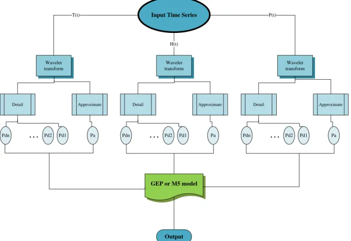
2.4 Hybrid Wavelet M5 model tree (WM5) and Wavelet Gene Expression Programming Models (WGEP) development
To develop hybrid models with the wavelet transform, the following steps are carried out. The groundwater level, temperature and precipitation time series are decomposed to sub-signals using DWT for different decomposition levels. Then, the sub-sub-signals are used as inputs into the GEP and M5 models, hence called WGEP and WM5. Fig. 2 presents the schematic diagram for producing WGEP and WM5 models. In this figure, P(t), T(t), and H(t) refer to the precipitation, temperature, and groundwater level time series respectively. The sub-signals of Pa, Ta, and Ha refer to the approximation of the final decomposition level. The sub-signals of Pd1 to Pdn, Td1 to Tdn and Hd1 to Hdn refer to the details of the decomposition from level 1 to the last decomposition level.
To determine the level of decomposition (L), the suggested equation of Nourani et al. (2009b) is used.
where L is the proposed decomposition level and N is the number of observed values.
2.5 Evaluation Criteria
Evaluation criteria serve to estimate the errors of the models according to the observed and simulated values. In the present paper, the following criteria are used to evaluate the models (Chebana et al., 2014):
a- The coefficient of determination or R2:
𝑅2 = 1 −∑(𝐻𝑜𝑏𝑠 − 𝐻𝑒𝑠𝑡) 2
∑(𝐻𝑜𝑏𝑠 − 𝐻̅)2 (6)
b- The root mean square error (RMSE):
𝑅𝑀𝑆𝐸 = √∑(𝐻𝑜𝑏𝑠− 𝐻𝑒𝑠𝑡)
2
𝑛 (7)
c- The relative root mean square error (rRMSE):
𝑟𝑅𝑀𝑆𝐸 = 100√
∑(𝐻𝑜𝑏𝑠 − 𝐻𝑒𝑠𝑡
𝐻𝑜𝑏𝑠 )2 𝑛
(8)
d- The mean bias (BIAS):
𝐵𝐼𝐴𝑆 = ∑(𝐻𝑜𝑏𝑠 − 𝐻𝑒𝑠𝑡)
𝑛 (9)
e- The relative mean bias (rBIAS)
𝑟𝐵𝐼𝐴𝑆 = 100 ∗ (
∑ (𝐻𝑜𝑏𝑠− 𝐻𝑒𝑠𝑡
𝐻𝑜𝑏𝑠 )
𝑛 )
(10)
where Hobs refers to the observed values, Hest refers to the estimated values, H̅ is the average of observed values and n is the number of observations.
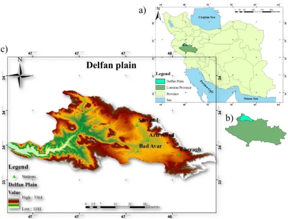
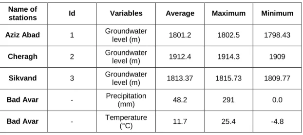
3. Case study and data used
The methods are applied to the data of the Delfan plain, located in the north of the Lorestan Province, Iran. The plain is situated between 47°, 21' and 48°, 21' E to 33°, 48' and 34°, 22' N (see Fig. 3), 1700 to 2100 meters above sea level, in the Zagros mountain chain region. The total area of the plain is about 300 Km2. The high lands of the region are formed by thick layers of limestone and the lowland areas are formed by a combination of igneous, metamorphic, and calcareous structures mixed with metamorphic sheets. The morphological units of the plain consist of different alluvial structures, such as fans and debris. The average annual rainfall in the plains is 480 mm/year. Table 1 presents the features of three observation wells and one meteorological station located in the plain.
Monthly groundwater level (m), precipitation (mm), and temperature (°C) values are used to simulate groundwater level one month ahead. In general, groundwater level responds to the input variables with a delay. Therefore, in the present paper, the input values are considered with time lags. A time lag refers to the value of a variable corresponding to previous months. Table 2 presents different combinations of variables with time lags. In Table 2, Ht, Pt, and Tt refer to the groundwater level, precipitation, and temperature for the present time, respectively. Ht-1, Pt-1, and Tt-1 represent the variable values with one time lag, which means the values of the variables corresponding to the previous month. The observation series are divided into two parts. The first part, including 75% of the series, is used for calibration and the second part, including 25%, is used for validation. In Eq. 5, to produce hybrid models L can take the value of 2. However, to investigate the effect of the decomposition level on simulation, values of L= 1 to 4 are considered in the present paper.
4. Results and Discussion
4.1 Results of GEP model
Different combinations are used for the calibration and validation of the GEP model. Results of the evaluation criteria are presented in Table 3, for the calibration, and Table 4, for the validation.
According to Tables 3 and 4, for well 1, the combination 15 can be selected as the best combination for the GEP model. For combination 15, the R2 is respectively equal to 0.64 and 0.63 for the calibration and validation. For the combination, RMSE and rRMSE are small and the rBIAS value is zero which indicates that the model is unbiased. For well 1, although the R2 of combination 2 is equal to 1 for calibration, the combination is not selected as the best one because its R2 decreases to 0.56 for the validation.
For well 2, GEP shows a weak performance. For calibration, most of the combinations show high R2 values and small RMSE and BIAS, whereas for validation, R2 is low and the combinations indicate large RMSE and BIAS values. For well 2, combination 13 is selected as the best combination.
For well 3, combination 13 is also selected as the best combination because it leads to a high R2 value and zero rBIAS for calibration and has the highest R2 value for validation. According to the results, it is concluded that using variables with time lags produces more accurate results. It is important to mention that the results of the GEP model for combinations 4, 5 and 6, for which only precipitation values are used, is too weak for all observation wells.
4.2 Results of M5 model
To calibrate and validate the M5 model, different combinations described in Table 2 are considered as well. The results of the best combinations for calibration and validation are presented in Tables 5 and 6.
calibration, but it is not selected as the best model because its R2 decreases from 0.80 in calibration to 0.32 for validation, and its RMSE and BIAs increase to 0.62 and -0.18 respectively. For well 1, combinations 10, 11 and 12 are similar to combinations 13, 14 and 15 respectively because the M5 model does not use precipitation values in the simulation. For well 1, M5 leads to a better performance when groundwater level and temperature values are used. On the other hand, the model shows low performances when precipitation values are considered.
For well 2, combination 15 can be selected as the best since it has the largest R2 value for validation. The performance of M5, similarly to GEP, is not good for the groundwater level simulation of well 2. For calibration, M5 shows high R2 and low RMSE and BIAS values, while for validation, the R2 corresponding to all combinations decreases considerably.. For well 2, Similarly to well 1, when only precipitation data are used (combinations 4 to 6) the performance of the model decreases.
For well 3, combination 10 is selected as the best combination because it shows a high performance for both calibration and validation and it leads to similar values of R2, RMSE, rRMSE, BIAS, and rBIAS for calibration and validation. Similarly to wells 1 and 2, when only precipitation data are used for the simulation, the model leads to a lower performance.
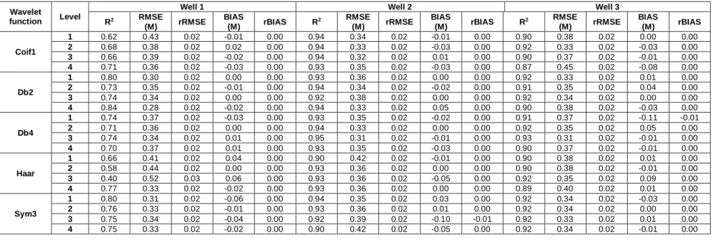
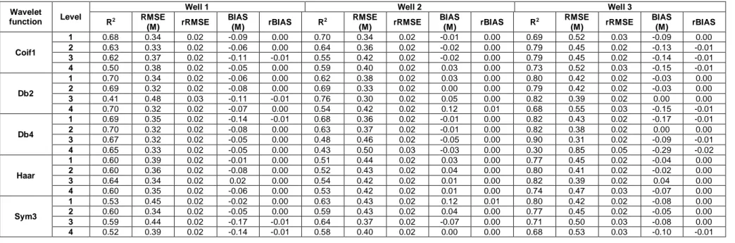
4.3 Results of WGEP model
The results of the evaluation criteria for the WGEP model are shown in Table 7 for calibration, and Table 8 for validation. Results indicate that, for well 1, the mother wavelet of Db4, with L=2, can be selected as the suitable structure for simulation. For well 1, Db2 with L=1 and L=4 also leads to a good performance for validation. However, these combinations are not selected because Db2 with L=4 has an overly complex structure and for Db2 with L=1, the R2 decreases from 0.8 in calibration, to 0.7 in validation, which may indicate that the structure is not good for generalization.
The comparison of Tables 3 and 4 with Tables 7 and 8 shows that using the WT improves the performance of GEP. The improvement is considerable for well 2 in validation. Its R2 increases form 0.4 for the best combination to 0.76 for the best mother wavelet.
4.4 Results of WM5 model
The results of the evaluation criteria for the WM5 model are presented in Table 9 for calibration, and Table 10 for validation. For well 1, the mother wavelets of Coif1 with L=3 and Haar with L=1 show high performances for validation. However, Coif1 with L=3 is selected as the best mother wavelet because its R2 value is higher than Haar with L=1 for calibration. Also, its RMSE, rRMSE, BIAS and rBIAS are smaller than Haar with L=1. For well 2, Db2 with L=4 leads to the best performance. For well 3, all mother wavelets show a good performance. However, the mother wavelet Db2 with L=1 is selected as the best model because the evaluation criteria for both calibration and validation are high and close to each other.
Regarding Tables 9 and 10, it can be concluded that using WT increases the accuracy of M5. Furthermore, it can be concluded that the use of a high level of decomposition does not always lead to an increase in the performance of the models. In a high decomposition level, the sub-signals are too smooth, which means that they do not carry much information. As an example, Fig. 4 presents sub-signals of temperature time series with the mother wavelet of Coif1 with L=8. Fig. 4 shows that when the decomposition level increases, the sub-signals become overly smooth.
4.5 Comparison of different models
Table 11 presents the R2 and RMSE values for the best results of the M5, GEP, WM5 and WGEP models. In the table, rRMSE, BIAS and rBIAS values are not presented because their values are very similar and close or equal to zero.
The performances of M5 and GEP for different combinations indicate that precipitation is not an effective variable for simulation, unlike temperature and groundwater levels. The low effect of precipitation in simulation may be explained by the fact that the case study
during the end of the spring, the whole summer and the beginning of the fall. During these months, groundwater level decreases are observed despite the fact that precipitation is continuously null. Therefore, the M5 and GEP models cannot effectively establish a relationship between precipitation and groundwater level values.
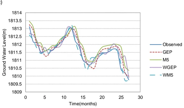
According to Table 11, for all observation wells, hybrid models lead to better performances than simple models. The performances of WGEP and WM5 are close and it is hard to select one of them as the best model. For well 1, the calibration results are close, but for validation, WM5 is a little better than WGEP. For well 2, the validation results of WGEP show a better performance than WM5. Finally, for well 3, WGEP is a little better than WM5 for both calibration and validation, WM5 shows a slightly better performance than WGEP.
The simulated values for the validation are presented in Fig. 5 and compared to the observed values. In Fig. 5, it can be seen that the hybrid models lead to a better fit with observations in comparison with the simple models.
5. Conclusions and future work
The present paper proposes a few methods to simulate groundwater levels. The GEP and M5 models are used for the simulation and WT is used to produce hybrid models, WGEP and WM5. The results indicate that the performances of WGEP and WM5 are close and it is shown that hybrid models are more accurate than the simple ones. However, M5 and WM5 present two advantages. First, the generated models are simpler and more interpretable. It is possible to understand which independent variables have more effect on simulating the dependent variable. Second, running the M5 and WM5 models is faster than running the GEP and WGEP models respectively.
Based on the results of the present work it can be concluded that first, selecting a suitable lag time for input values plays an important role in groundwater level simulation. If a large number of lag times is used, the time for simulation increases, while the lag times are not
the accuracy of hybrid models. A high level of decomposition is not always helpful to increase the accuracy of the model and an optimal decomposition level must also be identified.
Furthermore, it was concluded that temperature and groundwater level values are more effective variables than precipitation values for groundwater level simulation in this arid region of Iran. This means that the selection of hydrological variables as inputs to the models is very specific to the region of study and the climate in question, and it affects significantly the performance of the models. Therefore, it is recommended to carry out exhaustive studies in the future in order to evaluate the effects of other hydrological variables on groundwater simulation and understand the dynamics involved, with the objective of finding suitable variables for groundwater modeling in different climates and conditions.
In the present work, the simulation of groundwater levels was carried out using simple and hybrid models. It would be of interest to evaluate the ability of these models, and other models, for prediction of groundwater levels in 3, 6, and 12 months ahead. This is important as the efficient management of a number of environmental issues (such as droughts) requires a long-term plan.
In the present paper, WT was used to improve the accuracy of the models. It is also suggested, for future studies, to evaluate the effect of using other techniques such as Empirical Mode Decomposition Lee and Ouarda (2011) for, as a tool for pre-processing hydrological time series for groundwater level simulation.
6. Acknowledgements
The presents work was partially supported by the Natural Sciences and Engineering Research Council (NSERC) of Canada.
7. References
[1] Barzegar R, Fijani E, Asghari Moghaddam A, Tziritis E (2017) Forecasting of groundwater level fluctuations using ensemble hybrid multi-wavelet neural network-based models. Science of The Total Environment. 599-600:20-31. doi:https://doi.org/10.1016/j.scitotenv.2017.04.189
[2] Bhattacharya B, Solomatine DP (2005) Neural networks and M5 model trees in modelling water level–discharge relationship. Neurocomputing. 63:381-396. doi:https://doi.org/10.1016/j.neucom.2004.04.016
[3] Bierkens MFP (1998) Modeling water table fluctuations by means of a stochastic differential equation. Water Resources Research. 34:2485-2499. doi:10.1029/98WR02298
[4] Chebana F, Charron C, Ouarda TBMJ, Martel B (2014) Regional Frequency Analysis at Ungauged Sites with the Generalized Additive Model. Journal of Hydrometeorology. 15:2418-2428. doi:10.1175/jhm-d-14-0060.1
[5] Chokmani K, Ouarda TBMJ, Hamilton S, Ghedira MH, Gingras H (2008) Comparison of ice-affected streamflow estimates computed using artificial neural networks and multiple regression techniques. Journal of Hydrology. 349:383-396. doi:https://doi.org/10.1016/j.jhydrol.2007.11.024
[6] Coppola E, Szidarovszky F, Poulton M, Charles E (2003) Artificial Neural Network Approach for Predicting Transient Water Levels in a Multilayered Groundwater System under Variable State, Pumping, and Climate Conditions. Journal of Hydrologic Engineering. 8:348-360. doi:10.1061/(ASCE)1084-0699(2003)8:6(348)
[7] Ebrahimi H, Rajaee T (2017) Simulation of groundwater level variations using wavelet combined with neural network, linear regression and support vector machine. Global and Planetary Change. 148:181-191.