ICEG Conference, 15.-18 November 2015, Al Ain - UAE
Reliability maps for seismic tomography
Thomas Fechner*, Geotomographie GmbH, Neuwied, Germany Solomon Ifeanyi Ehosioke, University of Goettingen, Germany Sonja Mackens, Geotomographie GmbH, Neuwied, Germany Lutz Karl, Geotomographie GmbH, Neuwied, Germany Daryl Tweeton, GeoTom LLC, Apple Valley, Minnesota
Summary
Seismic borehole tomography has become a standard method and is routinely used for the detection of karstic phenomena and the delineation of geological structures. Seismic tomography is believed to be the seismic method promising highest accuracy and reliability. Remaining uncertainties due to a non-zero residual travel time fit during data inversion are often neglected. However, data quality has a significant influence on the accuracy of a travel time pick. We present tomographic inversion results where the signal-to-noise ratio of the first arrival times is considered as a data quality measure during tomographic inversion. This new data quality weighting scheme is supposed to provide more reliable inversion results. Information about the reliability of the tomogram provided along with the seismic tomogram may support the geophysicist interpretation. The effect of the data quality weighted inversion is studied on a field data set.
Introduction
The data quality of seismic signals varies significantly not only from site to site but also within a single data set. Signal quality can range from excellent to poor signal quality. In the case of excellent data quality first arrival time picking is more accurate compared to less reliable arrival time picks for poor signal quality. In general, the accuracy of a first arrival time pick associated with the seismic signal is not considered in the tomographic inversion procedure. Thus, the present tomographic inversion procedures mix travel times of different data quality and reliability and treat them equally weighted. Several authors have described weighting procedures for the well-known tomographic SIRT inversion (Krajewski, C. et al., 1989, Tinti, S. and Ugolini, S., 1990, Lehmann, B., 1992). The proposed weighting procedures consider geometrical properties of the tomographic inversion such as ray density or ray angle azimuth but not signal quality itself. Mackens et al. (2014) proposed the implementation of the data quality weighting using the signal-to-noise ratio of the seismic data and presented first results. This paper presents results obtained during a field campaign in 2014 (Ehosioke, 2014).
Data Quality Weighting
The signal-to-noise ratio influences the accuracy of a first arrival time pick, i.e. the larger the noise the lower the related reliability of the time pick. The signal-to-noise ratio is calculated by the ratio of the maximum first arrival amplitude and the average noise amplitude before the first arrival. This factor is called quality factor (QF) by Mackens et al. (2014) and implemented within the SIRT inversion routine (see equation 1):
(1) with
traveltime residual of ray “k”
length of raypath segment (ray “k”) in voxel “n” index of raypath segments belonging to ray “k” quality factor of ray “k”
slowness residual in voxel “n”
During inversion differences between measured and calculated travel times are weighted with their associated quality factors and finally summed up as weighted slowness corrections. If all quality factors are equal, equation 1 reduces to the well-known SIRT slowness correction for a cell. As a consequence, seismic velocities of rays with higher quality factor will be have greater influence in a model cell than those rays with lower quality factor, i.e., the inverted velocity gets closer to the seismic velocities associated with higher weighted seismic rays. After the final iteration step a mean quality factor in each cell is calculated and can be plotted along with the seismic tomogram velocities. The map of the data quality factors is called reliability map and ranges from “0” to “1”. A reliability map shows areas with low and high quality factors, thus with lower and higher reliability of the seismic velocities. It is recommended to interpret seismic velocities and their associated structures together with their reliability map. Whereas the interpretation of geological structures imaged using the standard inversion procedure cannot differentiate between well resolved and less well resolved structures the new approach allows a more sophisticated interpretation of a tomogram.
Reliability maps for Seismic Tomography
As the reliability map is calculated based on physical measurable values like the signal-to–noise ratio there is a resilient data quality value available and no subjective probability. Thus, the result is reproducible and the interpretation can be well documented. In principle, the data quality weighting used to calculate a reliability map allows any individual data quality criteria to be used during the inversion procedure.
Field Measurement and Data Processing
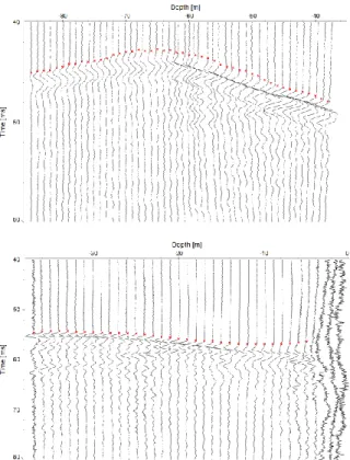
A seismic cross-hole tomography test was carried out in February 2014 at a test site in Hannover to study the heterogeneity of an aquifer. Two boreholes were available to a depth of about 100 m having a distance of approximately 90 m. The geology at the site is characterized by Quaternary fine sand and coarse gravel, underlain by marlstone. Collection of seismic data was carried out using a seismic sparker source type SBS42 from Geotomographie and a hydrophone string type BHC2 with passive sensors type MP25 (Geospace). Sampling interval of the seismograph type DMT Summit was set to 1/16 kHz and shot and receiver spacing was set to one meter.
Figure 1: Seismic example records (shot depth at 75 m for upper record and 16 m for lower record)
Example raw data are shown for two different shot depths at 75 m and 16 m (see figure1). About 3350 first arrival times were picked and the associated quality factors were determined. Statistical analysis on the picking accuracy in respect to data quality showed that a signal-to-noise ratio of 16 can be regarded as sufficient to allow an accurate travel time pick. Thus, an uppermost quality factor threshold of 16 was selected. Values exceeding this threshold were set to 16. After this all quality factors were normalized to 1. Inversion of the travel times was performed using the software GeotomCG (GeoTom LLC). A vertical cell size of 1 m and a horizontal cell size of 2 m were used.
Results and Interpretation
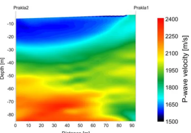
Velocity tomograms were calculated without and with data weighting. Figure 2 shows the seismic velocity tomogram without data weighting.
Figure 2: Seismic velocity tomogram (no data weighting) According to the drilling results seismic velocities below about 1700 m/s belong to unconsolidated aquifer sediments. Velocities above 1700 m/s can be related to weathered to compact marlstone. Figure 3 shows the ray coverage plot for the calculated tomogram. It clearly shows highest ray coverage in the middle of the tomogram and lower ray coverage at top and bottom.
The ray coverage map as shown in figure 3 is typically used to conclude that highest confidence can be given to the center of the seismic tomogram as there is the highest density of ray paths. Anyhow, by introducing the data weighting into the inversion a somewhat different conclusion can be drawn.
Reliability maps for Seismic Tomography
Figure 3: Ray coverage for seismic tomogram (no data weighting)
Figure 4 shows the map of the data quality obtained after inversion of the same data set introducing quality factors. This map is called reliability map and shows the distribution of the averaged data quality factors for each tomogram cell. Data quality values close to one can be related to an excellent reliability of the seismic velocity estimation whereas low data quality values are associated with a poor velocity estimate.
Figure 4: Reliability map of data quality factors (data weighting)
The reliability map presented in figure 4 shows higher quality factors in the upper part of the map. The lower and the center part show medium data quality values. This result allows a different interpretation of the seismic tomogram obtained using weighted data quality factors shown in figure 5.
Figure 5: Seismic velocity tomogram (data weighting) After this the seismic velocities within the unconsolidated sediments are well determined thus the basin like structure of lower seismic velocities is well resolved and can be trusted. An interpretation based on ray coverage only would most likely lead to a conclusion that this structure might be related to the low ray coverage itself shown in figure 3. Lower data qualities are imaged in the lower right corner of the seismic tomogram and associated with the low seismic velocities of the marlstone. Obviously, the marlstone is strongly weathered in this area. Anyhow, according to the reliability map the velocity contours are not as reliable as in other parts of the tomogram. This is also in agreement with the map of the slowness residual error left after the final iteration due to a non-perfect travel time fit between measured and calculated travel times (see figure 6). This map shows the slowness residual s normalized by the slowness s of a cell. Areas with relative slowness residual errors close to 0 indicate good estimates of the local seismic velocity. Negative or positive relative slowness residual errors are a sign of underestimated or overestimated velocities, respectively.
Figure 6: Map of the relative slowness residual error (data weighting)
Reliability maps for Seismic Tomography
Conclusions
Reliability map calculation based on a data quality weighted seismic travel time inversion scheme has been presented. The reliability maps are meant to support the interpretation by geophysical engineers. Up to now velocity structures visible in tomograms are only supported by the interpretation of the ray coverage. Using the reliability map and quality factor values areas of higher or lower reliability of the seismic velocity can be documented. Additionally, the plot of the remaining relative slowness residual errors calculated after the final iteration provides helpful information about the reliability of a tomogram.
References
Ehosioke, S., 2014, Application of Cross-Hole Seismic Tomography in Characterization of Heterogeneous Aquifers, University of Goettingen, Germany, Master Thesis.
Krajewski, C., Dresen, L., Gelbke, Ch., and Rueter, H., 1989, Iterative Tomographic Methods to Locate Seismic Low-Velocity Anomalies: A Model Study, Geophysical Prospecting 37, Issue 7, P. 717-751.
Lehmann, B., 1992, Modellseismische Untersuchungen zur Transmissions- und Reflexionstomographie unter Verwendung der Gauß-Beam Methode, Phd-Thesis, Ruhr-University Bochum, Reihe A, Nr. 33 (in German).
Lehmann, B., 2007, Seismic Traveltime Tomography for Engineering and Exploration Applications, EAGE publications bv, DB Houten, The Netherlands, P. 37-57 Mackens, S., Karl, L., Fechner, Th. and Tweeton, D., 2014, Interpretation of Seismic Tomography Results Using Data Quality and Residual Error Maps, FastTimes, June 2014, Volume 19, Number 2.
Tinti, S. and Ugolini, S., 1990, Pre-Selection of Seismic Rays As a Possible Method to Improve the Inverse Problem Solution, Geophysical Journal International 102, Issue 1, P. 45-61.