AND
ASTROPHYSICS
Detection of the lensing galaxy in HE 1104-1805
?
F. Courbin1,2, C. Lidman3, and P. Magain1?? 1
Institut d’Astrophysique, Universit´e de Li`ege, Avenue de Cointe 5, B-4000 Li`ege, Belgium
2 URA 173 CNRS-DAEC, Observatoire de Paris, F-92195 Meudon Principal C´edex, France 3
European Southern Observatory, Casilla 19001, Santiago 19, Chile Received 17 July 1997 / Accepted 17 September 1997
Abstract. We report on deep IR imaging of the double quasar HE 1104–1805. A new image deconvolution technique has been applied to the data in order to optimally combine the numerous frames obtained. The resulting J and K0
images allow us to de-tect and study the lensing galaxy between the two lensed QSO images. The near infrared images not only confirm the lensed nature of this double quasar, but also support the previous red-shift estimate of z = 1.66 for the lensing galaxy. No obvious overdensity of galaxies is detected in the immediate region sur-rounding the lens, down to limiting magnitudes of J = 22 and K = 20. The geometry of the system, together with the time delays expected for this lensed quasar, make HE 1104–1805 a remarkable target for future photometric monitoring programs, for the study of microlensing and for the determination of the cosmological parameters in the IR and optical domains.
Key words: gravitational lensing – quasars: HE 1104–1805 – methods: data analysis
1. Introduction
It is well established that gravitationally lensed quasars are unique natural rulers for measuring the Universe and for deriv-ing the cosmological parameters (Refsdal, 1964a,b). Measurderiv-ing the time delay from the images of a lensed QSO can provide an estimate of the Hubble parameter H0, independent of any other
classical method. However, a good knowledge of the geometry of the lensed system is mandatory for the method to be effective (e.g. Schechter et al, 1997; Keeton & Kochanek, 1996; Courbin et al, 1997). In spite of this crucial requirement and although the number of known gravitationally lensed quasars does not stop increasing (see for a review Keeton & Kochanek, 1996), the pre-cise geometry of most lensed QSOs remains poorly known. In most cases, even the matter responsible for the lensing, whether
Send offprint requests to: F. Courbin (Li`ege address)
?
Based on observations obtained at ESO, La Silla, Chile
??
Also Maˆıtre de Recherches au FNRS (Belgium)
it be in the form of a single galaxy or several galaxies, is not detected. The high redshifts of these galaxies (hence their faint apparent magnitudes) and the strong blending with the nearby much brighter QSO images are the main reasons for their non-detection.
Imaging in the near IR (1 to 2.5 microns) has the advantage that the relative brightness between the lensed QSO and any lensing galaxy decreases, making the galaxy easier to detect. The disadvantage is that the IR sky is considerably brighter. This forces one to take many images to avoid detector saturation; however, this turns out to be an advantage (see Section 3).
This paper presents IR observations of the quasar HE 1104– 1805. The strong similarity between the optical spectra obtained for its two components (Wisotzki et al, 1993) makes HE 1104– 1805 a good gravitational lens candidate. The high redshift of the object (z = 2.316, Smette et al, 1995) and the relatively wide angular separation between the lensed images (3.200
) indicate that a large mass is involved in the lensing potential. If the deflector is a high redshift galaxy or a galaxy cluster, deep IR observations should reveal it.
We used a recently developed image deconvolution algo-rithm (Magain, Courbin & Sohy, 1997; hereafter MCS) to opti-mally combine the numerous IR frames and obtain deep, sharp images of HE 1104–1805. The present paper describes how this powerful technique allows us to study the immediate environ-ment of HE 1104–1805 and detect the lensing galaxy.
2. Observations-reductions
The observations took place at the ESO/MPI 2.2m telescope situated at La Silla Observatory, Chile, on the nights of April 14 and 15, 1997. The IR camera IRAC2b was used at the Cassegrain focus of the telescope. The detector of IRAC2b is a 256×256 NICMOS 3 HgCdTe array and the instrument has a variety of optical lenses available for imaging at different pixel scales. Lens LB (Lidman, Gredel & Moneti, 1997) was chosen since it gives a good compromise between the pixel scale (a small pixel is needed for the deconvolution) and the size of the field. During the observations, PG 1115+080 was also observed. A by-product of these observations is a more accurate estimate of
58 F. Courbin et al.: The lensing galaxy in HE 1104-1805
the IRAC2b pixel size for images taken in lens LB. The new scale, 0.276200/pixel, is based on the precise astrometry of this
field given by Courbin et al. (1997). This results in a field of view of 7100
.
Numerous short exposures of HE 1104–1805 were obtained in J (λc=1.25 micron) and K0 (λc=2.15 micron) under good
meteorological conditions. The mean seeing was 0.007-0.008 and
the sky was photometric. We set the Detector Integration Time (DIT) to 20 sec in K0
and 60 sec in J . Each image taken in K0
(resp. J ) is the average of 3 (resp. 2) such integrations. The choice of the DIT is dictated by detector saturation. The number of DITs is dictated by the frequency at which the sky intensity varies. Since the field of HE 1104–1805 is uncrowded, we took sequences of 9 science exposures, dithered in a random manner by 5 to 1000
, always keeping the object and three PSF stars in the field.
Dome flat-fields were taken in order to correct for the pixel to pixel sensitivity variations of the detector. However, dome flat-fields do not accurately represent the large scale sensitivity variations of the array, in the J band. Fortunately, this variation does not show strong gradients and has a maximum amplitude of 3-4% over the whole field. It was modeled by observing a bright star over a grid of 9 different positions across the array and by fitting a two dimensional, third order polynomial to the flux of the star. The residuals of the fit were 1%. This fit, which is commonly called an illumination correction, was multiplied by the dome flat to produce the final flat-field containing both the low and high frequency sensitivity variations of the array. After subtraction of a dark frame, the flat-field correction is applied to all scientific frames.
The background is removed from every exposure. It is esti-mated for any particular exposure by averaging the 6 preceding and the 6 following exposures. Thanks to the dithering between exposures, objects in these frames could be rejected before the average was taken. This method allows us to accurately follow the background which varies on the time scale of a few minutes. Standard stars were observed every two hours. The standard deviation in the zero points were 0.024 magnitudes in J and 0.012 magnitudes in K. The magnitude and colours in this paper are in the J HK system as defined by Bessell and Brett (1988).
3. Image combining/deconvolution
The frames were combined in two ways. First, the standard reduction and image combination techniques implemented in the IRAF package were used in order to average the frames. The sigma-clipping algorithm was used for bad pixel rejection. This leads to two deep J and K0
images over a field of 10
. The total exposure times were 5040 sec in J and 8100 sec in K0
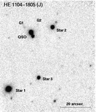
. The resulting detection limit is 22 in J and 20 in K (3σ, integrated over the whole object). Fig. 1 presents the field in the J band.
Fig. 1. A field of one arc-minute around HE 1104–1805. The detection limit on this deep J band image is 22. West is to the top, North to the left. The PSF stars are labeled. No obvious galaxy overdensity near the QSO pair can be seen; only galaxies G1 and/or G2 might be involved in the lensing potential.
3.1. Image deconvolution
In order to study the immediate environment of HE 1104–1805, we used the new MCS deconvolution algorithm described in full detail by Magain, Courbin & Sohy (1997).
Deconvolution of an image by the total observed Point-Spread-Function (PSF) leads to the so-called “deconvolution artifacts” or “ringing effect” around the point sources. This re-sults from the deconvolution algorithm attempting to recover spatial frequencies higher than the Nyquist frequency, thus vi-olating the sampling theorem. Instead, the MCS algorithm uses a narrower PSF which ensures that the deconvolved image will not violate the sampling theorem. Additionally, the MCS algo-rithm takes advantage of important prior knowledge: in the de-convolved images, all the point sources have the same (known) shape. This allows us to decompose the deconvolved image into a sum of analytical point sources plus a diffuse background which is smoothed to the final resolution chosen by the user. Most of the deconvolution artifacts are thus avoided. This is of particular interest when one wishes, like in the present study, to discover faint objects embedded in the seeing disks of much brighter point sources.
If the deconvolution of a single image already yields very good results (e.g. Courbin et al. 1997), the simultaneous decon-volution of numerous dithered exposures is even more efficient
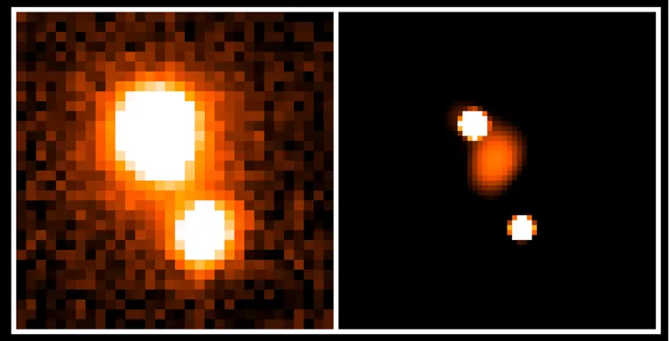
Fig. 2. Left: A J band image of HE 1104–1805 obtained with 2.2m ESO/MPI telescope. The field is 8.800and the total exposure time is 5040 sec.
Right: Simultaneous deconvolution of the 6 intermediate images (see text). The adopted pixel size is 0.001381. The FWHM of the point sources
on the deconvolved image is 0.002762.
(e.g. Courbin & Claeskens, 1997). In particular, the MCS code allows the pixel size of the deconvolved image to be as small as desired. This over-sampling possibility, already applicable to the deconvolution of a single frame, is of considerable interest when dealing with the spatial information contained in many dithered frames.
Another advantage of the MCS algorithm is that the PSF can vary from frame to frame. For example, one can combine good quality images with trailed or even defocused images or, in a more reasonable way, frames of differing image quality and signal-to-noise ratios. The resulting frame is an optimal combination of the whole data set, with improved resolution and sampling.
The seeing in the original IRAC2b images was of the order of 0.00
6 for the very best frames and up to 1.00
2 for the worse ones, in both J and K0
. We adopted for the deconvolution a sampling step of 0.00
1381, two times smaller than the original pixel size. This allows us to reach a final resolution of 0.00
2762 which still samples well the resulting image (2 pixels Full-Width-Half-Maximum (FWHM)).
Since the signal-to-noise of individual images is very low and since we had to reject very numerous bad pixels, we first combined the images in groups of nine. Thus, we obtained 6 intermediate images in J and 12 images in K0
. A PSF was derived for each of these images. In K0
, only “Star 1” is bright enough, - i.e. comparable to the QSO’s luminosity - to compute an accurate PSF (See Fig. 1 for the labeling of the stars used). In J , “Star 1” shows extended luminosity so we used both “Star 2”
and “Star 3”. The resulting total exposure time of the co-added images is different from the one of the images combined using IRAF and the standard methods. We rejected more frames with bad pixels falling right on the object or the PSF stars. On the other hand, we included in the different stacks more images with bad seeing. Thus, the total exposure time of the deconvolved images is 6480s in both J and K0
.
The program requires initial estimates for the positions and intensities of the point sources in the field. This was done by choosing the central pixel of each QSO image. During decon-volution, the centres of the point sources are forced to be the same in all the images, only an image translation (no rotation) being allowed. The data are never aligned or rebinned; only the deconvolved model (on which the highest spatial frequencies are modeled analytically) is transformed. The intensities of the point sources can be allowed to be different in each image so that even variable objects may be considered in the deconvolution.
The shape of IRAC2b PSF shows significant variations across the field. In J , the variation is still acceptable, mainly because we used “Star 2” and “Star 3”, which are closer to HE 1104–1805 than “Star 1”, which is used for the PSF com-putation in the K0
band. It is possible in our algorithm to let the PSF depart slightly from its original shape, during the deconvo-lution process. It is in fact re-determined directly from the point sources in the field that is deconvolved. In the present case of simultaneous deconvolution, the correction on the PSFs is well constrained by the numerous images considered. The quality of the PSF correction is even better if numerous stars are present
60 F. Courbin et al.: The lensing galaxy in HE 1104-1805
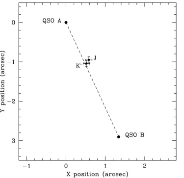
Fig. 3. Geometry of HE 1104–1805. Note the slight misalignment be-tween the 2 QSOs and the lensing galaxy.
in the field. With 2 point sources and 12 images in K0
, it has been possible to correct rather well the PSFs of the 12 images. The deconvolution is first performed with variable PSFs, and then repeated with the corrected PSFs fixed.
The background component of the deconvolution is smoothed on the length scale of the final resolution. The weight attributed to the smoothing (see Magain, Courbin & Sohy, 1997 for more detail) is chosen so that the residual map between each data frame and the model image (reconvolved with the PSF) in units of the photon noise, has the correct statistical distribu-tion, i.e. is equal to unity all over the field. In other words, we chose the smoothing term by inspecting the local residual maps. This ensures that the deconvolved image is compatible with the whole data set in any region of any of the data frames.
The deconvolution consists of a χ2 minimization between the deconvolved model image and the whole data set, using an algorithm derived from the conjugate gradient method. Again, the residual maps are used as a quality check of the result. We stop the iteration process only when the residual maps show the correct statistical distribution all over the field so that we avoid local over or under-fitting.
The program produces the following outputs: a deconvolved image, the centre of the point sources, the shifts between the images, the intensities of the point sources for each of the indi-vidual frames and an image of the deconvolved galaxy, free of any contamination by the QSOs.
3.2. Results
Fig. 2 displays the result of the deconvolution for the J band images. Six images were used to obtain this result. The spatial
Table 1. Summary of the astrometry (in the same orientation as Fig. 1 and Fig. 2) and photometry for HE 1104–1805 and the lensing galaxy. The 1σ error bars are also indicated.
QSO A QSO B Lens
J 15.94 ± 0.06 17.47 ± 0.08 19.01 ± 0.2 K 14.78 ± 0.08 16.13 ± 0.11 17.08 ± 0.2 J − K 1.16 ± 0.09 1.34 ± 0.13 1.93 ± 0.3 x (00) 0.00 ± 0.03 +1.34 ± 0.03 +0.55 ± 0.05
y (00) 0.00 ± 0.03 −2.90 ± 0.03 −1.00 ± 0.05
Table 2. Astrometry and photometry of galaxies G1 and G2, relative to QSO A. The astrometry is given in the same orientation as Fig. 1 and Fig. 2. These values were derived from the “un-deconvolved” images.
G1 G2 J 20.3 ± 0.3 21.4 ± 0.4 K 19.2 ± 0.3 19.7 ± 0.5 J − K 1.1 ± 0.4 1.7 ± 0.6 x (00) −4.7 ± 0.1 +4.2 ± 0.1 y (00) +3.1 ± 0.1 +5.0 ± 0.1
resolution is 0.002762, comparable to the resolution reached by
the HST in the IR domain. We chose the same final resolution for the simultaneous deconvolution of 12 K0
images. The lensing galaxy is clearly detected and displayed in Fig. 2. It is also seen in K0
, were it is in fact brighter.
The images were deconvolved several times, with different initial guesses as to the position and the intensity of the QSO pair. In Table 1 the relative positions of the QSOs are tabulated. The errors correspond to the dispersion in the different decon-volutions (1σ error bars).
The photometry of the QSO images is also given. The 1σ errors correspond to the dispersion in the peak intensities in each of the images considered in the simultaneous deconvolution (6 in J , 12 in K0).
The position of the lensing galaxy was determined on the de-convolved background image by both Gaussian fitting and first order moment calculation. The results were averaged together and taken as the position of the lensing galaxy. We estimate the 1σ error on the galaxy position to be about 0.00
08 in both bands. The values given in Table 1 are the average of the positions in J and K0
and have an estimated error of 0.00
05. The angular separation between the lensing galaxy and QSO A is 1.1400
± 0.0600
and the distance between the two QSO images is 3.1400
± 0.0400.
We derived the magnitude of the lensing galaxy by aper-ture photometry on the deconvolved background image to avoid contamination by the QSO’s light. A diaphragm of 0.009 diameter
was used. Due to the too low signal-to-noise ratio in the lensing galaxy, we could not determine its shape parameters.
Fig. 3 shows the position of the galaxy, relative to the QSO images. A slight misalignment between the lens and the line joining QSO A and QSO B can be seen. It is larger than our error bars and is apparent in both J and K0
. In addition, the PSF’s shape does not show any significant variations across the deconvolved field (only 8.800
Fig. 4. J − K as a function of redshift for different galaxy types (see Sect. 4 for more details). The shaded region shows the colour of the lensing galaxy, error bars included. The thick lines show the models which take into account galaxy evolution; the thin lines do not. A solid arrow shows the redshift of the QSO pair. The two strongest metal absorption line systems, at redshifts z = 1.320 and z = 1.6616, are marked with dotted arrows.
can be ruled out. The observed misalignment seems therefore real.
No obvious galaxy overdensity is detected in the immediate surrounds of the QSO, although the detection limit of 22 in J and 20 in K would have allowed us to see any rich cluster up to z = 2. The two nearest objects to the double QSO are galaxies G1 and G2 (see Fig. 1). Table 2 gives their position relative to QSO A and their photometry, both derived on the “un-deconvolved” image since they are outside the field used for the deconvolution.
4. Colour of the deflector
The redshift of the lensing galaxy can be constrained by the J − K colour. In Fig. 4, we compare the colour of the candidate (the shaded region) with theoretical colours corresponding to five galaxy types. These colours were obtained from the PEGASE ”Projet d’Etude des GAlaxies par Synth`ese Evolutive” atlas (Leitherer et al. 1996; Fioc and Rocca-Volmerange 1997). The five types correspond to E, Sa, Sb, Sc and Sd galaxies in a critical density universe with H0 = 50 (Rocca-Volmerange and
Fioc 1996). The theoretical colours are a function of redshift. The thick lines include the effect of galaxy evolution; the thin lines do not.
The colour of the candidate constrains the object to be a galaxy with a redshift beyond z = 0.4, probably between z=1 and z=2. The redshifts of the two strongest metal absorption line
Elliptical Sa
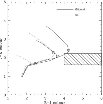
Fig. 5. A R − J vs. J − K colour-colour plot showing the tracks from z = 0 to z = 2.5 of two galaxy types, an elliptical and a spiral. The thick lines correspond to the models which take into account galaxy evolution. The location of a galaxy at z = 1.66 is marked by the circles. Also plotted are the limits derived from Wisotzki et al. (1993) and this paper.
systems, at z = 1.320 and z = 1.6616 (Smette et al. 1995 and Wisotzki et al. 1993) are marked with dotted arrows in Fig. 4.
Without a firm redshift for the lens, its absolute magnitude is unknown. However, if the galaxy is between z = 1 and z = 2 (as also suggested by Smette et al. 1995) it is many times more luminous than a typical large galaxy, which would have M?
K =
−24.75. This value we adopted for M?
Kis the average between
the value determined by Glazebrook et al. (1995) and the one from Mobasher et al. (1993).
5. Discussion-conclusions
The main result of the present study is the detection of a red fuzzy object located between the two components of HE 1104– 1805. This result is one more very strong argument in favour of the lensed nature of this double quasar.
Wisotzki et al (1993) do not detect the lensing galaxy in R down to a limiting magnitude of 23-24. In Fig. 6 the tracks in the R − J vs J − K colour-colour diagramme of two galaxy types, an elliptical and an Sa galaxy, are plotted. They are plotted with and without evolution and for the redshift range 0 < z < 2.5. Also plotted is the range allowed by the observations in this paper and the optical observations of Wisotzki et al. (1993).
If we include the effects of evolution (thick lines in the fig-ures), the IR colours are compatible with an elliptical galaxy (as shown by Fig. 5) between z = 1 and z = 2 (Fig. 4). The IR-optical colours are less compatible with this; however, the
62 F. Courbin et al.: The lensing galaxy in HE 1104-1805
expected R magnitude of the lensing galaxy is R = 22.5, and this may have been difficult to see 1.001 away from the QSO which is
5 to 6 magnitudes brighter. In fact, a preliminary detection of the lensing galaxy by Grundahl, Hjorth & Sørensen (1995) allowed to measure an I-band magnitude of 20.6, in better agreement with our findings.
One of the two metallic absorption line systems found at z = 1.320 and z = 1.6616 (Smette et al. 1995) could be produced by the lensing galaxy. In particular, the absorption system at z = 1.6616 is seen almost only in QSO A. Since the angular distance from the lens to QSO A is much smaller than to QSO B it seems reasonable to think that the lensing galaxy we detect is more likely to be at z = 1.6616 rather than 1.320.
Despite the depth of our IR images, which enables us to detect M?
Kgalaxies up to the redshift of the QSO, we do not
de-tect any obvious overdensity of galaxies which could contribute significantly to the total gravitational potential involved in this system. However, two faint galaxies (G1 and G2) are detected close to the line of sight to the QSO. G1 has a J − K colour of 1.1, while G2 has a colour close to that of the lens galaxy. These two objects could constitute an external source of shear, for example responsible for the misalignment between the lens-ing galaxy, QSO A and QSO B. However, one cannot exclude the simpler (but unlikely) explanation that the light and mass centroids of the lensing galaxy do not coincide.
We can infer from our deconvolutions that QSO A is not ex-actly compatible with a single point source. The deconvolution leaves significant residuals at the location of QSO A, even in J where the PSF is rather stable across the field. The signal-to-noise ratio and resolution of our observations do not allow to draw definite conclusions, but we suspect that image A is either not single or is super-imposed on a fuzzy faint light distribution. From the geometry of the lensed system, given in Table 1, and assuming we see a galaxy at z = 1.6616, the time delay we can expect between the two images of HE 1104–1805 is of the order of 3.5 years. We have assumed that the lens can be modeled as a Singular Isothermal Sphere (SIS) and that H0 = 50
km s−1Mpc−1. This large delay means that one measurement every second week would be enough to derive good light curves. Assuming that an SIS is appropriate for the lensing galaxy, we derive a mass of 7·1011M , not too far above the masses
ex-pected for big elliptical galaxies. The apparent magnitude sug-gests that the lens is many times more luminous than a normal galaxy if the lens is actually at z = 1.66.
Finally, the magnitude difference between the lensed images is∆J = 1.53 ± 0.1 and ∆K = 1.35 ± 0.1, where the magni-tude difference is taken as mag(QSO B)−mag(QSO A). The magnitude difference expected from the SIS model is 0.75 mag-nitude, but with the deflector angularly closer to the faint image than to the brighter one.
This could indicate that component B is reddened relative to A, or that component A is preferentially amplified (e.g. slight image splitting) relative to B and that this preferential amplifi-cation is more efficient in the blue. The latter hypothesis is more likely since the lens galaxy is angularly closer to QSO A than to QSO B and would therefore redden A more than B,
assum-ing the reddenassum-ing is due to the lens galaxy. On the other hand, the lensing potential might be more complex than a SIS (for example elliptical + core), in particular if G1 and G2 introduce a significant source of shear.
Wisotzki et al. (1995) showed that microlensing was acting on QSO A and that it was more efficient in the blue than in the red. The magnitude difference they observed in B in 1994 was∆B = 1.85, larger than our present values in J and K (al-though the quasar has probably varied between 1994 November and 1997 April). This suggests that microlensing is less effi-cient in the IR than in the visible. If the source quasar is found to be variable in the IR domain, an IR photometric monitoring of HE 1104–1805 may then minimize contamination by mi-crolensing events and allow a better determination of the time delay than with optical data.
Acknowledgements. The authors would like to thank J.-P. Swings, P. Schechter, J. Hjorth and the referee Y. Mellier for helpful com-ments on the first version of this manuscript. This work has been in part financially supported by the contract ARC 94/99-178 “Action de Recherche Concert´ee de la Communaut´e Franc¸aise” (Belgium), and Pˆole d’Attraction Interuniversitaire P4/05 (SSTC, Belgium).
References
Bessell M. S. and Brett J. M. 1988, PASP 100, 1134 Courbin F., Claeskens J.-F., 1997, ESO messenger 88, p 32 Courbin F., Magain P. Keeton C.R., et al, 1997, A&A 324, L1 Fioc M., and Rocca-Volmerange B., 1997, A&A, in press
Glazebrook K., Peacock, J. A., Miller, L. and Collins, C. A. 1995, MNRAS, 275, 169.
Grundahl F., Hjorth J., Sørensen A.N., 1995, in “Highlights of Astron-omy”, Vol. 10 (Kluwer) Dordrecht, 658-659, Appenzeler I. (ed.) Keeton C.R., Kochanek C.S., 1997, ApJ 487, 42
Keeton C.R., Kochanek C.S., 1996, Proceedings of the 173rd IAU Symposium: “Astrophysical Applications of Gravitational Lens-ing”, Melbourne, Australia, eds. Hewitt and Kochanek (Kluwer), p 419.
Lidman C., Gredel R., Moneti A., 1997, “ESO-IRAC2b user manual” Lietherer et al. 1996, PASP 108, 996.
Magain P., Courbin F., Sohy S., 1997, ApJ, in press, preprint astro-ph/9704059
Mobasher B., Ellis R. S. and Sharples R. M. 1993, MNRAS 263, 560. Refsdal S., 1964a, MNRAS 128, 295
Refsdal S., 1964b, MNRAS 128, 307
Rocca-Volmerange B., and Fioc M., 1997, in preparation Schechter P.L. et al. 1997, ApJ 475, L85
Smette A., Robertson J. G., Shaver P. A., Reimers D., Wisotzki L., and K¨ohler T. 1995, A&ASS 113, 199.
Wisotzki L., K¨ohler T., Kayser R., Reimers D., 1993, A&A 278, L15 Wisotzki L., K¨ohler T., Ikonomou M., Reimers D., 1995, A&A 297,
L59
This article was processed by the author using Springer-Verlag LaTEX A&A style file L-AA version 3.