Subspace and nonlinear-normal-modes-based identification of a beam
with softening-hardening behaviour
C. Grappasonni, J.P. No ¨el, G. Kerschen
Space Structures and Systems Laboratory (S3L) Department of Aerospace and Mechanical EngineeringUniversity of Li `ege, Li `ege, Belgium chiara.grappasonni, jp.noel, g.kerschen@ulg.ac.be
ABSTRACT
The capability to reproduce and predict with high accuracy the behaviour of a real system is a fundamental task of numerical models. In nonlinear structural dynamics, additional parameters compared to classical linear modelling, which include the nonlinear coefficient and the mathematical form of the nonlinearity, need to be identified to bring the numerical predictions in good agreement with the experimental observations. In this context, the present paper presents a method for the identification of an experimental cantilever beam with a geometrically nonlinear thin beam clamped with a prestress, hence giving rise to a softening-hardening nonlinearity. A novel nonlinear subspace identification method formulated in the frequency domain is first exploited to estimate the nonlinear parameters of the real structure together with the underlying linear system directly from the experimental tests. Then a finite element model, built from the estimated parameters, is used to compute the backbone of the first nonlinear normal mode motion. These numerical evaluations are compared to a nonlinear normal modes-based identification of the structure using system responses to stepped sine excitation at different forcing levels.
Keywords: Nonlinear system identification; subspace identification; experimental test; softening hardening behaviour; nonlinear
normal modes.
1 INTRODUCTION
The physical behaviour of a structure undergoing high energy vibrational regimes can represent a challenging problem even in the case of simple one-dimensional flexible structures. When investigated using linear system identification techniques, the dynamical phenomena can be erroneously interpreted and lead to an inaccurate model. This results in the inapplicability of traditional, well-established linear techniques that needs to be reformulated in order to include the (predominant) nonlinearities in the measuring, identification and modelling processes. Several techniques are available today for the experimental identification of the linear structure dynamics and they can be classified as Phase Resonance or Phase Separation methods, depending on the sequential or simultaneous excitation of the normal modes, respectively. In the first case an accurate estimate of each mode is achieved by means of resonance excitation and concurrent response measuring. On the other hand, when a band-limited signal is used to vibrate the structure in the whole band of interest, the Frequency Response Functions (FRFs) between the system outputs and inputs can be evaluated and one of the many available modal analysis algorithms can be applied to assess the modal parameters. Starting from the sophisticated and advanced subspace-based algorithms[1, 2] the frequency-domain nonlinear subspace identification (FNSI) method has been developed and successfully applied to nonlinear structures[3]. The FRFs of the underlying linear structure and the nonlinear restoring force law can be estimated by this approach starting from the measurements of both the system responses and excitations. Therefore, the modal parameters, such as the natural frequencies, the damping ratios and the mode shapes, and the nonlinear coefficients can be estimated and used to implement an accurate
model of the structure under investigation. The robustness of such a model allows its use to predict the structure behaviour to other excitations than the one used for the identification process. Moreover a high-fidelity model can exhibit extremely interesting and complex phenomena characterizing nonlinear structures, such as bifurcations, internal resonances, modal interactions and others[4].
Nonlinear normal modes (NNMs) offer a solid theoretical and mathematical tool for interpreting a wide class of nonlinear dynami-cal phenomena, yet they have a clear and simple conceptual relation to the classidynami-cal linear normal modes (LNMs). The relevance of the NNMs for the structural dynamicist is addressed in [5] and their practical computation using numerical continuation tech-niques is explained in [6]. An experimental evaluation of the NNM motions is also possible and its rigorous implementation starting from the Phase Resonance method for linear structures has been derived and validated in [7]. The stepped sine ex-citation provided by a shaker can be used to achieve a forced response of the structure in nonlinear regimes and from the simultaneous measurement of the harmonic loading and responses the NNM motion can be extracted.
In this context, the objective of the present paper is to address the identification of a cantilever beam connected at its free-end to a thin, short beam that exhibits a combined softening-hardening nonlinearity. This set-up was proposed in [8]. It is slightly modified in the present study in the sense that the two beams were manufactured as a single piece (i.e., a monolithic set-up) to avoid bolting the two beams at their intersection. Due to residual stresses produced by the manufacturing process, the thin beam is slightly curved at rest. Its clamping therefore generates a prestress which was found to give rise to softening nonlinearity for low excitation levels. Conversely, the high flexibility of the thin beam introduces a hardening geometrical nonlinearity when large deflections occur. Random FNSI FRF underlying linear system Nonlinear restoring force M, C, K model updating Continuation Backbone Backbone
Sine Phase Resonance
NNMs
Comparison
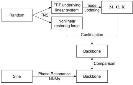
Figure 1: Diagram of the system identification methodology as addressed in the present study.
The proposed methodology is summarised in Figure 1. Starting from measured data from band-limited periodic random excita-tion, the FNSI method is applied where the restoring force is modelled using splines for increased flexibility. Structural matrices
M, C and K are updated from the FRFs of the underlying linear system using classical linear model updating. Then a numerical continuation algorithm is used to derive the backbone of the first mode (i.e., the locus of the resonance peaks). The same back-bone is also identified experimentally combining stepped sine excitation and a nonlinear generalization of the Phase Resonance method . This approach allows for a direct correlation between the two backbones.
The present paper is organised as follows. In the next section, the FNSI method is introduced. In Section 3 the definition of NNMs is briefly recalled together with the description of their energy dependence. Their numerical computation and experimental evaluation are also addressed. Section 4 explains the test case with the softening-hardening nonlinearity and it describes the experimental setup. In Section 5 the results from FNSI are described as they give the parameters for the implementation of the numerical nonlinear model. Finally in Section 6, the NNM-based system identification is carried out and a comparison with the numerical achievements from a continuation toolbox is performed.
2 SUBSPACE IDENTIFICATION OF NONLINEAR MECHANICAL SYSTEMS IN THE FREQUENCY DOMAIN
The FNSI method is a subspace identification algorithm dedicated to mechanical system models incorporating linear-in-the-parameters nonlinearities[3]. Linearity in the parameters avoids an iterative optimisation process, and issues related to initial-isation and convergence thereof. The technique exploits data in the frequency domain which are more compact than in the time domain. The frequency domain also offers convenient insights into the impact of nonlinearities on the system’s dynamics. The FNSI method is naturally a multi-input, multi-output identification scheme as it constructs state-space models of nonlin-ear mechanical systems. Its implementation relies on robust tools from numerical analysis, including QR and singular value decompositions.
2.1 Nonlinear model equations in the physical space
The vibrations of nonlinear mechanical systems possessing an underlying linear regime of motion are governed by the time-continuous model
M ¨q(t) + Cvq(t) + K q(t) + g(q(t), ˙˙ q(t)) = p(t) (1)
where M, Cv, K ∈ Rnp×npare the linear mass, viscous damping and stiffness matrices, respectively; q(t) and p(t) ∈ Rnp
are the generalised displacement and external force vectors, respectively; g(t)∈ Rnpis the nonlinear restoring vector
encom-passing elastic and dissipative effects, and npis the number of degrees of freedom (DOFs) of the structure obtained after spatial
discretisation. The amplitude, direction, location and frequency content of the excitation p(t) determine in which regime the structure behaves.
The effects of the r lumped nonlinear components in the system are represented using a linear-in-the-parameters model of the form g(q(t), ˙q(t)) = r ∑ a=1 sa ∑ b=1 ca,bha,b(q(t), ˙q(t)). (2)
In this double sum, sa is the number of nonlinear basis functions ha,b(q(t), ˙q(t)) selected to describe the a-th nonlinearity,
and ca,b are the associated coefficients. The total number of nonlinear basis functions introduced in the model is equal to
s = ∑ra=1sa. Given input-output measurements of p(t) and q(t) or its derivatives, and an appropriate user selection of the
functionals ha,b(t), the FNSI method aims at deriving estimates of the modal properties of M, Cvand K and of the nonlinear
coefficients ca,b.
2.2 Feedback interpretation of nonlinear structural dynamics and state-space model
The identification methodology builds on a block-oriented interpretation of nonlinear structural dynamics, which sees nonlin-earities as a feedback into the linear system in the open loop[9], as illustrated in Figure 2. This interpretation boils down to moving the nonlinear internal forces in Eq. (1) to the right-hand side, and viewing them as additional external forces applied to the underlying linear structure, that is
M ¨q(t) + Cvq(t) + K q(t) = p(t)˙ − r ∑ a=1 sa ∑ b=1 ca,bha,b(q(t), ˙q(t)). (3)
Assuming that displacements are measured and defining the state vector x =(qT q˙T)T ∈ Rns, Eq. (3) is recast in the state
space as the set of first-order equations {
˙
x(t) = Acx(t) + Bce(p(t), ha,b(t)) q(t) = Ccx(t) + Dce(p(t), ha,b(t))
(4)
where subscript c stands for continuous-time, and where the vector e∈ R(s+1) np, termed extended input vector, concatenates
the external forces p(t) and the nonlinear basis functions ha,b(t). The matrices Ac∈ Rns×ns, Bc∈ Rns×(s+1) np, Cc∈ Rnp×ns
and Dc ∈ Rnp×(s+1) np are the state, extended input, output and direct feedthrough matrices, respectively. The dimension of
the state space is ns= 2 np. State-space and physical-space matrices correspond through the relations Ac= ( 0np×np Inp×np −M−1K −M−1C v ) Bc= ( 0np×np 0np×np 0np×np . . . 0np×np M−1 −c1,1M−1 −c1,2M−1 . . . −cr,srM−1 )
Nonlinear feedback ca,b, ha,b(q(t), ˙q(t)) Underlying linear system M, Cv, K + p(t) q(t), ˙q(t), ¨q(t)
Figure 2: Feedback interpretation of nonlinear structural dynamics[9].
Cc=
(
Inp×np 0np×np ) D
c= 0np×(s+1) np (5)
where 0 and I are the zero and identity matrices, respectively. In a standard measurement setup, only limited sets of DOFs in
p(t)and q(t) are excited and observed, respectively. The identification problem is therefore preferably stated in terms of l applied forces and m measured displacements collected in the vectors u(t)∈ Rm≤npand y(t)∈ Rl≤np, respectively. Accordingly, the
nonlinear basis functions vector is formed as ha,b(y(t), ˙y(t)), and the extended input vector is e(u(t), ha,b(t))∈ Rm+sl. Eqs. (4)
become {
˙
x(t) = Acx(t) + Bce(u(t), ha,b(t)) y(t) = Ccx(t) + Dce(u(t), ha,b(t))
(6) where Ac, Bc, Ccand Dcare now projections of the original matrices onto the controlled and observed DOFs.
Although there is a full equivalence between time- and frequency-domain identification[10], differences may arise in the way measured information is formulated in the two domains. In particular, experimental data are commonly recorded as frequency responses, power spectral densities or merely discrete Fourier transform (DFT) spectra, which are all more compact than time-domain data and, in turn, substantially decrease the computational burden. Moreover, frequency data provide an intuitive understanding of the nature and importance of nonlinear distortions in the dynamics of the system under test[11, 12]. These arguments motivate the development of a nonlinear subspace methodology in the frequency domain. To this end and to ensure a fair numerical conditioning of the inverse problem[13, 14], a transformation of Eqs. (6) in discrete-time form is first considered, before applying the DFT. Provided that the time signal v(t) is periodic and observed over an integer number of periods in steady-state conditions, its DFT V (f ) is defined as
V (f ) =√1
N
N∑−1
t=0
v(t) e−j 2π f t/N (7)
where N is the number of recorded time samples, f is the frequency line, and j is the imaginary unit. Eqs. (6) eventually write {
zfX(f ) = AdX(f ) + BdE(f ) Y(f ) = CdX(f ) + DdE(f )
(8) where subscript d stands for discrete-time, and where zf = ej 2π f /Nis the Z-transform variable, and X(f ), E(f ) and Y(f ) are
the DFTs of x(t), e(u(t), ha,b(t))and y(t), respectively. Subscript d will be skipped afterwards because no ambiguity is possible.
2.3 Formulation of an output-state-input system equation
Frequency-domain subspace algorithms estimate the matrices A, B, C and D based on a reformulation of the state-space relations (8) in a matrix form. For this purpose, the measured output spectra are organised in a complex-valued matrix Yc i defined as Yci =
Y(1) Y(2) . . . Y(F )
z1Y(1) z2Y(2) . . . zFY(F )
z2
1Y(1) z22Y(2) . . . z2FY(F )
.. .
z1i−1Y(1) z2i−1Y(2) . . . zFi−1Y(F )
∈ Cli×F (9)
where c stands herein for complex, and where i is the user-defined number of block rows in Yc
i and F is the number of
non-necessarily equidistant frequency lines exploited in the identification. Defining ζ = diag (z1z2 . . . zF) ∈ CF×F and grouping
frequencies, Yc i is recast into Yic= Y Y ζ Y ζ2 . . . Y ζi−1 . (10)
The matrix of the extended input spectra is similarly formed as
Eci = E E ζ E ζ2 . . . E ζi−1 ∈ C (m+sl)i×F. (11)
Introducing the extended observability matrix
Γi= C CA CA2 . . . CAi−2 CAi−1 ∈ Rli×ns (12)
and the lower-block triangular Toeplitz matrix Λi
Λi= D 0 0 . . . 0 CB D 0 . . . 0 CAB CB D . . . 0 .. . ... ... ... CAi−2B CAi−3B CAi−4B . . . D ∈ R li×(m+sl)i, (13)
recursive substitution of the second into the first relation of Eqs. (8) results in the output-state-input relationship
Yic= ΓiXc+ ΛiEci (14)
where Xc∈ Cns×Fis the state spectrum. To force the identified state-space model (A, B, C, D) to be real-valued, Eq. (14) is
finally converted into a real set of equations as
Yi= ΓiX + ΛiEi (15)
by separating the real and imaginary parts of Yc
i, Xcand Eci, for instance, Yi= [R(Yci)I(Y
c
i)]∈ Rli×2F (16)
whereR and I denote the real and imaginary parts, respectively.
2.4 Determination of the system order and of the extended observability matrix
The selection of an appropriate system order nsand the calculation of an estimate cΓiof the extended observability matrix lie
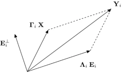
in the elimination of the term depending on the inputs and the nonlinearities in Eq. (15) using a geometrical projection. The two-dimensional interpretation of this equation depicted in Figure 3 shows that an orthogonal projection onto the orthogonal complement of Ei, denoted E⊥i , cancels the extended input term ΛiEi.
Matrix Γi can then be obtained by means of a truncated singular value decomposition of the result of the projection. The
truncation limits the singular value spectrum to genuine elements, hence removing spurious values and reducing the influence of noise and rounding errors on the identification. Moreover, the number of retained singular values yields the system order ns.
Yi
ΓiX
ΛiEi E⊥i
Figure 3: Geometrical interpretation of Eq. (15) in a two-dimensional space.
2.5 Estimation of the system matrices
From the knowledge of nsand cΓi, the next stage of the FNSI methodology is the computation of the four system matrices. As a
first step, A and C can be estimated by exploiting the shifted structure of Γi. This shift property writes
ΓiA = Γi (17)
where Γiand Γiare the matrix Γiwithout the last and first l rows. The state matrix A is thus found as the least-squares solution
of the overdetermined system of equations
b
A = cΓi †c
Γi (18)
where† is the pseudo-inverse, while the output matrix bCis extracted from cΓias its l first rows.
Matrices B and D are usually estimated in a second step as the solution of the least-squares optimisation problem b B, bD =arg min B,D Y(f) −[Cb ( zf Ins×ns− bA )−1 B + D ] E(f ) 2 . (19)
This approach may yield poor-quality results[1], because it basically requires the division between the output and extended input spectra. An alternative scheme was proposed in [3] and was found to be more robust than the solution of Eq. (19), in the sense that it performs reasonably well for most practical conditions. This scheme will therefore be used in the present study, but is not further detailed for conciseness.
2.6 Conversion from discrete-time state space to continuous-time physical space
The identified discrete-time model ( bA, bB, bC, bD)is first converted into the continuous-time domain[3], where the physical param-eters of the system, namely the underlying linear modal properties and the nonlinear coefficients ca,b, can next be estimated. To
achieve the transformation back to physical space, Eq. (2) is substituted into Eq. (1) in the frequency domain to yield
G−1(ω) Q(ω) + r ∑ a=1 sa ∑ b=1 ca,bHa,b(ω) = P(ω) (20)
where G(ω) is the FRF matrix of the underlying linear system, and where Q(ω), Ha,b(ω)and P(ω) are the Fourier transforms
of q(t), ha,b(t)and p(t), respectively. The concatenation of P(ω) and Ha,b(ω)further introduces the extended input spectrum E(ω), so as to obtain the linear relationship between Q(ω) and E(ω)
Q(ω) = G(ω)[ Inp×np −c
1,1Inp×np . . . −cr,srI
np×np ]E(ω) = Ge(ω) E(ω). (21)
Matrix Ge(ω), termed extended FRF matrix, encompasses the underlying linear FRF matrix of the system the nonlinear
coeffi-cients. Moreover, Ref. [15] proved that it is an invariant system property which can be retrieved, similarly to linear theory, from the combination of the continuous-time state-space matrices
Ge(ω) = cCc(j ω Ins×ns− cAc)−1Bcc+ cDc. (22)
As a result, the nonlinear coefficients identified from Ge
(ω)using Eqs. (21) and (22) are spectral quantities, i.e. they are complex-valued and frequency-dependent. This is an attractive property, because the importance of the frequency variations and imaginary parts of the coefficients is particularly convenient for assessing the quality of the identification results.
3 NONLINEAR NORMAL MODES
A brief overview of Nonlinear Normal Modes (NNMs) is given in this section for a better understanding of their evaluation and implementation in the system identification of the nonlinear beam. A detailed description with applications can be found in [5, 6].
3.1 Framework and definitions
There exist two main definitions of an NNM in the literature due to Rosenberg[16]and Shaw and Pierre[17]:
1. Targeting a straightforward nonlinear extension of the linear normal mode concept, Rosenberg defined an NNM motion as a vibration in unison of the system (i.e., a synchronous periodic oscillation).
2. To provide an extension of the NNM concept to damped systems, Shaw and Pierre defined an NNM as a two-dimensional invariant manifold in phase space. Such a manifold is invariant under the flow (i.e., orbits that start out in the manifold remain in it for all time), which generalizes the invariance property of linear normal modes to nonlinear systems.
At first glance, Rosenberg’s definition may appear restrictive in two cases. Firstly, it cannot be easily extended to nonconservative systems. However, the damped dynamics can often be interpreted based on the topological structure of the NNMs of the underlying conservative system[5]. Moreover, due to the lack of knowledge of damping mechanisms, engineering design in industry is often based on the conservative system, and this even for linear vibrating structures. Secondly, in the presence of internal resonances, the NNM motion is no longer synchronous, but it is still periodic. In the present study, an NNM motion is therefore defined as a (nonnecessarily synchronous) periodic motion of the undamped (Cv = 0) and unforced (p(t) = 0)
mechanical system in Eq. (1).
3.2 Frequency-Energy dependence
One typical dynamical feature of nonlinear systems is the frequency-energy dependence of their oscillations. As a result, the modal curves and frequencies of NNMs depend on the total energy in the system. In view of this dependence, the representation of NNMs in a frequency-energy plot (FEP) is particularly convenient. An NNM motion is represented by a point in the FEP, which is drawn at a frequency corresponding to the minimal period of the periodic motion and at an energy corresponding to the conserved total energy during the motion, which is the sum of the potential and kinetic energies. A branch is a family of NNM motions possessing the same qualitative features. A complete branch forms the so-called backbone of the mode, that in fact can be seen as the locus of forced resonances for varying energies.
3.3 Numerical computation
The extended definition of NNMs is particularly attractive when targeting their numerical computation. It enables the nonlinear modes to be effectively computed using algorithms for the continuation of periodic solutions, which are really quite sophisticated and advanced. Herein, the numerical method for the NNM computation relies on two main techniques, namely a shooting procedure and a method for the continuation of periodic solutions (i.e.,NNM motions). A detailed description of the numerical algorithm is given in [6]. The algorithm, as a combination of shooting and pseudo-arclength continuation methods, starts from the linear normal mode at low energy and proceeds with two steps: prediction-correction.
1. The predictor step is global and goes from one NNM motion at a specific energy level to another NNM motion at a somewhat different energy level.
2. The corrector step is local and refines the prediction to obtain the actual solution at a specific energy level.
3.4 Experimental evaluation
Vibration tests for linear structures belong to two main categories: Phase Resonance and Phase Separation methods. One approach belonging to the latter category was described in Section 2. On the other hand, phase resonance methods excite one mode at a time using multi-point sine excitation at the corresponding natural frequency. A careful selection of the shaker locations is required to induce single-mode behaviour. This process is also known as normal-mode tuning or force appropriation. In [7] the extension of Phase Resonance methods to nonlinear system is made using the NNM theory. According to the phase lag quadrature criterion a linear structure vibrates according to one of the normal modes if all degrees of freedom vibrate synchronously with a phase lag of 90 deg with respect to the harmonic excitation. This criterion can be generalised to monophase NNM motions of nonlinear structures, where the phase lag is defined with respect to each harmonic of the monophase signals. In other words, if the response (in terms of displacements or accelerations) across the structure is a monophase periodic motion in quadrature with the excitation, the structure vibrates according to a single NNM of the underlying conservative system. In practice a stepped sine excitation can be performed until the phase lag criterion is verified and a single NNM motion can be estimated for a specific energy. This is an appealing feature, at least for structures with relatively well-separated modes. This approach is considered in Section 6 to identify the experimental backbone of the first NNM motion of the beam with the softening-hardening nonlinear behaviour.
4 EXPERIMENTAL TESTS DESCRIPTION
The benchmark is a clamped-clamped beam composed by a main beam with a thin part at one end, as shown in Figure 4a. The
(a)
(b)
Figure 4: Experimental setup of the nonlinear beam.
Length (m) Width (m) Thickness (m)
Main beam 0.70 0.014 0.0140
Thin beam 0.04 0.014 0.0005
TABLE 1: Geometrical properties of the beam.
It is a monolithic structure made of 42CrMo4 steel and it includes also the clamping interface at the main-beam side. During the manufacturing process the thin beam suffered of an excessive bending stress, that caused the part to be curved with respect to the longitudinal direction of the main beam, as in Figure 4b where the clamping has been opened to show it. When the clamping enforces the thin beam to be straight, a local state of prestress is induced by the bending. This prestress was found to be responsible of softening nonlinearity for low excitation levels. Conversely, the high flexibility of the thin beam introduces a hardening geometrical nonlinearity when large deflections occur. The effect of gravity on the thin beam was avoided by adopting a vertical set-up with the exciter acting along the orthogonal direction (that is the out-of-plane direction of the thin beam). The structure is instrumented with 7 accelerometers which span the beam regularly. Besides, a shaker is used to apply random and stepped sine excitations, considering a sampling frequency of 1,600 Hz. Acceleration and force signals are recorded at the excitation point, located 0.3 m far from the clamped root, through an impedance head.
The signal acquisition is performed using the LMS SCADAS mobile and among all the LMS Test.LAB Structures Acquisition programs, the MIMO FRF testing and MIMO Stepped Sine testing are used for the subspace and the nonlinear normal modes-based system identification, respectively. Specifically the former implements also arbitrary user-defined signals as excitations and this allows the definition of a periodic random signal with a user-controlled amplitude spectrum for the optimal application of FNSI. In this study, a flat spectrum is selected in the [5− 600] Hz band, and 80 periods of 214samples were considered. In order to let the lightly damped system reach the stationary condition 40 periods are first rejected and then the responses are averaged over the 40 remaining periods for mitigating noise. Six different levels of excitation are considered from 0.83 N to 25.04 N in terms of root mean square (rms) of the random signal.
Once a finite element model of the beam with the nonlinearity can be implemented from the FNSI results, the aim would be the evaluation of a forced response at a specific excitation level to be compared to the experimental responses when a stepped sine signal is fed the shaker. Since a weak coupling between the shaker and the beam occurs, the force measured at the interface evidences a decrease of the amplitude when approaching resonance. This effect cannot be completely removed and prevent to achieve exactly the same condition of the numerical simulations, since any attempt to control in a close-loop test the excitation level to be stable would result in an continuous jump from low to high (and vice-versa) energy branches of the nonlinear system. Nevertheless, the experimental harmonic forces and accelerations are measured in a stationary condition (reached after about 10 periods) for about 10 periods and the corresponding amplitude and phase values can be estimated for each known frequency. This results in the assessment of the experimental NNMs that can be directly compared with the numerical evaluations coming from the implementation of the finite element model in an already developed continuation toolbox[6]capable to handle user-defined nonlinear forces.
5 FREQUENCY NONLINEAR SUBSYSTEM IDENTIFICATION OF THE BEAM
The low level random test was repeated five times to check that the boundary conditions were not changing during the tests. These several non consecutive tests can be used to evaluate the uncertainty related to the modal parameters estimated for the characterization of the system linear behaviour. The first three bending modes of the beam belong to the analysed bandwidth and are summarised in Table 2 together with the associated uncertainties.
Mode natural frequency (Hz) damping ratio (%)
1 31.63± 0.09 0.458± 0.051
2 147.82± 0.03 0.027± 0.002
3 407.11± 0.04 0.119± 0.014
TABLE 2: Experimental linear modes of the beam as assessed from random tests at low excitation level (0.83 Nrms).
When the excitation level is increased the softening-hardening nonlinearity affects the peak of the frequency response functions at the resonances. Specifically, for excitation levels up to about 12 Nrms the first mode moves towards lower frequencies
(symptom of a softening behaviour), but for higher energy regimes this resonance shifts to the right (symptom of a hardening behaviour). Figure 5 shows a close up around the first resonance of the frequency response functions at the tip of the main beam for three excitation levels: the lowest level (0.83 Nrms in red), a regime in which the softening behaviour prevails (6.00 Nrms in blue) and the highest level (25.04 Nrms in gray). It can be also noted that the FRFs become more ”noisy” when the excitation increases as a further indicator of nonlinear mechanisms acting in the system.
15 20 25 30 35 40 45 50 −100 −95 −90 −85 −80 −75 −70 −65 −60 −55 −50 Frequency (Hz)
FRF at main beam tip (dB)
25.04 N rms 6.00 Nrms 0.83 N
rms
Figure 5: Frequency response functions at the tip of the main beam for excitation levels equal to 0.83 Nrms (red solid line), 6.00 Nrms (blue solid line) and 25.04 Nrms (gray solid line).
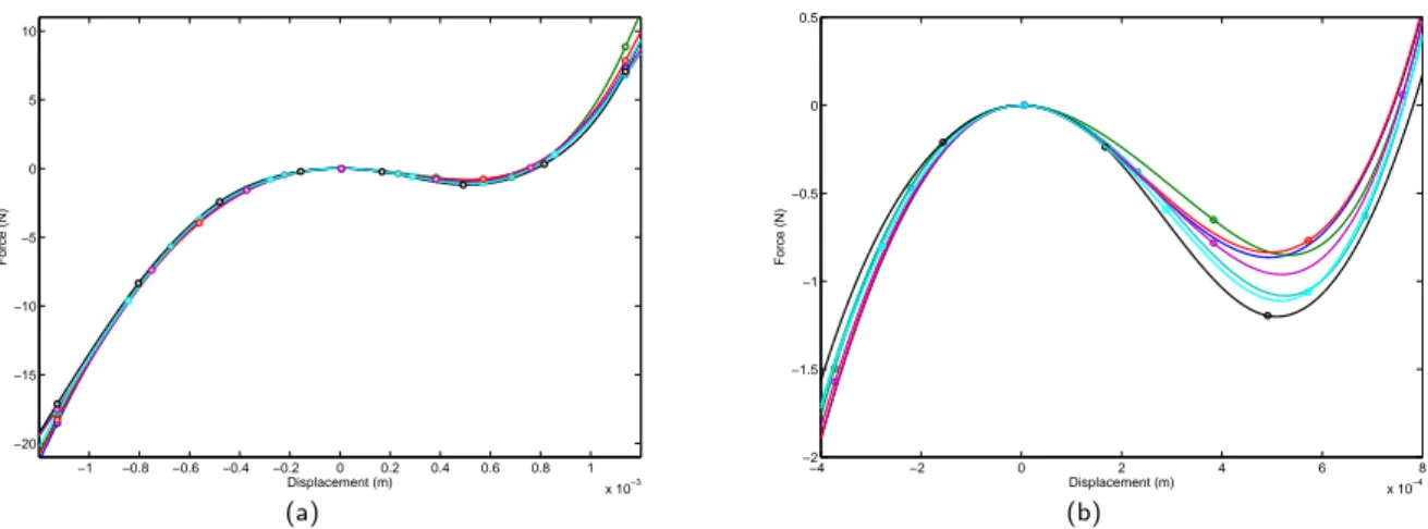
The FNSI method is applied to the high-energy test case (25.04 Nrms) in order to estimate the extended FRF matrix, so then the underlying linear FRF matrix of the system and the coefficients of the nonlinear input force acting at the main beam tip. The latter is considered to be completely unknown and generic cubic splines are implemented to fit its behaviour. Figure 6 shows the estimated functions, when the frequency samples are processed within the bandwidth [5-600] Hz and several intervals defying the splines are considered, as indicated by the points on each curve. Specifically, in the present study, the range of the analysis, that is±1.1 mm, is divided in a number of intervals ranging from two up to eight. All the functions interpolating the restoring force well represent the softening-hardening behaviour within the range of the analysis. The force, in fact, increases with the displacement following the hardening characterization of the nonlinearity except for a small range of positive displacements in which the softening is prevailing, as highlighted in Figure 6b. It is worth noting that the more the splines used to fit the data the more pronounced is the dip representing the softening behaviour, whereas the hardening characterization is almost not affected.
Besides, the FNSI method is exploited to reconstruct the FRFs of the underlying linear system and therefore to estimate the modal parameters from the high-energy test. In this case, the natural frequency closely matches the low-level property with a relative error of−0.97%, −0.20% and −0.04% on the three modes, respectively. The damping ratio is also satisfactorily estimated with larger relative errors equal to 6.62%, 25.09% and 20.50% for the three modes, respectively. These errors on the damping ratios are not necessarily to be attributed to nonlinear damping, but can also translate modelling errors. Figure 7 compares the driving-point FRFs around the first resonance as assessed by using the H1 estimator on the experimental data in case of
−1 −0.8 −0.6 −0.4 −0.2 0 0.2 0.4 0.6 0.8 1 x 10⁻³ −20 −15 −10 −5 0 5 10 Displacement (m) Force (N) (a) −4 −2 0 2 4 6 8 x 10⁻⁴ −2 −1.5 −1 −0.5 0 0.5 Displacement (m) Force (N) (b)
Figure 6: Restoring force acting at the main beam tip as estimated by FNSI using different splines.
the lowest and the highest level of excitation (0.83 Nrms in red and 25.04 Nrms in gray, respectively) with the reconstruction coming from the FNSI method (25.04 Nrms in black). It can be noted that the estimate of the underlying linear FRF as from FNSI matches the experimental FRF at the lowest level of excitation. The frequency-shift of the resonance peak due to the nonlinearity is recovered, although the relative error of−0.97% on the first natural frequency can be highlighted.
15 20 25 30 35 40 45 50 −30 −20 −10 0 10 20 30 Frequency (Hz) Driving−point FRF (dB) 25.04 N rms 0.83 N rms FNSI 25.04 Nrms
Figure 7: Driving-point frequency response function for excitation level equal to 25.04 Nrms as estimated using FNSI (black solid line) compared with the experimental FRF at the same and at the lowest level of excitation (gray and red solid line, respectively).
6 NNM-BASED IDENTIFICATION OF THE BEAM
Starting from the parameters estimated by FNSI a finite element model of the two beams has been implemented, such that the linear modal parameters were the same of the real structure, assuming the damping matrix to be proportional to the mass and stiffness matrices. The nonlinear force acting at the tip of the main beam has been added to the system as identified by FNSI using cubic splines. In the following the analyses are focused on the first mode which involves the largest displacement of the main beam tip, that is where the geometrical nonlinearity is acting, and hence the strongest effects are addressed.
24 26 28 30 32 34 36 38 40 42 44 10−2 10−1 100 101 Frequency (Hz) Acceleration (g)
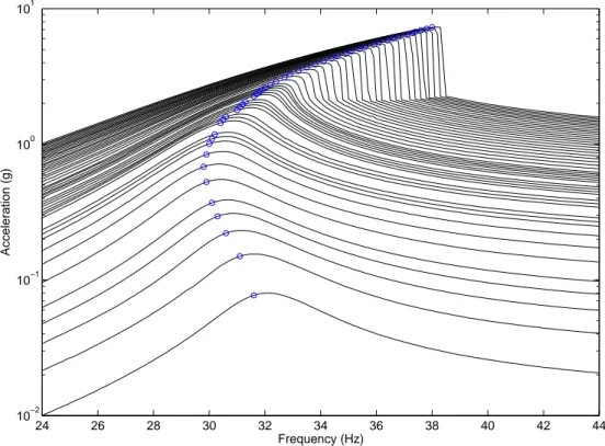
Figure 8: Experimental response functions at the main beam tip to several stepped sine excitations at different energies with highlighted the points where the quadrature condition is fulfilled.
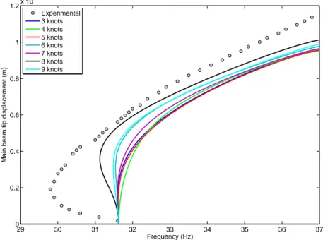
The experimental harmonic forces and accelerations are measured in stationary conditions for varying frequency at different excitation energies. When a 90 deg of phase shift is detected between the force and the acceleration, the resonance is occurring since the quadrature condition is fulfilled. At this point an estimate of the nonlinear normal mode can be experimentally achieved and compared with the analogous coming from the numerical evaluation of the backbone from the nonlinear normal mode continuation toolbox. Figure 8 shows the experimental harmonic response of the main beam tip for harmonic excitation ranging from 0.01 N to 0.88 N. Both up and down sweep directions were tested, but only the former is here represented for the sake of brevity. It can be noted that at first the curves tend to bend to the left and then to the right, as expected by the softening-hardening behaviour already identified in the previous section. Moreover, for high excitations the so-called jump phenomenon appears, that is when suddenly the response amplitude strongly decreases (or increases) for a small increase (or decrease) of the excitation frequency in case of the hardening behaviour. Since the presence of structural damping the resonances are not located at the peak of the responses and these jumps happen after the achievement of the quadrature condition, so at higher frequencies. Figure 9 compares the experimental resonances with the numerical backbone when different restoring force functions acting at the main beam tip are considered as estimated by FNSI using different splines (see Figure 6). Herein the splines are charac-terised by the number of knots used to defined them. High sensitivity of the numerical backbone to the nonlinear force can be noted. The resonances depend on the total energy in the system and the nonlinear restoring force plays an important role on their evaluation. For displacements higher than 0.8 mm the hardening behaviour is mostly affecting the nonlinear dynamics and
the numerical backbones tend to a similar trend, as for the restoring force splines in Figure 6. Conversely, if the softening be-haviour is prevailing, different estimates of the restoring force result in remarkable variations of the NNM evaluation. Specifically the NNM frequency reaches smaller values if the corresponding restoring force has a more pronounced dip. Although none of the numerical results matches the values along the experimental backbone, the capability of catching analogous dynamics is a remarkable features of the model; nonlinear model updating can be performed to let the two estimates match.
29 30 31 32 33 34 35 36 37 0 0.2 0.4 0.6 0.8 1 1.2x 10 −3 Frequency (Hz)
Main beam tip displacement (m)
Experimental 3 knots 4 knots 5 knots 6 knots 7 knots 8 knots 9 knots
Figure 9: Comparison between the experimental (circles) with the numerical first NNM backbone for different splines interpolating the nonlinear restoring force.
As a final remark, the splines are estimated by enforcing them to pass through the origin with a zero slope (for null displacement the nonlinear force and its first derivative are zero); when an odd number of knots is therefore considered, one of the knots is close to the origin and an almost redundant condition is used to solve the system that defines the spline coefficients. This results in more accurate splines in case of even number of knots. In future different distributions of these knots within the range of interest is going to be analysed also to improve the assessment of the softening behaviour induced by the prestess.
7 CONCLUDING REMARKS
In this paper the system identification of a nonlinear beam was carried out based on experimental tests and numerical sim-ulations. The focus was put onto the first mode of vibration involving both softening and hardening effects. With this aim, a frequency-domain nonlinear generalisation of subspace methods, referred to as the FNSI method, was exploited. The corre-sponding linear and nonlinear parameters were estimated allowing the formulation of an accurate finite element model. Taking advantage of numerical continuation techniques the backbone of the first nonlinear normal mode was identified and compared to the experimental achievements with good results, although better accuracy in the definition of the nonlinearity could be obtained as means of nonlinear updating or using a fully nonlinear finite element model of the beam. Two different kinds of excitation were considered for the system identification and the complex softening-hardening behaviour was assessed by both of them. However, additional experimental investigations can be performed to further understand the dynamics of the structure so as to correlate also other features of nonlinear systems, such as the modal interaction.
ACKNOWLEDGEMENTS
The authors Chiara Grappasonni and Gaetan Kerschen would like to ackonwledge the financial support of the European Union (ERC Starting Grant NoVib 307265).
The authors also want to thank LMS A Siemens Business for providing access to the LMS Test.Lab software.
The author Jean-Philippe No ¨el is a Research Fellow (FRIA fellowship) of the Fonds de la Recherche Scientifique – FNRS which is gratefully acknowledged.
REFERENCES
[1] Van Overschee, P. and De Moor, B., Subspace Identification for Linear Systems: Theory - Implementation - Applications, Kluwer Academic Publishers, Boston/London/Dordrecht, 1st edn., 1996.
[2] McKelvey, T., Akcay, H. and Ljung, L., Subspace-based multivariable system identification from frequency response data, IEEE Transactions on Automatic Control, Vol. 41, pp. 960–979, 1996.
[3] No ¨el, J. P. and Kerschen, G., Frequency-domain subspace identification for nonlinear mechanical systems, Mechanical Systems and Signal Processing, Vol. 40, pp. 701–717, 2013.
[4] Kerschen, G., Worden, K., Vakakis, A. and Golinval, J.-C., Past, present and future of nonlinear system identification in
structural dynamics, Mechanical Systems and Signal Processing, Vol. 20, pp. 505–592, 2006.
[5] Kerschen, G., Peeters, M., Golinval, J.-C. and Vakakis, A., Nonlinear normal modes, PartI: A useful framework for the
structural dynamicist, Mechanical Systems and Signal Processing, Vol. 23, pp. 170–194, 2009.
[6] Peeters, M., Vigui ´e, R., S ´erandour, G., Kerschen, G. and Golinval, J.-C., Nonlinear normal modes, Part II: Toward a
practical computation using numerical continuation techniques, Mechanical Systems and Signal Processing, Vol. 23, No. 1,
pp. 195 – 216, 2009.
[7] Peeters, M., Kerschen, G. and Golinval, J., Dynamic testing of nonlinear vibrating structures using nonlinear normal
modes, Journal of Sound and Vibration, Vol. 330, No. 3, pp. 486 – 509, 2011.
[8] Thouverez, F., Presentation of the ECL benchmark, Mechanical Systems and Signal Processing, Vol. 17, No. 1, pp. 195 – 202, 2003.
[9] Adams, D. E. and Allemang, R. J., A frequency domain method for estimating the parameters of a non-linear structural
dynamic model through feedback, Mechanical Systems and Signal Processing, Vol. 14, No. 4, pp. 637–656, 2000.
[10] Pintelon, R. and Schoukens, J., System Identification: A Frequency Domain Approach, IEEE Press, New York, 1st edn., 2001.
[11] Schetzen, M., The Volterra and Wiener Theories of Nonlinear Systems, Wiley, New York, 1st edn., 1980.
[12] Schoukens, J., Pintelon, R., Rolain, Y. and Dobrowiecki, T., Frequency response function measurements in the presence
of nonlinear distortions, Automatica, Vol. 37, pp. 939–946, 2001.
[13] Van Overschee, P. and De Moor, B., Continuous-time frequency domain subspace system identification, Signal Process-ing, Vol. 52, pp. 179–194, 1996.
[14] Yang, Z. and Sanada, S., Frequency domain subspace identification with the aid of the w-operator, Electrical Engineering in Japan, Vol. 132, No. 1, pp. 46–56, 2000.
[15] Marchesiello, S. and Garibaldi, L., A time domain approach for identifying nonlinear vibrating structures by subspace
methods, Mechanical Systems and Signal Processing, Vol. 22, pp. 81–101, 2008.
[16] Rosenberg, R., Normal modes of nonlinear dual-mode systems, Journal of Applied Mechanics, Vol. 27, No. 2, pp. 263–268, 1960.
[17] Shaw, S. and Pierre, C., Non linear normal modes and invariant manifolds, Journal of Sound and Vibration, Vol. 150, No. 1, pp. 170–173, 1991.
![Figure 2: Feedback interpretation of nonlinear structural dynamics [9] .](https://thumb-eu.123doks.com/thumbv2/123doknet/6017150.150248/4.892.204.714.126.305/figure-feedback-interpretation-nonlinear-structural-dynamics.webp)