Dealing with the Inventory Risk
Olivier Guéant, Charles-Albert Lehalle, Joaquin Fernandez Tapia
Les Cahiers de la Chaire / N°43
Dealing with the Inventory Risk
Olivier Gu´
eant
∗, Charles-Albert Lehalle
∗∗, Joaquin Fernandez Tapia
∗∗∗2010
Abstract
Market makers have to continuously set bid and ask quotes for the stocks they have under consideration. Hence they face a complex optimization problem in which their return, based on the bid-ask spread they quote and the frequency they indeed provide liquidity, is chal-lenged by the price risk they bear due to their inventory. In this paper, we provide optimal bid and ask quotes and closed-form approximations are derived using spectral arguments.
Introduction
The optimization of the intra-day trading process on electronic markets was born with the need to split large trades to make the balance between trading too fast (and possibly degrade the obtained price via “market impact”) and trading too slow (and suffer from a too long exposure to “market risk”). This “trade scheduling” viewpoint has been mainly formalized in the late nineties by Bertsimas and Lo [8] and Almgren and Chriss [2]. More sophisticated approaches involving the use of stochastic and impulse control have been proposed since then (see for instance [9]). Another branch of proposals goes in the direction of modeling the effect of the “aggressive” (i.e. liquidity consuming) orders at the finest level, for instance via a martingale model of the behavior market depth and of its resilience (see [1]).
From a quantitative viewpoint, market microstructure is a sequence of auction games be-tween market participants. It implements the balance bebe-tween supply and demand, forming an equilibrium traded price to be used as reference for valuation of the listed assets. The rule of each auction game (fixing auction, continuous auction, etc), are fixed by the firm operating each trading venue. Nevertheless, most of all trading mechanisms on electronic markets rely on market participants sending orders to a “queuing system” where their open interests are consolidated as “liquidity provision” or form transactions [3]. The efficiency of such a process relies on an adequate timing between buyers and sellers, to avoid too many non-informative oscillations of the transaction price (for more details and modeling, see for example [19]).
To take profit of these oscillations, it is possible to provide liquidity to an impatient buyer (respectively seller) and maintain an inventory until the arrival of the next impatient seller
The authors wish to acknowledge the helpful conversations with Pierre-Louis Lions (Coll`ege de France),
Jean-Michel Lasry (Universit´e Paris-Dauphine), Yves Achdou (Universit´e Paris-Diderot), Thierry Foucault (HEC),
Albert Menkveld (VU University Amsterdam), Vincent Millot (Universit´e Paris-Diderot), Antoine Lemenant
(Uni-versit´e Paris-Diderot) and Vincent Fardeau (London School of Economics).
∗UFR de Math´ematiques, Laboratoire Jacques-Louis Lions, Universit´e Paris-Diderot. 175, rue du Chevaleret,
75013 Paris, France. [email protected]
∗∗Head of Quantitative Research. Cr´edit Agricole Cheuvreux. 9, Quai du Pr´esident Paul Doumer, 92400
Courbevoie, France. [email protected]
(respectively buyer). Market participants focused on this kind of liquidity-providing activity are called “market makers”. On one hand they are buying at the bid price and selling at the ask price they chose, taking profit of this “bid-ask spread”. On the other hand, their inventory is exposed to price fluctuations mainly driven by the volatility of the market (see [4, 7, 11, 13, 16, 23]).
The usual “market making problem” comes from the optimality of the quotes (i.e. the bid and ask prices) that such agents provide to other market participants with respect to the constraints on their inventory and their utility function as a proxy to their risk (see [10, 15, 17, 20, 22, 25]).
The recent evolution of market microstructure and the financial crisis reshaped the nature of the interactions of the market participants during electronic auctions, one consequence being the emergence of “high-frequency market makers” who are said to be part of 70% of the electronic trades and have a massively passive (i.e. liquidity providing) behavior. A typical balance between passive and aggressive orders for such market participants is around 80% of passive interactions (see [21]).
Avellaneda and Sto¨ıkov proposed in [5] an innovative framework for “market making in an order book” and studied it using different approximations. In such an approach, the “fair
price” St is modeled via a Brownian motion with volatility σ, and the arrival of a buy or
sell liquidity-consuming order at a distance δ of St follows a Poisson process with intensity
A exp(−k δ). Our paper extends their proposal and provides results in two main directions:
• An explicit solution to the Hamilton-Jacobi-Bellman equation coming from the optimal
market making problem thanks to a non trivial change of variables and the resulting expressions for the optimal quotes:
Main Result 1 (Theorems 1-2). The optimal quotes can be expressed as:
sb∗(t, q, s) = s− ( −1 kln ( vq+1(t) vq(t) ) +1 γ ln ( 1 +γ k )) sa∗(t, q, s) = s + ( 1 kln ( vq(t) vq−1(t) ) + 1 γ ln ( 1 +γ k ))
where γ is the risk aversion of the agent and where v is a family of strictly positive
functions (vq)q∈Z solution of the linear system of ODEs (S) that follows:
∀q ∈ Z, ˙vq(t) = αq2vq(t)− η (vq−1(t) + vq+1(t))
with vq(T ) = 1, and α = k2γσ2 and η = A(1 + γk)−(1+
k γ).
It means that to find an exact solution to the generic high-frequency market making problem, it is enough to solve on the fly the companion ODEs in vq(t) provided by our
change of variables, and to plug the result in the upper equalities to obtain the optimal quotes with respect to a given inventory and market state.
• Asymptotics of the solution that are numerically attained fast enough in most realistic
cases:
Main Result 2 (Theorem 3 (asymptotics) and the associated approximation
equa-tions). lim T→∞s− s b∗(0, q, s) = δb∗ ∞(q) ≃ γ1ln ( 1 +γ k ) +2q + 1 2 √ σ2γ 2kA ( 1 +γ k )1+kγ lim sa∗(0, q, s)− s = δ∞a∗(q) ≃ 1ln ( 1 +γ ) −2q− 1 √ σ2γ ( 1 +γ )1+kγ
These results open doors to new directions of research involving the modeling and con-trol of passive interactions with electronic order books. If some attempts have been made that did not rely on stochastic control but on forward optimization (see for instance [24] for a stochastic algorithmic approach for optimal split of passive orders across competing electronic order books), they should be complemented by backward ones.
This paper goes from the description of the model choices that had to be made (section 1), through the main change of variables (section 2), exposes the asymptotics of the obtained dynamics (section 3), its comparative statics (section 4), extends the framework to trends in prices and constraints on the inventory (section 5), finally discusses the model choices that had to be made (section 6) and ends with an application to real data (section 7). Adaptations of our results are already in use at Cr´edit Agricole Cheuvreux to optimize the brokerage trading flow.
In our framework, we follow Avellaneda and Sto¨ıkov in using a Poisson process model pegged on a “fair price” diffusion (see section 1). As it is discussed in section 6, it is an arguable choice since it does not capture “resistances” that can be built by huge passive (i.e. liquidity-providing) orders preventing the market price to cross their prices. Our results cannot be used as such for large orders, but are perfectly suited for high-frequency market making as it is currently implemented in the market, using orders of small size (close to the average trade size, see [21]).
Moreover, to our knowledge, no quantitative model of “implicit market impact” of such small passive orders has never been proposed in the literature, despite very promising studies linking updates of quantities in the order books to price changes (see [12]). Its combination with recent applications of more general point processes to capture the process of arrival of orders (like Hawkes models, see [6]) should give birth to such implicit market impact models, specifying dependencies between the trend, the volatility and possible jumps in the “fair price” semi-martingale process with the parameters of the multi-dimensional point process of the market maker fill rate. At this stage, the explicit injection of such path-dependent approach (once they will be proposed in the literature) into our equations are too complex to be handled, but numerical explorations around our explicit formulas will be feasible. The outcomes of applications of our results to real data (section 7) show that they are realistic enough so that no more that small perturbations should be needed.
1
Setup of the model
1.1
Prices and Orders
We consider a small high-frequency market maker operating on a single stock1. For the sake of simplicity and since we will basically only consider short horizon problems we suppose that the mid-price of the stock moves as a brownian motion:
dSt= σdWt
The market maker under consideration will continuously propose bid and ask quotes denoted respectively Sbt and Staand will hence buy and sell stocks according to the rate of arrival of aggressive orders at the quoted prices.
His inventory q, that is the (signed) quantity of stocks he holds, is given by qt= Ntb− Nta
where Nb and Na are the jump processes giving the number of stocks the market maker respectively bought and sold. These jump processes are supposed to be Poisson processes and to simplify the exposition (although this may be important, see the discussion part)
1We suppose that this high-frequency market maker does not “make” the price in the sense that he has no
market power. In other words, we assume that his size is small enough to consider price dynamics exogenous. Small high-frequency proprietary trader operating on both sides would be another way to describe our agent.
we consider that jumps are of size 1. Arrival rates obviously depend on the prices Stb and
Sa
t quoted by the market maker and we assume, in accordance with most datasets, that
intensities λb and λa associated to Nb and Na are of the following form2:
λb(sb, s) = A exp(−k(s − sb)) λa(sa, s) = A exp(−k(sa− s))
This means that the closer to the mid-price an order is quoted, the faster it will be executed. As a consequence of his trades, the market maker has an amount of cash whose dynamics is given by:
dXt= StadNta− StbdNtb
1.2
The optimization problem
As we said above, the market maker has a time horizon T and his goal is to optimize the expected utility of his P&L at time T . In line with [5], we will focus on CARA utility functions and we suppose that the market maker optimizes:
sup
Sa,Sb
E [− exp (−γ(XT + qTST))]
where γ is the absolute risk aversion characterizing the market maker, where XT is the
amount of cash at time T and where qTST is the mid-price evaluation of the (signed)
re-maining quantity of stocks in the inventory at time T (liquidation at mid-price3).
2
Resolution
2.1
Hamilton-Jacobi-Bellman equation
The optimization problem set up in the preceding section can be solved using classical Bellman tools. To this purpose, we introduce a Bellman function u defined as:
u(t, x, q, s) = sup
Sa,Sb
E [− exp (−γ(XT + qTST))| Xt= x, St= s, qt= q]
The Hamilton-Jacobi-Bellman equation associated to the optimization problem is then given by the following proposition:
Proposition 1 (HJB). The Hamilton-Jacobi-Bellman equation for u is:
(HJB) 0 = ∂tu(t, x, q, s) + 1 2σ 2∂2 ssu(t, x, q, s) + sup sb λb(sb, s) [ u(t, x− sb, q + 1, s)− u(t, x, q, s) ] + sup sa λ a(sa, s) [u(t, x + sa, q− 1, s) − u(t, x, q, s)]
with the final condition:
u(T, x, q, s) =− exp (−γ(x + qs))
This equation is not a simple 4-variable PDE. Rather, because the inventory is discrete, it is an infinite system of 3-variable PDEs. To solve it, we will use a change of variables that is different from the one used in [5] and transforms the system of PDEs in a system of linear ODEs.
2Although this form is in accordance with real data, some authors used a linear form for the intensity functions
2.2
Reduction to a system of linear ODEs
In [5], the authors proposed a change of variables to factor out wealth. Here we go further and propose a rather non-intuitive change of variables that allows to write the problem in a linear way.
Proposition 2 (A system of linear ODEs). Let’s consider a family of strictly positive
func-tions (vq)q∈Z solution of the linear system of ODEs (S) that follows:
∀q ∈ Z, ˙vq(t) = αq2vq(t)− η (vq−1(t) + vq+1(t))
with vq(T ) = 1, where α = k2γσ2 and η = A(1 +γk)−(1+
k γ).
Then u(t, x, q, s) =− exp(−γ(x + qs))vq(t)−
γ
k is solution of (HJB).
Theorem 1 (Well-posedness of the system (S)). There exists a unique solution of (S) in
C∞([0, T ), ℓ2(Z)) and this solution consists in strictly positive functions.
2.3
Optimal quotes characterization
Theorem 2 (Optimal quotes and bid-ask spread). Let’s consider the solution v of the system
(S) as in Theorem 1. Then optimal quotes can be expressed as:
sb∗(t, q, s) = s− ( −1 kln ( vq+1(t) vq(t) ) + 1 γ ln ( 1 +γ k )) sa∗(t, q, s) = s + ( 1 kln ( vq(t) vq−1(t) ) +1 γ ln ( 1 +γ k ))
Moreover, the bid-ask spread quoted by the market maker, that is ψ∗ = sa∗(t, q, s)−sb∗(t, q, s),
is given by: ψ∗(t, q) =−1 kln ( vq+1(t)vq−1(t) vq(t)2 ) + 2 γ ln ( 1 +γ k )
We see that the difference between each quoted price and the mid-price has two compo-nents. If we consider the case of the bid quote – the same analysis would be true in the case of the ask quote –, we need to separate the term −k1ln
(
vq+1(t)
vq(t)
)
from the term 1γln(1 +γk). If σ = 0, then vq(t) = exp(2η(T − t)) defines a solution of the system (S). Hence, the
relations s− sb∗ = sa∗ − s = 1γln(1 +γk) define the optimal quotes in the “no-volatility” benchmark case4. Consequently, in the expression that defines the optimal quotes, the sec-ond term correspsec-onds to the “no-volatility” benchmark while the first one takes account of the influence of volatility.
3
Examples and asymptotics
To motivate the asymptotic approximation we provide, and before discussing the way to solve the problem numerically, let us present some graphs to understand the behavior in time and inventory of both the optimal quotes and the bid-ask spread.
4Smaller quotes would lead to trade more often with less revenue per trade in a way that is not in favor of the
market maker. Symmetrically, larger quotes would lead to more revenue per trade but less trades and the welfare of the market maker would also be reduced.
3.1
Numerical examples
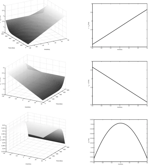
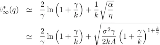
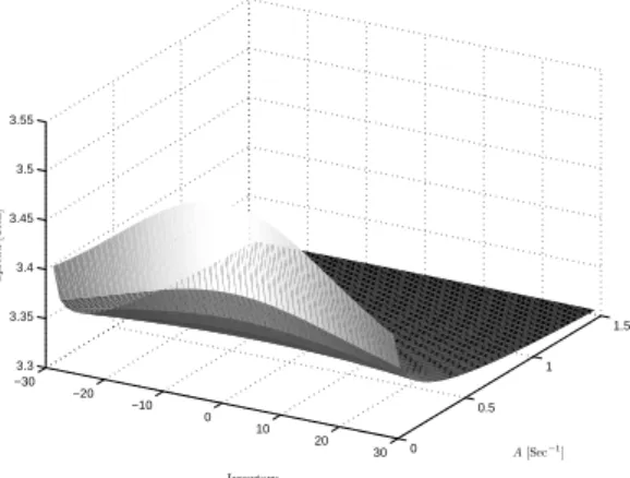
−30 −20 −10 0 10 20 30 0 100 200 300 400 500 600 0.5 1 1.5 2 2.5 3 Inventory Time [Sec] s − s b [Tick] −30 −20 −10 0 10 20 30 0.5 1 1.5 2 2.5 3 Inventory s − s b [Tick] −30 −20 −10 0 10 20 30 0 100 200 300 400 500 600 0.5 1 1.5 2 2.5 3 Time [Sec] Inventory sa − s [Tick] −30 −20 −10 0 10 20 30 0.5 1 1.5 2 2.5 3 Inventory sa − s [Tick] −30 −20 −10 0 10 20 30 0 100 200 300 400 500 600 3.275 3.28 3.285 3.29 3.295 3.3 3.305 3.31 3.315 3.32 Time [Sec] Inventory ψ [Tick] −30 −20 −10 0 10 20 30 3.3114 3.3116 3.3118 3.312 3.3122 3.3124 3.3126 3.3128 3.313 3.3132 Inventory ψ [ Tick ]Figure 1: Left: Behavior of the optimal quotes and bid-ask spread with time and inventory. Right: Behavior of the optimal quotes and bid-ask spread with inventory, at time t = 0. σ = 0.3 Tick· s−1/2, A = 0.9 s−1, k = 0.3 Tick−1, γ = 0.01 Tick−1, T = 600 s.
3.2
Asymptotics
In [5], the authors propose a heuristic approximation for the bid-ask spread. Namely they propose to approximate ψ∗(t, q) by γσ2(T− t) +2γln(1 +γk). However, as suggested by the graphs exhibited above, the predominant feature is that both the bid-ask spread and the distance between the quotes and the mid-price are rather constant, except near the time horizon T (and in numerical examples, a few minutes are enough to be near the asymptotic values), and certainly not linearly decreasing with time.
In fact, we can prove the existence of an asymptotic behavior and provide semi-explicit expressions for the asymptotic values of the bid-ask spread and the quotes:
Theorem 3 (Asymptotic quotes and bid-ask spread).
∀q ∈ Z, ∃δb∗ ∞(q), δa∞∗(q), ψ∗∞(q)∈ R lim T→∞s− s b∗(0, q, s) = δb∗ ∞(q) lim T→∞s a∗(0, q, s)− s = δa∗ ∞(q) lim T→∞ψ ∗(0, q) = ψ∗ ∞(q) Moreover, δb∞∗(q) = 1 γ ln ( 1 +γ k ) − 1 kln ( fq+10 f0 q ) δ∞a∗(q) = 1 γ ln ( 1 +γ k ) +1 kln ( fq0 f0 q−1 ) and ψ∗∞(q) =−1 kln ( f0 q+1fq0−1 f0 q2 ) +2 γ ln ( 1 +γ k )
where f0 ∈ ℓ2(Z) is characterized by:
f0∈ argmin ∥f∥ℓ2(Z)=1 ∑ q∈Z αq2fq2+ η∑ q∈Z (fq+1− fq)2
As we have seen in the above numerical examples, only these asymptotic values seem to be relevant in practice. Consequently, we provide an approximation for f0 that happens to fit the actual figures. This approximation is based on the continuous counterpart of f0, namely ˜f0 ∈ L2(R), a function that verifies:
˜ f0 ∈ argmin ∥ ˜f∥L2(R)=1 ∫ ∞ −∞ ( αx2f (x)˜ 2+ η ˜f′(x)2 ) dx
It can be proved5 that such a function ˜f0 must be proportional to the probability distri-bution function of a normal variable with mean 0 and variance
√ η α. Hence, we expect f 0 q to behave as exp ( −1 2 √ α ηq 2).
This heuristic viewpoint induces an approximation for the optimal quotes and bid-ask spread if we replace fq0 by exp
( −1 2 √ α ηq 2): δb∞∗(q) ≃ 1 γ ln ( 1 +γ k ) + 1 2k √ α η(2q + 1) ≃ 1 γ ln ( 1 +γ k ) +2q + 1 2 √ σ2γ 2kA ( 1 +γ k )1+kγ δ∞a∗(q) ≃ 1 γ ln ( 1 +γ k ) − 1 2k √ α η(2q− 1) ≃ 1 γ ln ( 1 +γ k ) −2q− 1 2 √ σ2γ 2kA ( 1 +γ k )1+k γ
5To prove this we need to proceed as in the proof of Theorems 1 and 3. In a few words, we introduce the positive,
compact and self-adjoint operator Lc defined for f ∈ L2(R) as the unique weak solution v of αx2v− ηv′′ = f
with∫−∞∞ (αx2v(x)2+ ηv′(x)2)dx < +∞. L
c can be diagonalized and largest eigenvalue of Lc can be shown to
be associated to the eigenvector f (x) = exp ( −1 2 √ α ηx 2).
ψ∗∞(q) ≃ 2 γ ln ( 1 +γ k ) +1 k √ α η ≃ 2 γ ln ( 1 +γ k ) + √ σ2γ 2kA ( 1 +γ k )1+kγ
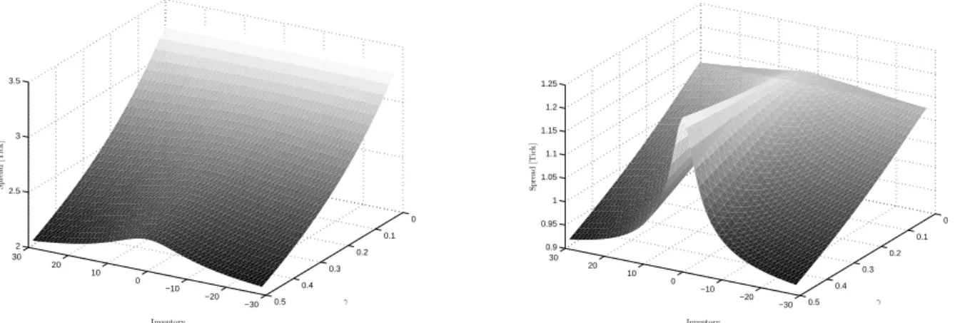
We exhibit below the values of the optimal quotes and the bid-ask spread, both with their associated approximations. Empirically, these approximations for the quotes are satisfactory in most cases and are always good for small values of the inventory q. The apparent difficulty to approximate the bid-ask spread comes from the chosen scale (the bid-ask spread being almost uniform across values of the inventory).
−300 −20 −10 0 10 20 30 0.5 1 1.5 2 2.5 3 3.5 Inventory s − s b [Tick] −30 −20 −10 0 10 20 30 −6 −4 −2 0 2 4 6 8 10 Inventory s − s b [Tick] −300 −20 −10 0 10 20 30 0.5 1 1.5 2 2.5 3 3.5 Inventory sa − s [Tick] −30 −20 −10 0 10 20 30 −6 −4 −2 0 2 4 6 8 10 Inventory sa − s [Tick] −30 −20 −10 0 10 20 30 3.321 3.3215 3.322 3.3225 3.323 3.3235 3.324 3.3245 Inventory ψ [Tick] −30 −20 −10 0 10 20 30 3.36 3.38 3.4 3.42 3.44 3.46 3.48 3.5 3.52 3.54 3.56 Inventory ψ [Tick]
Figure 2: Asymptotic behavior of optimal quotes and the bid-ask spread (bold line). Approxima-tion (dotted line). Left: σ = 0.4 Tick· s−1/2, A = 0.9 s−1, k = 0.3 Tick−1, γ = 0.01 Tick−1,
T = 600 s. Right: σ = 1.0 Tick· s−1/2, A = 0.2 s−1, k = 0.3 Tick−1, γ = 0.01 Tick−1,
4
Comparative statics
Before starting with the comparative statics, we rewrite the approximations done in the previous section to be able to have some intuition about the behavior of the optimal quotes and bid-ask spread with respect to the parameters:
δ∞b∗(q)≃ 1 γ ln ( 1 +γ k ) +2q + 1 2 √ σ2γ 2kA ( 1 +γ k )1+kγ δ∞a∗(q)≃ 1 γln ( 1 +γ k ) −2q− 1 2 √ σ2γ 2kA ( 1 +γ k )1+kγ ψ∞∗ (q)≃ 2 γ ln ( 1 +γ k ) + √ σ2γ 2kA ( 1 +γ k )1+kγ
Now, from these approximations, we can “deduce” the behavior of the optimal quotes and the bid-ask spread with respect to price volatility, trading intensity and risk aversion.
4.1
Dependence on σ
2From the above approximations we expect the dependence of optimal quotes on σ2 to be a function of the inventory. More precisely, we expect:
∂δ∞b∗ ∂σ2 < 0, ∂δ∞a∗ ∂σ2 > 0, if q < 0 ∂δb∗ ∞ ∂σ2 > 0, ∂δa∗ ∞ ∂σ2 > 0, if q = 0 ∂δ∞b∗ ∂σ2 > 0, ∂δ∞a∗ ∂σ2 < 0, if q > 0
For the bid-ask spread we expect it to be increasing with respect to σ2:
∂ψ∞∗ ∂σ2 > 0
The rationale behind this is that a rise in σ2 increases the inventory risk. Hence, to
reduce this risk, a market maker that has a long position will try to reduce his exposure and hence ask less for his stocks (to get rid of some of them) and accept to buy at a cheaper price (to avoid buying new stocks). Similarly, a market maker with a short position tries to buy stocks, and hence increases its bid quote, while avoiding short selling new stocks, and he increases its ask quote to that purpose. Overall, due to the increase in risk, the bid-ask spread widens as it is well instanced in the case of a market maker with a flat position (this one wants indeed to earn more per trade to compensate the increase in inventory risk.
These intuitions can be verified numerically on Figure 3.
4.2
Dependence on A
Because of the above approximations, and in accordance with the form of the system (S), we expect the dependence on A to be the exact opposite of the dependence on σ2, namely
∂δb∗ ∞ ∂A > 0, ∂δa∗ ∞ ∂A < 0, if q < 0; ∂δb∞∗ ∂A < 0, ∂δa∞∗ ∂A < 0, if q = 0 ∂δb∗ ∞ ∂A < 0, ∂δa∗ ∞ ∂A > 0, if q > 0
For the same reason, we expect the bid-ask spread to be decreasing with respect to A.
∂ψ∞∗ ∂A < 0
The rationale behind these expectations is that an increase in A reduces the inventory risk. An increase in A indeed increases the frequency of trades and hence reduces the risk of being stuck with a large inventory (either positive or negative). For this reason, a rise in
A should have the same effect as a decrease in σ2.
These intuitions can be verified numerically on Figure 4.
−30 −20 −10 0 10 20 30 0 0.1 0.2 0.3 0.4 0.5 0 0.5 1 1.5 2 2.5 3 3.5 σ [Tick/√ Sec] Inventory s − sb [T ic k ] −30 −20 −10 0 10 20 30 0 0.1 0.2 0.3 0.4 0.5 0 0.5 1 1.5 2 2.5 3 3.5 σ [Tick/√ Sec] Inventory sa − s [T ic k ] −30 −20 −10 0 10 20 30 0 0.1 0.2 0.3 0.4 0.5 3.28 3.29 3.3 3.31 3.32 3.33 3.34 3.35 σ [Tick/√Sec] Inventory S p re a d [T ic k ]
Figure 3: Asymptotic optimal quotes and bid-ask spread for different inventories and different values for the volatility σ. A = 0.9 s−1, k = 0.3 Tick−1, γ = 0.01 Tick−1, T = 600 s.
−30 −20 −10 0 10 20 30 0 0.5 1 1.5 −4 −2 0 2 4 6 8 A[Sec−1] Inventory s− sb [T ic k ] −30 −20 −10 0 10 20 30 0 0.5 1 1.5 −4 −2 0 2 4 6 8 A[Sec−1] Inventory sa − s [T ic k ]
−30 −20 −10 0 10 20 30 0 0.5 1 1.5 3.3 3.35 3.4 3.45 3.5 3.55 A [Sec−1] Inventory S p re a d [T ic k ]
Figure 4: Asymptotic optimal quotes and bid-ask spread for different inventories and different values of A. σ = 0.3 Tick· s−1/2, k = 0.3 Tick−1, γ = 0.01 Tick−1, T = 600 s.
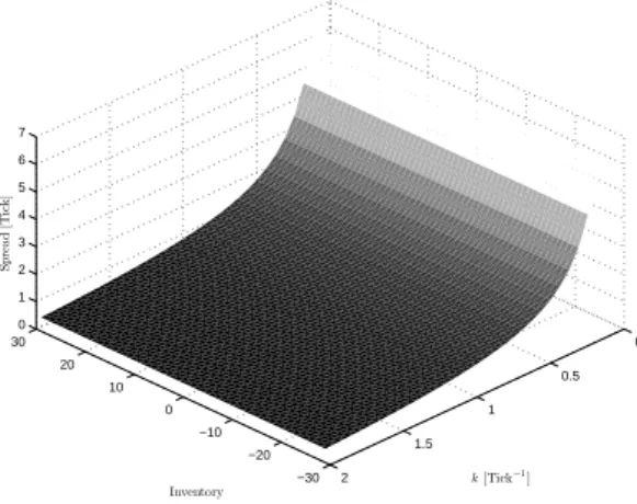
4.3
Dependence on k
From the above approximations we expect δ∞b∗ to be decreasing in k for q greater than some negative threshold. Below this threshold we expect it to be increasing. Similarly we expect
δa∞∗ to be decreasing in k for q smaller than some positive threshold. Above this threshold we expect it to be increasing.
Eventually, as far as the bid-ask spread is concerned, the above approximation indicates that the bid-ask spread should be a decreasing function of k.
∂ψ∞∗ ∂k < 0
In fact several effects are in interaction. On one hand, there is a “no-volatility” effect that is completely orthogonal to any reasoning on the inventory risk: when k increases, trades occur closer to the mid price. For this reason, and in absence of inventory risk, the optimal quotes have to get closer to the mid-price. However, an increase in k also affects the inventory risk since it decreases the probability to be executed (for δb, δa > 0). Hence, an
increase in k is also, in some aspects, similar to a decrease in A. These two effects explain the expected behavior.
Numerically, one of two effects dominates for the values of the inventory under consider-ation: −30 −20 −10 0 10 20 30 0 0.5 1 1.5 2 −1 0 1 2 3 4 5 Inventory k[Tick−1] s− s b [T ic k ] −30 −20 −10 0 10 20 30 0 0.5 1 1.5 2 −1 0 1 2 3 4 5 k[Tick−1] Inventory sa − s [T ic k ]
−30 −20 −10 0 10 20 30 0 0.5 1 1.5 2 0 1 2 3 4 5 6 7 k[Tick−1] Inventory S p re a d [T ic k ]
Figure 5: Asymptotic optimal quotes and bid-ask spread for different inventories and different values of k. σ = 0.3 Tick· s−1/2, A = 0.9 s−1, γ = 0.01 Tick−1, T = 600 s.
4.4
Dependence on γ
Using the above approximations, we see that the dependence on γ is ambiguous. The market maker faces two different risks that contribute to the inventory risk: (i) trades occur at random times and (ii) the mid price is stochastic. But if risk aversion increases, the market maker will mitigate the two risks: (i) he may set his quotes closer to one another to reduce the randomness in execution (as in the “no-volatility” benchmark) and (ii) he may enlarge his spread to reduce price risk. The tension between these two roles played by γ explains the different behaviors we may observe, as in the figures below:
−30 −20 −10 0 10 20 30 0 0.1 0.2 0.3 0.4 0.5 −6 −4 −2 0 2 4 6 8 γ Inventory s − sb [T ic k ] −30 −20 −10 0 10 20 30 0 0.1 0.2 0.3 0.4 0.5 −3 −2 −1 0 1 2 3 4 γ Inventory s − sb [T ic k ] −30 −20 −10 0 10 20 30 0 0.1 0.2 0.3 0.4 0.5 −6 −4 −2 0 2 4 6 8 γ Inventory sa − s [T ic k ] −30 −20 −10 0 10 20 30 0 0.1 0.2 0.3 0.4 0.5 −3 −2 −1 0 1 2 3 4 γ Inventory sa − s [T ic k ]
−30 −20 −10 0 10 20 30 0 0.1 0.2 0.3 0.4 0.5 2 2.5 3 3.5 γ Inventory S p re a d [T ic k ] −30 −20 −10 0 10 20 30 0 0.1 0.2 0.3 0.4 0.5 0.9 0.95 1 1.05 1.1 1.15 1.2 1.25 γ Inventory S p re a d [T ic k ]
Figure 6: Asymptotic optimal quotes and bid-ask spread for different inventories and different val-ues for the risk aversion parameter γ. Left: σ = 0.3 Tick· s−1/2, A = 0.9 s−1, k = 0.3 Tick−1,
T = 600 s. Right: σ = 0.6 Tick· s−1/2, A = 0.9 s−1, k = 0.9 Tick−1, T = 600 s
5
Different settings
In what follows we provide the settings of several variants of the initial model. We will alternatively consider a model with a trend in prices, a model with a penalization term for not having cleared one’s inventory and a model with inventory constraints from which all the figures have been drawn.
For each model, we enounce the associated results and some specific points are proved in the appendix. However, the general proofs are not repeated since they can be derived from adaptations of the proofs of the initial model.
5.1
Trend in prices
In the preceding setting, we supposed that the mid-price of the stock followed a brownian motion. However, we can also build a model in presence of a trend:
dSt= µdt + σdWt
In that case we have the following proposition:
Proposition 3 (Resolution with drift). Let’s consider a family of functions (vq)q∈Z solution
of the linear system of ODEs that follows:
∀q ∈ Z, ˙vq(t) = (αq2− βq)vq(t)− η (vq−1(t) + vq+1(t))
with vq(T ) = 1, where α = k2γσ2, β = kµ and η = A(1 +γk)−(1+
k γ).
Then, optimal quotes can be expressed as: sb∗(t, q, s) = s− ( −1 kln ( vq+1(t) vq(t) ) + 1 γ ln ( 1 +γ k )) sa∗(t, q, s) = s + ( 1 kln ( vq(t) vq−1(t) ) +1 γ ln ( 1 +γ k ))
and the bid-ask spread quoted by the market maker is : ψ∗(t, q) =−1 kln ( vq+1(t)vq−1(t) vq(t)2 ) + 2 γ ln ( 1 +γ k )
Moreover, lim T→∞s− s b∗(0, q, s) = 1 γ ln ( 1 +γ k ) −1 kln ( f0 q+1 f0 q ) lim T→∞s a∗(0, q, s)− s = 1 γ ln ( 1 +γ k ) + 1 kln ( fq0 f0 q−1 ) lim T→∞ψ ∗(0, q) =−1 kln ( fq+10 fq−10 f0 q 2 ) + 2 γ ln ( 1 +γ k )
where f0 ∈ ℓ2(Z) is characterized by:
f0 ∈ argmin ∥f∥ℓ2(Z)=1 ∑ q∈Z α ( q− β 2α )2 fq2+ η∑ q∈Z (fq+1− fq)2
Using the same continuous approximation as in the initial model we find the following approximations for the optimal quotes and the bid-ask spread:
δ∞b∗(q)≃ 1 γ ln ( 1 +γ k ) + [ − µ γσ2 + 2q + 1 2 ] √ σ2γ 2kA ( 1 +γ k )1+kγ δ∞a∗(q)≃ 1 γln ( 1 +γ k ) + [ µ γσ2 − 2q− 1 2 ] √ σ2γ 2kA ( 1 +γ k )1+kγ ψ∞∗ (q)≃ 2 γ ln ( 1 +γ k ) + √ σ2γ 2kA ( 1 +γ k )1+kγ
5.2
Inventory liquidation below mid price
In the initial model we imposed a terminal condition based on the assumption that the market maker liquidates his inventory at mid-price at time t = T . This hypothesis is ques-tionable and we propose to introduce an additional term to model liquidation cost that can also be interpreted as a penalization term for having a non-zero inventory at time T .
From a mathematical perspective it means that the control problem is now: sup
Sa,Sb
E [− exp (−γ(XT + qTST − ϕ(|qT|)))]
where ϕ(·) ≥ 0 is an increasing function with ϕ(0) = 0 that represents the penalization term modeling the incurred cost at the end of the period for not having cleared the inventory6.
The analysis can then be done in the same way as in the initial model and we get the following result:
Proposition 4 (Resolution with inventory liquidation cost). Let’s consider a family of
functions (vq)q∈Z solution of the linear system of ODEs that follows:
∀q ∈ Z, ˙vq(t) = αq2vq(t)− η (vq−1(t) + vq+1(t))
6For analytical reasons we supposed that this penalization term does not depend on S
T. However, nothing
with vq(T ) = e−kϕ(|q|), where α = k2γσ2 and η = A(1 + γk)−(1+
k γ).
Then, optimal quotes can be expressed as: sb∗(t, q, s) = s− ( −1 kln ( vq+1(t) vq(t) ) + 1 γ ln ( 1 +γ k )) sa∗(t, q, s) = s + ( 1 kln ( vq(t) vq−1(t) ) +1 γ ln ( 1 +γ k ))
and the bid-ask spread quoted by the market maker is : ψ∗(t, q) =−1 kln ( vq+1(t)vq−1(t) vq(t)2 ) + 2 γ ln ( 1 +γ k )
Moreover, the asymptotic behavior of the optimal quotes and the bid-ask spread does not depend on the liquidation cost term ϕ(|q|) and is the same as in the initial model.
5.3
Introduction of inventory constraints
Another possible setting is to consider explicitly in the model that the market maker cannot have too large an inventory. This is interesting by itself but it also provides numerical methods to solve the problem and all the graphs presented above have been made using this model that approximates the general one when the inventory limits are large.
5.3.1 The model
In this model, we introduce limits on the inventory. This means that once the agent holds a certain amount Q of shares, he does not propose an ask quote until he sells some of his shares. Symmetrically, once the agent is short of Q shares, he does not short sell anymore before he buys a share.
In modeling terms, it means that the Hamilton-Jacobi-Bellman equation of the problem is the following: ∀q ∈ {−(Q − 1), . . . , 0, . . . , Q − 1}, 0 = ∂tu(t, x, q, s) + 1 2σ 2∂2 ssu(t, x, q, s) + sup sb λb(sb, s) [ u(t, x− sb, q + 1, s)− u(t, x, q, s) ] + sup sa λ a(sa, s) [u(t, x + sa, q− 1, s) − u(t, x, q, s)] for q = Q we have: 0 = ∂tu(t, x, Q, s) + 1 2σ 2∂2 ssu(t, x, Q, s) + sup sa λ a(sa, s) [u(t, x + sa, Q− 1, s) − u(t, x, Q, s)]
and symmetrically, for q =−Q we have: 0 = ∂tu(t, x,−Q, s) + 1 2σ 2∂2 ssu(t, x,−Q, s) + sup sb λb(sb, s) [ u(t, x− sb,−Q + 1, s) − u(t, x, −Q, s) ]
with the final condition:
∀q ∈ {−Q, . . . , 0, . . . , Q}, u(T, x, q, s) = − exp (−γ(x + qs))
As in the initial model we can reduce it to a linear system of ODEs. However the linear system associated to this model will be simpler since it involves 2Q + 1 equations only.
Proposition 5 (Resolution with inventory limits). Let’s introduce the matrix M defined by:
M = αQ2 −η 0 · · · · · · · 0 −η α(Q − 1)2 −η 0 . .. . .. ... 0 . .. . .. ... ... . .. ... .. . . .. . .. ... ... . .. ... .. . . .. . .. ... ... . .. 0 .. . . .. . .. 0 −η α(Q − 1)2 −η 0 · · · · · · · 0 −η αQ2
where α = k2γσ2 and η = A(1 + γk)−(1+γk).
Then, if
v(t) = (v−Q(t), v−Q+1(t), . . . , v0(t), . . . , vQ−1(t), vQ(t))′ = exp(−M(T − t)) × (1, . . . , 1)′
the optimal quotes are:
∀q ∈ {−Q, . . . , 0, . . . , Q − 1}, sb∗(t, q, s) = s− ( −1 kln ( vq+1(t) vq(t) ) + 1 γ ln ( 1 +γ k )) ∀q ∈ {−(Q − 1), . . . , 0, . . . , Q}, sa∗(t, q, s) = s + ( 1 kln ( vq(t) vq−1(t) ) + 1 γ ln ( 1 +γ k ))
and the bid-ask spread quoted by the market maker is given by: ∀q ∈ {−(Q − 1), . . . , 0, . . . , Q − 1}, ψ∗(t, q) =−1 kln ( vq+1(t)vq−1(t) vq(t)2 ) + 2 γ ln ( 1 +γ k )
Moreover, the asymptotic quotes and bid-ask spread can be expressed as:
δb∞∗(q) = 1 γ ln ( 1 +γ k ) − 1 kln ( fq+10 f0 q ) δ∞a∗(q) = 1 γ ln ( 1 +γ k ) +1 kln ( fq0 f0 q−1 ) and ψ∗∞(q) =−1 kln ( fq+10 fq0−1 f0 q2 ) +2 γ ln ( 1 +γ k )
where f0 ∈ R2Q+1 is an eigenvector corresponding to the smallest eigenvalue of M .
5.3.2 Application to numerical resolution
This model based on a slight modification of the initial one leads to a system of linear ODEs whose associated matrix is solely tridiagonal. Hence, for all numerical resolutions we con-sidered this modified problem with the inventory limit Q large enough and the numerical resolution simply boiled down to exponentiate a tridiagonal matrix. The rationale behind
for all times. Since the solution of the initial problem is in ℓ2(Z) for t < T , this approxima-tion will be valid when Q is large as long as t is far enough from the terminal time T and q not too close to Q.
Another possible method is to compute an eigenvector associated to the smallest eigen-value of M . As we noticed before, we expect fq0 to behave as exp
( −1 2 √ α ηq 2).
Hence it’s a better idea to look for g0 instead of f0 where g0q = fq0exp ( 1 2 √ α ηq2 ) . To this purpose, we replace the spectral analysis of M by the spectral analysis of the tridiagonal matrix DM D−1 where D is a diagonal matrix whose terms are
( exp ( 1 2 √ α ηq 2)) q∈{−Q,...,Q}
and g0 will be an eigenvector associated to the smallest eigenvalue of DM D−1.
Now, once g0 has been calculated, the asymptotic values of the optimal quotes and the bid-ask spread are:
δ∞b∗(q) = 1 γ ln ( 1 +γ k ) − 1 kln ( g0 q+1 g0 q ) + 1 2k √ α η(2q + 1) δa∞∗(q) = 1 γ ln ( 1 +γ k ) +1 kln ( gq0 gq0−1 ) − 1 2k √ α η(2q− 1) and ψ∗∞(q) = 2 γln ( 1 +γ k ) − 1 kln ( g0q+1g0q−1 g0 q 2 ) + 1 k √ α η
6
Discussion on the model
6.1
Exogenous nature of prices
In our model, the mid-price is modeled by a brownian motion independent of the behavior of the agent. Since we are modeling a single market maker who operates through limit orders, it seems natural to consider the price process exogenous in the medium run. However, even if we neglect the impact of our market maker on the market, the very notion of mid-price must be clarified. Indeed, one may consider that, although it has little impact on the mar-ket, the market maker can put an order inside the bid-ask spread of the market order book and hence change the mid-price. This would be a misunderstanding of the model since the mid-price is to be considered in the model before any insertion of an order. Hence, the mid-price in this model must be understood as the mid-price of an order book in which our market maker’s orders would be removed. More generally, it may be viewed as a generalized mid-price calculated across trading facilities or any reference price for which the hypothesis on orders arrival is a good approximation of reality.
6.2
Dependence on price
What may be counterintuitive at first sight is that the bid-ask spread or any of the two spreads between quoted prices and market mid-price seems not to depend on the mid-price itself. In fact, in our model, the bid-ask spread and the gap between quoted prices and the market mid-price depends on price, though indirectly, through parameters. Prices are indeed hidden in the trading intensity λ, and more specifically into the parameter k. We indeed considered a trading intensity depending on the distance between the quoted prices and the mid-price. Thus, k must depend indirectly on prices to normalize prices differences.
6.3
Constant size of orders
Another apparent issue of the model is that market makers set orders of size 1 at all times. A first remark is that, if this is an issue, it is only limited to the fact that orders are of constant size since we can consider that the unitary orders stand for orders of constant size
δq or equivalently, though more abstractly, orders of size 1 on a bunch of δq stocks.
If all the orders are of size δq then the stochastic process representing cash is:
d ˜Xt= δq(StadNta− StbdNtb) = δq× dXt
where the jump processes model the event of being hit by an aggressive order (of size δq). Then, if we consider that an order of size δq is a unitary order on a bunch of δq stocks, we can write ˜qt= δq× qt and the optimization criterion becomes:
sup Sa,Sb E[− exp(−γ( ˜XT + ˜qTST) )] = sup Sa,Sb E [− exp (−γδq(XT + qTST))]
Hence, we can solve the problem for orders of size δq using a modified risk aversion, namely solving the problem for unitary orders, with γ multiplied by δq.
However, if we can transform the problem with orders of constant size δq into the ini-tial problem where δq = 1, the parameters must be adjusted in accordance with the fact that orders are of size δq. As such, it must be noticed that A has to be estimated to take account of the expected proportion of an order of size δq filled by a single trade and approx-imations must be made to take account of market making with orders of constant size. In fact, we can consider that, after each trade that partially filled the order, the market maker sends a new order so that the total size of his orders is δq, using a convex combination of the model recommendations for the price7, since in that case the inventory is not a multiple of δq. In our view, this issue is important but it should not be considered a problem to describe qualitative market maker’s behavior and appropriate approximation on A allows us to believe that the error made, as far as quantitative modeling results are concerned, is relatively small.
6.4
Constant parameters
Another issue is that the parameters σ, A and k are constant. While models can be devel-oped to take account of deterministic or stochastic variations of the parameters, the most important point is to take account of the links between the different parameters. σ, A and
k should not indeed be considered independent of one another since, for instance, an
in-crease in A should induce an inin-crease in the number of trades and hence an inin-crease in price volatility.
Some attempts have been made in this direction to model the link between volatility and trades intensity. Hawkes processes (see [6]) for instance may provide good modeling per-spectives to link the parameters but this has been left aside for future work.
7
Applications
In spite of the limitations discussed above we used this model to backtest the strategy on real data. We rapidly discuss the change that have to be made to the model and the way backtests have been carried out. Then we present the result on the French stock AXA.
7.1
Empirical use
Before using the above model in reality, we need to discuss some features of the model that need to be adapted before any backtest is possible.
First of all, the model is continuous in both time and space while the real control problem under scrutiny is intrinsically discrete in space, because of the tick size, and in time, because orders have a certain priority and changing position too often reduces the actual chance to be reached by a market order. Hence, the model has to be reinterpreted in a discrete way. In terms of prices, quotes must not be between two ticks and we decided to ceil or floor the optimal quotes with probabilities that depend on the respective proximity to the neighboring quotes. In terms of time, an order is sent to the market and is not canceled nor modified for a given period ∆t (say 20 or 60 seconds), unless a trade occurs and, though perhaps partially, fills one of the market maker’s orders. Now, when a trade occurs and changes the inventory or when an order stayed in the order book for longer than ∆t, then the optimal quotes on both sides are updated and, if necessary, new orders are inserted.
Now, concerning the parameters, σ, A and k can be calibrated easily on trade-by-trade limit order book data while γ has to be chosen. However, it is well known by practitioners that
A and k have to depend at least on the actual market bid-ask spread. Since we do not
explicitly take into account the underlying market, there is no market bid-ask spread in the model. Thus, we simply chose to calibrate k and A as functions of the market bid-ask spread, making then an off-model hypothesis.
Turning to the backtests, they were carried out with trade-by-trade data and we assumed that our orders were entirely filled when a trade occurred above (resp. below) the ask (resp. bid) price quoted by the market maker.
7.2
Results
To present the results, we chose to illustrate the case of the French stock AXA on November 2nd 2010.
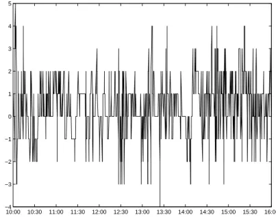
We first show the evolution of the inventory and we see that this inventory mean-reverts around 0. 10:00 10:30 11:00 11:30 12:00 12:30 13:00 13:30 14:00 14:30 15:00 15:30 16:00 −4 −3 −2 −1 0 1 2 3 4 5
Figure 7: Inventory when the strategy is used on AXA (02/11/2010) from 10:00 to 16:00 with
Now, to better understand the very nature of the strategy, we focused on a subperiod of 20 minutes and we plotted the state of the market both with the quotes of the market maker. Trades occurrences involving the market maker are signalled and we can see on the following plot the corresponding evolution of the inventory.
12:30 12:32 12:34 12:36 12:38 12:40 12:42 12:44 12:46 12:48 12:50 13.2 13.21 13.22 13.23 13.24 13.25 13.26 13.27 13.28
Figure 8: Details for the quotes and trades when the strategy is used on AXA (02/11/2010) with
γ = 0.05 Tick−1. Thin lines represent the market while bold lines represent the quotes of the market maker. Dotted lines are associated to the bid side while plain lines are associated to the ask side. Black points represent trades in which the market maker is involved.
12:30 12:32 12:34 12:36 12:38 12:40 12:42 12:44 12:46 12:48 12:50 −4 −3 −2 −1 0 1 2 3
Figure 9: Details for the inventory when the strategy is used on AXA (02/11/2010) with γ = 0.05 Tick−1
Conclusion
In this paper we presented a model for the optimal quotes of a market maker. Starting with the model by Avellaneda ans Stoikov [5] we introduced a change of variables8 that allows to find semi-explicit expressions for the quotes. Then, we exhibited the asymptotic value of the optimal quotes and argued that the asymptotic values were very good approximations for the quotes even for rather small times. Closed-form approximations were then obtained using spectral arguments. The model is finally backtested on real data and the results are promising.
8In a companion paper (see [14]) we used a change of variables similar to the one introduced above to solve
Appendix
Proof of Proposition 1:
This is the classical PDE representation of a stochastic control problem with jump pro-cesses.
Proof of Proposition 2 and Theorem 2:
Let’s consider a solution (vq)qof (S) and introduce u(t, x, q, s) = − exp (−γ(x + qs)) vq(t)−
γ k. Then: ∂tu + 1 2σ 2∂2 ssu =− γ k ˙vq(t) vq(t) u +γ 2σ2 2 q 2u
Now, concerning the bid quote, we have: sup sb λb(sb, s) [ u(t, x− sb, q + 1, s)− u(t, x, q, s) ] = sup sb Ae−k(s−sb)u(t, x, q, s) [ exp ( γ(sb− s) ) (vq+1(t) vq(t) )−γ k − 1 ]
The first order condition of this problem corresponds to a maximum (because u is nega-tive) and writes:
(k + γ) exp ( γ(sb∗− s) ) (v q+1(t) vq(t) )−γ k = k Hence: s− sb∗=−1 kln ( vq+1(t) vq(t) ) + 1 γ ln ( 1 +γ k ) and sup sb λb(sb, s) [ u(t, x− sb, q + 1, s)− u(t, x, q, s) ] =− γ k + γA exp(−k(s − s b∗))u(t, x, q, s) =− γA k + γ ( 1 +γ k )−k γ vq+1(t) vq(t) u(t, x, q, s) Similarly, sa∗− s = 1 kln ( vq(t) vq−1(t) ) + 1 γ ln ( 1 +γ k ) and sup sa λ a(sa, s) [u(t, x + sa, q− 1, s) − u(t, x, q, s)] =− γ k + γA exp(−k(s a∗− s))u(t, x, q, s) =− γA k + γ ( 1 +γ k )−k γ vq−1(t) vq(t) u(t, x, q, s)
Hence, putting the three terms together we get: ∂tu(t, x, q, s) + 1 2σ 2∂2 ssu(t, x, q, s) + sup sb λb(sb, s) [ u(t, x− sb, q + 1, s)− u(t, x, q, s) ] + sup sa λ a(sa, s) [u(t, x + sa, q− 1, s) − u(t, x, q, s)] =−γ k ˙vq(t) vq(t) u +γ 2σ2 2 q 2u− γA k + γ ( 1 +γ k )k γ [ vq+1(t) vq(t) + vq−1(t) vq(t) ] u =−γ k u vq(t) [ ˙vq(t)− kγσ2 2 q 2v q(t) + A ( 1 +γ k )−(1+kγ ) (vq+1(t) + vq−1(t)) ] = 0 Now, noticing that the terminal condition for vqis consistent with the terminal condition
for u, we get that u verifies (HJB).
Proof of Theorem 1 and Theorem 3:
Before starting the very proof, let’s introduce the necessary functional framework. Let’s introduce H =
{
u∈ ℓ2(Z),∑q∈Zαq2u2q+ η(uq+1− uq)2< +∞
}
. H is a Hilbert space equipped with the scalar product:
⟨v, w⟩H =
∑
q∈Z
αq2vqwq+ η(vq+1− vq)(wq+1− wq),∀v, w ∈ H
The first preliminary lemma indicates that the ℓ2(Z)-norm can be controlled by the H-norm. Lemma 1. ∃C > 0, ∀w ∈ H, ∥w∥ℓ2(Z)≤ C∥w∥H Proof: ∀w ∈ H, ∥w∥2 ℓ2(Z) =|w0|2+ ∑ q∈Z∗ |wq|2 ≤ |w0|2+ 1 α∥w∥ 2 H ≤ (|w1| + |w0− w1|)2+ 1 α∥w∥ 2 H ≤ (√1 α + √ 1 η )2 + 1 α ∥w∥2 H
A second result that is central in the proof of our results is that H is compactly embedded in ℓ2(Z).
Proof:
To prove the result we consider a bounded sequence (sk)k∈N in HN. For each k∈ N we
introduce ˆsk defined by:
ˆ
sk0 = sk0, ∀q ∈ Z∗, ˆskq = qskq
For (sk)k∈N is a bounded sequence in HN, (ˆsk)k∈N is a bounded sequence in ℓ2(Z)N. Hence,
we can find ˆs∞ ∈ ℓ2(Z) so that there exists a subsequence indexed by (kj)j∈N such that
(ˆskj)
j∈N weakly converges toward ˆs∞ in ℓ2(Z).
Now, we can define s∞∈ H by the inverse transformation:
s∞0 = ˆs∞0 , ∀q ∈ Z∗, s∞q = 1
qsˆ
∞ q
and it is easy to check that (skj)
N converges in the ℓ2(Z) sense toward s∞. Indeed,
∥skj− s∞∥2 ℓ2(Z)≤ |s kj 0 − s∞0 |2+ ∑ q∈Z∗ 1 q2|ˆs kj q − ˆs∞q |2 =|ˆsk0j − ˆs∞0 |2+ ∑ q̸=0,|q|≤N 1 q2|ˆs kj q − ˆs∞q |2+ ∑ |q|>N 1 q2|ˆs kj q − ˆs∞q |2
The first two terms tend to 0 because (ˆskj)
N weakly converges in ℓ2(Z) towards ˆs∞. The
last one can be made smaller than any ϵ > 0 as N becomes large because ∑|q|>N q12 tends
to zero as N tends to infinity and (∥ˆskj− ˆs∞∥
ℓ2(N))j∈N is a bounded sequence.
Now, we are going to consider a linear operator L that is linked to the system (S). L is defined by
L : f ∈ ℓ2(Z) 7→ v ∈ H ⊂ ℓ2(Z) where
∀q ∈ Z, αq2v
q− η(vq+1− 2vq+ vq−1) = fq
We need to prove that L is well-defined and we use the weak formulation of the equation.
Lemma 3. L is a well-defined linear (continuous) operator.
Moreover ∀f ∈ ℓ2(Z), ∀w ∈ H, ⟨Lf, w⟩H =⟨f, w⟩ℓ2(Z)
Proof:
Let’s consider f ∈ ℓ2(Z).
Because of Lemma 1, w ∈ H 7→ ⟨f, w⟩ℓ2(Z) is continuous. Hence, by Riesz representation
Theorem there exists a unique v ∈ H such that ∀w ∈ H, ⟨v, w⟩H =⟨f, w⟩ℓ2(Z).
This equation writes
∀w ∈ H,∑ q∈Z fqwq = ∑ q∈Z αq2vqwq+ η(vq+1− vq)(wq+1− wq) = α∑ q∈Z q2vqwq+ η ∑ q∈Z (vq+1− vq)wq+1− η ∑ q∈Z (vq+1− vq)wq = α∑ q∈Z q2vqwq+ η ∑ q∈Z (vq− vq−1)wq− η ∑ q∈Z (vq+1− vq)wq
This proves∀q ∈ Z, αq2vq− η(vq+1− 2vq+ vq−1) = fq.
Conversely, if ∀q ∈ Z, αq2v
q− η(vq+1 − 2vq + vq−1) = fq, then we have by the same
manipulations as before that:
∀w ∈ H, ⟨v, w⟩H =⟨f, w⟩ℓ2(Z)
Hence L is well-defined, obviously linear and Lf ∈ H. Now, if we take w = Lf we get
⟨Lf, Lf⟩H =⟨f, Lf⟩ℓ2(Z)≤ ∥f∥ℓ2(Z)∥Lf∥ℓ2(Z)≤ C∥f∥ℓ2(Z)∥Lf∥H
so that ∥Lf∥H ≤ C∥f∥ℓ2(Z) and L is hence continuous.
Now, we are able to prove important properties about L.
Lemma 4. L is a positive, compact, self-adjoint operator
Proof:
As far as the positiveness of the operator is concerned we just need to notice that, by definition:
∀f ∈ ℓ2(Z), ⟨Lf, f⟩
ℓ2(Z) =∥Lf∥2H ≥ 0
For compactness, we know that ∥Lf∥H ≤ C∥f∥ℓ2(Z) and Lemma 2 allows to conclude.
Now, we prove that the operator L is self-adjoint. Consider f1, f2 ∈ ℓ2(Z), we have:
⟨f1, Lf2⟩
ℓ2(Z)=⟨Lf1, Lf2⟩H =⟨Lf2, Lf1⟩H =⟨f2, Lf1⟩ℓ2(Z)=⟨Lf1, f2⟩ℓ2(Z)
Now, we can go to the very proof of Theorem 1 and Theorem 3.
Step 1: Spectral decomposition and building of a solution when the terminal condition is in ℓ2(Z).
We know that there exists an orthogonal basis (fk)k∈N of ℓ2(Z) made of eigenvectors of
L (that in fact belongs to H and we can take for instance ||fk||H = 1) and we denote λk> 0
the eigenvalue9 associated to fk (we suppose that the eigenvalues are ordered, λ0 being the largest one). We have:
αq2fqk− η(fq+1k − 2fqk+ fqk−1) = 1
λkf k q
Hence, if we want to solve (S′) that is similar to (S) but with a terminal condition
v(T )∈ ℓ2(Z) instead of v(T ) = 1 (where 1 stands for the sequence equal to 1 for all indices),
classical argument shows that we can search for a solution of the form v(t) =∑k∈Nµk(t)fk.
90 cannot be an eigenvalue. If indeed λk = 0 then∀w ∈ H, ⟨fk, w⟩
ℓ2(Z)=⟨Lfk, w⟩H = 0. But because H is
Since ∀q ∈ Z
˙vq(t) = αq2vq(t)− η (vq−1(t) + vq+1(t))
= αq2vq(t)− η (vq+1(t)− 2vq(t) + vq−1(t))− 2ηvq(t)
We must have dµdtk(t) = (λ1k − 2η)µk(t) and hence, since λk → 0 we can easily define a
solution of (S′) by: v(t) =∑ k∈N ⟨v(T ), fk⟩ ℓ2(Z)exp (( 2η− 1 λk ) (T − t) ) fk
and the solution is in fact in C∞([0, T ], ℓ2(Z)) Step 2: Building of a solution when v(T ) = 1
The first thing to notice is that H ⊂ ℓ1(Z) (indeed, w ∈ H ⇒ (qwq)q∈ ℓ2(Z) ⇒ (wq)q ∈
ℓ1(Z) by Cauchy-Schwarz inequality). Hence, the sequence v(T ) that equals 1 at each index is in H′, the dual of H. As a consequence, to build a solution of (S), we can consider a similar formula: v(t) =∑ k∈N ⟨1, fk⟩ H′,Hexp (( 2η− 1 λk ) (T − t) ) fk Step 3: Uniqueness
Uniqueness follows easily from the ℓ2(Z) analysis. If indeed v(T ) = 0 we see that we must have that
∀k ∈ Z, ⟨fk, ˙v(t)⟩ ℓ2(Z)= d⟨fk, v(t)⟩ℓ2(Z) dt = ( 1 λk − 2η)⟨f k, v(t)⟩ ℓ2(Z) Hence, ∀k ∈ Z, ⟨fk, v(T )⟩ℓ2(Z)= 0 =⇒ ∀k ∈ Z, ∀t ∈ [0, T ], ⟨fk, v(t)⟩ℓ2(Z)= 0 and v = 0. Step 4: Asymptotics
To prove Theorem 3, we will show that the largest eigenvalue λ0 of L is simple and that the associated eigenvector f0 can be chosen so as to be a strictly positive sequence.
If this is true then we have∀q ∈ Z, vq(0) ∼
T→∞⟨1, f 0⟩ H′,Hfq0exp ( (2η−λ10)T ) so that the result is proved with
δ∞b∗(q) = 1 γ ln ( 1 +γ k ) − 1 kln ( fq+10 f0 q ) δ∞a∗(q) = 1 γ ln ( 1 +γ k ) +1 kln ( fq0 f0 q−1 ) and ψ∗∞(q) =−1 kln ( f0 q+1fq0−1 f0 q 2 ) +2 γ ln ( 1 +γ k ) Hence we just need to prove the following lemma:
Lemma 5. The eigenvalue λ0 is simple and any associated eigenvector is of constant sign (in a strict sense).
Proof:
Let’s consider the following characterization of λ0 and ofthe associated eigenvectors (this characterization follows from the spectral decomposition):
1 λ0 =f∈ℓinf2(Z) ∥f∥2 H ∥f∥2 ℓ2(Z) = inf ∥f∥ℓ2(Z)=1 ∥f∥2 H = inf ∥f∥ℓ2(Z)=1 ∑ q∈Z αq2fq2+ η(fq+1− fq)2
Let’s consider f an eigenvector associated to λ0. We have that: ∑ q∈Z αq2|fq|2+ η(|fq+1| − |fq|)2 ≤ ∑ q∈Z αq2fq2+ η(fq+1− fq)2
Hence, since|f| has the same ℓ2(Z)-norm as f, we know that |f| is an eigenvector asso-ciated to λ0.
Now, since αq2|fq| − η(|fq+1| − 2|fq| + |fq−1|) = λ10|fq|, if |fq| = 0 at some point q, we
have −η(|fq+1| + |fq−1|) = 0 and this induces |fq+1| = |fq−1| = 0, and |f| = 0 by immediate
induction. Since f ̸= 0, we must have therefore |f| > 0.
This proves that there exists a strictly positive eigenvector associated to λ0.
Now, if the eigenvalue λ0 were not simple, there would exist an eigenvector g associated
to λ0 with ⟨|f|, g⟩ℓ2(Z) = 0. Hence, there would exist both positive and negative values in
the sequence g. But, in that case, since |g| must also be an eigenvector associated to λ0, we must have equality in the following inequality:
∑ q∈Z αq2|gq|2+ η(|gq+1| − |gq|)2≤ ∑ q∈Z αq2gq2+ η(gq+1− gq)2
In particular, we must have that ||gq+1| − |gq|| = |gq+1− gq|, ∀q. This implies that ∀q,
either gq and gq+1 are of the same sign or at least one of the two terms is equal to 0. Thus,
since g cannot be of constant sign, there must exist ˆq so that gqˆ = 0. But then, because
|g| is also an eigenvector associated to λ0 we have by immediate induction, as above, that
g = 0.
This proves that there is no such g and that the eigenvalue is simple. Step 5: Positiveness
So far, we did not prove that v, the solution of (S) was strictly positive. A rapid way to prove that point is to use a Feynman-Kac-like representation of v. If (qs)s is a continuous
Markov chain on Z with intensities η to jump to immediate neighbors, then we have the following representation for v:
vq(t) =E [ exp ( − ∫ T t (αqs2− 2η)ds) qt= q ] This representation guarantees that v > 0.
This ends the proof of Theorems 1 and 3
Proof of Proposition 3:
(HJB) 0 = ∂tu(t, x, q, s) + µ∂su(t, x, q, s) + 1 2σ 2∂2 ssu(t, x, q, s) + sup sb λb(sb, s) [ u(t, x− sb, q + 1, s)− u(t, x, q, s) ] + sup sa λ a(sa, s) [u(t, x + sa, q− 1, s) − u(t, x, q, s)]
Using the same change of variables as in the proof of Proposition 2, we can consider a family of strictly positive functions (vq)q∈Z is solution of the linear system of ODEs that
follows:
∀q ∈ Z, ˙vq(t) = (αq2− βq)vq(t)− η (vq−1(t) + vq+1(t))
with vq(T ) = 1, α = k2γσ2, β = kµ and η = A(1 + γk)−(1+
k γ).
Then u(t, x, q, s) =− exp (−γ(x + qs)) vq(t)−
γ
k is a solution of (HJB) and the final condition
is satisfied.
Also, as in the proof of Proposition 2, the optimal quotes are given by:
sb∗(t, q, s) = s− ( −1 kln ( vq+1(t) vq(t) ) + 1 γ ln ( 1 +γ k )) sa∗(t, q, s) = s + ( 1 kln ( vq(t) vq−1(t) ) +1 γ ln ( 1 +γ k )) and the bid-ask spread follows straightforwardly.
To prove the counterparts of Theorem 1 and Theorem 3, we have to write: ˙vq(t) = (αq2− βq)vq(t)− η (vq−1(t) + vq+1(t)) = [ α ( q− β 2α )2 vq(t)− η (vq−1(t)− 2vq(t) + vq+1(t)) ] − ( 2η + β 2 4α ) vq(t)
Hence the operator L and the Hilbert space H are modified but the results are the same
mutatis mutandis.
Proof of Proposition 4:
In this setting, the Bellman function is defined by:
u(t, x, q, s) = sup
Sa,SbE [− exp (−γ(XT
+ qTST − ϕ(qT)))| Xt= x, qt= q, St= s]
The (HJB) equation is:
(HJB) 0 = ∂tu(t, x, q, s) + 1 2σ 2∂2 ssu(t, x, q, s) + sup sb λb(sb, s) [ u(t, x− sb, q + 1, s)− u(t, x, q, s) ] + sup sa λ a(sa, s) [u(t, x + sa, q− 1, s) − u(t, x, q, s)]