A novel measure of physiological condition based on multivariate distance
predicts maximal thermogenic capacity and inflammation in a migratory
shorebird
Emmanuel Milota, Alan A. Cohena*, François Vézinab, Deborah M. Buehlerc, Kevin D. Matsond,
Theunis Piersmad,e
aGroupe de recherche PRIMUS, Dept. de Médecine de famille et de médecine d’urgence,
Université de Sherbrooke, CHUS Fleurimont, 3001 12e Ave N, Sherbrooke, QC J1H 5N4,
Canada
bDépartement de biologie, chimie et géographie, Université du Québec à Rimouski, 300 allée des
Ursulines, Rimouski, QC, G5L 3A1, Canada
cOffice of the Vice President, Research and Innovation, University of Toronto, 12 Queen’s Park
Crescent, Toronto, ON, M5S 1S8
dAnimal Ecology Group, Centre for Ecological and Evolutionary Studies, University of
Groningen, Post Box 11103, 9700 CC Groningen, Netherlands
eDepartment of Marine Ecology, NIOZ Royal Netherlands Institute for Sea Research (NIOZ), PO
Box 59, 1790 AB Den Burg, Texel, The Netherlands *Corresponding author:
Alan Cohen
Dept. de Médecine de famille et de médecine d’urgence Université de Sherbrooke, CHUS Fleurimont
3001 12e Avenue Nord, Sherbrooke, Québec, Canada J1H 5N4
Email: [email protected]
Tel.: +1 819 346-1110 ext. 12589
Running title: Multivariate measure of body condition Word count: 7700
Abstract
1. The body condition of free-ranging animals affects their ability to fulfil their vital needs, their response to stress, their decisions, and ultimately their fitness, with important evolutionary consequences. It is thus a key attribute that ecologists commonly aim to measure, but remains poorly defined and difficult to measure. As recently suggested, ideally a measure of condition should reflect the capacity of an organism to maintain the functionality of cellular processes.
2. We propose a method that provides a holistic assessment of condition, allowing us to position individuals along a gradient from a ‘normal/optimal’ to ‘abnormal/suboptimal’ physiological state. To do so, we make use of the joint probability distribution of multiple physiological biomarkers by computing Mahalanobis multivariate distance over a set of biomarkers. We illustrate the potential of this method by applying it to physiological data collected on a migratory bird, the red knot, during a yearlong experiment. In this
experiment, metabolism, immunity, inflammation and other physiological functions were measured on captive birds caught in the wild.
3. We found that birds with a greater Mahalanobis distance had a lower maximal
thermogenic capacity and higher scores of inflammation. Moreover, all biomarkers except one (haematocrit) showed no significant relationship with the same response variables, indicating that Mahalanobis distance captured a signal on condition that was not detected in individual biomarkers.
4. Mahalanobis distance provides a powerful way to measure condition that accounts for its multivariate nature as well as for the integration of physiological functions into complex regulatory networks. As we discuss, this approach should also prove useful to study a
variety of questions in ecophysiology and evolutionary ecology, such as the relationship between physiological dysregulation and environmental quality, the risk of outcomes such as infections or the mechanisms of adaptive phenotypic plasticity or those behind long-term processes like senescence.
Keywords: Calidris canutus, health state, Mahalanobis distance, metabolic rate, multivariate distance, physiological dysregulation, body condition
Introduction
Body condition is an integral part of animal ecology. First, it may be associated with health outcomes such as infections (Navarro et al. 2003; Arsnoe, Ip & Owen 2011) or with processes affecting the general health state, such as senescence (Kirkwood & Austad 2000). Second, within-individual fluctuations in condition may arise from temporal variation in environmental stressors and provide a flexibility to acclimate to a given environment (Piersma & van Gils 2011). Third, among-individual differences in condition may reflect variation in genetic
(Blanckenhorn & Hosken 2003) or habitat quality (Oliva-Paterna, Miñnano & Torralva 2003; Holt, Fuller & Dolman 2013), or arise from life-history trades-offs (Reed et al. 2008) or maternal effects (Hare & Cree 2011). All the above situations will contribute variance in fitness, with potentially important evolutionary consequences. For instance, condition can affect the costs and benefits of individual strategies, such as those related to dispersal, mating, or reproduction, and favours the evolution of condition-dependent strategies (e.g., Chastel, Weimerskirch & Jouventin 1995; Cotton, Small & Pomiankowski 2006; Kisdi, Utz & Gyllenberg 2012), or influence the evolution of phenotypes (e.g., sexual dimorphism and secondary characters, signal characters; Buchanan 2000; Lorch et al. 2003; Bonduriansky 2007).
Despite an abundant literature on these topics, condition remains a poorly defined concept with often-vague references to viability, vigour, resource reserves, performance or other
descriptors (Johnstone, Rands & Evans 2009; Hill 2011). In addition, well-established indicators such as residual mass, reactive oxidative species, haematocrit, or carotenoids (to name a few) may indeed constitute proxies of variable quality to assess condition (Costantini & Møller 2008?). However, implicit to many studies interested in condition are the fundamental concepts of the ‘general health state’ of an individual and the ‘optimal physiology in a given environment’.
In that sense, the proposition of Hill (2011) to define condition as “the relative capacity to maintain optimal functionality of essential cellular processes” is attractive because it relates directly to these concepts. As Hill stated: “To make sense of this concept of condition, researchers need to be able to define the optimal state of body systems […]”.
From that perspective it seems relevant to shift focus away from single components of condition (e.g. energy store, parasite load) toward measures that provide a more holistic
assessment of condition, perhaps a measure of homeostasis (Hill 2011) which would allow us to position individuals along a gradient from a ‘normal’ to ‘abnormal’ state. To achieve this goal one ideally needs an integrated method to measure condition. Physiological biomarkers offer a promising avenue for that purpose. They are generally useful markers precisely because they are integrated in complex physiological regulatory networks for the maintenance of organism homeostasis, where the levels of different markers are not independent (Cohen et al. 2012; Costantini, Monaghan & Metcalfe 2013), and thus give us a window into underlying system function. They can span various functions (e.g., immune, endocrine, circulation, metabolism, ionic balance, etc.), allowing both the inclusion of numerous relevant variables in the assessment of the condition of an individual (sensu Hill 2011) and testing of specific hypotheses relating condition to physiological functions. For instance, they are commonly used in human studies on aging, frailty and relative risk of health outcomes (McClearn 1997; Walston 2005).
Recently, we showed how using the joint probability distribution of multiple biomarkers to assess individuals’ physiological condition predicts mortality and health outcomes in an elderly human population (Cohen et al. 2013). The underlying hypothesis was that clinical outcome risks increased with increasing global physiological dysregulation in humans, and that an abnormal physiological profile would indicate this dysregulation. Likewise, the physiological response of
wild-ranging animals to environmental challenges, including trade-offs (Buehler et al. 2012), may be a system-level property affected by the general condition or health of an individual. Therefore, it seems highly relevant to apply a similar systems biology approach to ecological questions. The idea is to analyse a sufficient number of biomarkers concurrently to recover a signal of the condition of an individual that can then be related to other variables of interest. This approach should also prove useful for studying longitudinal changes within individuals, with potentially important insights to be gained on long-term processes such as acclimation and senescence.
Here we illustrate the potential of this approach by applying it to published biomarker data on a captive flock of a migrant shorebird, the red knot (Calidris canutus). In the wild, this species is exposed to biotic and abiotic conditions that change drastically over the annual cycle and across the geographical areas occupied during breeding (e.g., high arctic tundra), migratory (e.g., open ocean), wintering (e.g., saline mud flats)(Piersma 2007; Buehler & Piersma 2008). Experiments on captive red knots showed that these birds acclimate to seasonal change in temperature by adjusting their thermogenic capacity (Vézina et al. 2007; Vézina, Dekinga & Piersma 2011). They also exhibit seasonal modulations in constitutive immune function, which apparently are tailored to seasonal environmental challenges (Buehler et al. 2008). Here, we further examined whether the general physiological condition of an individual predicted 1) its maximal
thermogenic capacity or ‘summit metabolic rate’ (Msum, i.e., its capacity to respond to cold stress)
and 2) its level of foot inflammation (Fscore) known as ‘bumblefoot’ and likely reflecting infection
by Staphylococcus bacteria. To assess how normal or abnormal a given biomarker profile was, we used Mahalanobis’s multivariate statistical distance (DM; (Mahalanobis 1936; De
distance from the reference population mean (assumed to represent the average or “normal” physiological state). We show that Msum and Fscore change in the direction that we would predict if
DM was negatively associated with condition, as expected.
Methods
Captive animalsPrevious studies by Buehler et al. (2008; 2012) and Vézina et al. (2011) aimed to study how bird physiology and metabolism adjust to changing requirements across the annual cycle by
comparing individuals held in constant vs. variable environments. Adult red knots from the northerly wintering subspecies (C. c. islandica) were caught in 2004 and kept in aviaries at the shorebird facility of Royal Netherlands Institute for Sea Research (NIOZ). The birds were divided into three groups exposed to different temperature treatments: thermoneutral, cold and variable. Temperature for the latter treatment was modulated by natural conditions outside the facility. Birds exposed to the variable and the thermoneutral treatments were further subdivided in two aviaries and those exposed to the cold treatment were kept together. A total of 30 birds were housed in five aviaries (21 females, 9 males, similar sex ratio among aviaries). The artificial photoperiod tracked the seasonal changes in day length for the Northern Netherlands (53° 31’ N, 6° 23’ E). Phenotypic measurements began in February 2005 and were done monthly for a total of 13 months. Details about conditions in captivity, experimental setting and measurements can be found in Vézina et al. (2006; 2011) and Buehler et al. (2008).
Variables used in the current study are shown in Table 1. Since our goal was to illustrate the multivariate distance method to measure condition, biomarkers were selected simply on the basis of their availability from previous studies. Nonetheless, they represent a large range of functional groups. In the original studies they were initially chosen to investigate the relationship between metabolism and thermogenic capacity, to cover a range of protective functions (immune
measures) and to study covariation between markers from different functional groups (Vézina, Dekinga & Piersma 2011; Buehler et al. 2012). Based on Shapiro tests of normality, some variables required log-transformation prior to the main analyses (Table 1). Since Mahalanobis distance cannot be calculated with missing biomarker values, measurements were available for a total of 259 birds-months, a birth-month corresponding to a measurement taken on a specific bird in a given month.
Mahalanobis distance calculation
Mahalanobis distance (DM)(Mahalanobis 1936) is a multivariate distance that can serve to assess
how close or far an individual’s phenotype is from the mean of a reference population (Cohen et
al. 2013). The reference population can be the sample at hand or another population for which
average trait values and the covariation between them are known (see Discussion). The
interpretation of DM depends on the traits entering its calculation. In the present study we used
DM to establish how far the general physiological state of an individual in a given month was
from the population’s average physiology (including repeated measurements for all individuals). Thus, we interpret the measure as a signal of condition or health state. DM analysis requires the
rather strong assumption of a multivariate normal distribution (MVN) of constitutive traits. Whether this assumption holds will depend on the specific traits, their number and their
covariation. A violation of MVN is, however, likely to lead to conservative results, i.e. a noisier signal of an individual’s state (Cohen et al. 2013). DM is given by
(1)
where x is a multivariate observation, μ is the vector of reference population means for each variable, and S is the reference population variance-covariance matrix. When all variables are uncorrelated (i.e. all non-diagonal elements of the covariance matrix are zero) DM reduces to
(2)
where B is the number of variables and μi and σ2(xi) are the mean and variance in the ith variable,
respectively.
The 11 red knot biomarkers (Table 1) were first standardized by subtraction of the mean followed by division by the standard deviation and then entered in the DM calculation. The full set
of observations served as the reference population to compute μ and S. We also calculated the Mahalanobis distance ‘per treatment’ (DM,t) by using the observations on birds exposed to the
same treatment as the focal individual to compute μ and S. This allowed us to control for differences in population mean due to treatment effects. For example, if the variable treatment resulted in a physiology intermediate to the warm and cold treatments, individuals in the warm and cold treatments would have DM scores further from the total population mean (and thus
calculating DM,t for each individual relative to its treatment, we can account for this possibility.
Shapiro tests indicated that log-transformed DM did not depart from normality (P=0.47) and that
and DM,t was marginally normal (P=0.07). In addition to DM and DM,t, which reflect the
short-term physiological state of each individual at a given month, we also calculated the average value per bird across months (DM,avg, DM,t,avg), reflecting among-individual physiological differences
over the whole year.
Statistical models
We investigated the relationship between DM and two response variables, Msum and Fscore, using
Bayesian generalized mixed-effects models. Msum was chosen because of its adaptive
significance, the maximal thermogenic capacity being a major determinant of bird acclimation to changing temperature over the annual cycle, with potentially important fitness consequences.
Fscore was selected because susceptibility to infection is likely to strongly depend on condition.
After the exclusion of missing values – in particular Msum was not measured in July and August to
avoid potential frostbite of blood-filled feather pins (Vézina et al. 2011) – a total of 182 and 259 birds-months were available for Msum and Fscore analyses, respectively. For all models we used the
nested design of Buehler et al. (2008; 2012) and Vézina et al. (2011) by having individuals nested in aviaries nested in treatments. Thus, bird ID and aviary were fitted as random factors, and treatment as a fixed factor. However, the aviary-effect variance was negligible for Msum, with
negative estimates but at the bound of zero and was excluded from the final Msum model. Month
was included as a fixed factor because previous studies showed that red knots in captivity retain the phenotypic variation schedules of wild birds associated with season and migration. We also initially included the interaction between month and treatment (Vézina et al. 2011) but then
removed it as it showed no significant effect on response variables and decreased much the fit of the models. Sex was fitted only for Fscore as it showed no significant effect on Msum in a previous
analysis of the same data (Vézina et al. 2011; confirmed in our preliminary analyses). The four Mahalanobis distance measures presented above were entered in separate models. In addition, to evaluate whether Mahalanobis distance conveys a signal different from that of individual
biomarkers (i.e. on the general physiological state), we also fitted models with the individual biomarkers as covariates, both with Mahalanobis distance included and excluded.
Msum was marginally normally distributed (Shapiro’s W = 0.986, P=0.06; Fig. 1A) and was
modelled as Gaussian. It was shown to be strongly determined by biological clock- and
temperature- driven modulations of the body mass, in particular in pectoral muscles, which affect heat production capacity (Vézina et al. 2011). Red knots also show a mass-independent increase in thermogenic capacity, i.e. not mediated through an increase in muscular mass. Therefore, Msum
models were fitted with and without mass as a covariate to assess whether DM was related to
mass-independent or total Msum, respectively.
Fscore is an ordinal measure of skin inflammation known as bumblefoot and likely originating
from Staphylococcus infection (Thijs Kuiken, pers. comm.). It ranged from 0 (=no lesion) to 6 (=big lesion) with a mean value of 0.74. Since values included more zeros (62%) than expected from a Poisson distribution (Pr(Fscore=0)=48%, where Fscore ~ Po(µ=0.74); Fig. 1B), we fitted a
zero-inflated Poisson (ZIP) model (see Supporting Methods). Since the zero-inflation parameter estimate was very small (see Results), we also fitted a standard Poisson (SP) model and
compared the results from both models. The magnitude of enduring differences among individuals was estimated by the repeatability (R; Supporting Methods). All analyses were conducted in the MCMCGLMM package (Hadfield 2010) for R (R Development Core Team
2012).
Results
Correlation between DM and other variables
Correlations between biomarkers ranged from -0.24 (Lysis vs. MCEc) to 0.68 (Lym vs. Mon; Fig. 2). DM was either uncorrelated or weakly correlated to biomarkers, ranging from -0.12 (with
Lysis) to 0.20 (with Lym; Fig. 2). There was no clear positive or negative association between
DM and any functional group or subgroup of variables. At most, the correlation between DM and
two types of leukocytes, lymphocytes (Lym) and monocytes (Mon), was of similar magnitude. However, DM was not significantly correlated with heterophils (Het) that also belong to this cell
group. Moreover, DM was positively correlated with hemagglutination (Agg) but negatively with
hemolysis (Lys), which are two methodologically and functionally related indices of innate immunity. Interestingly, Agg and Lys were weakly positively correlated (Fig. 2; as previously reported by Buehler et al. (2011)). This is not surprising considering that, while two biomarkers can be positively correlated, they may show different (within-marker) mean-variance
relationships and that the correlation between DM and a biomarker is shaped by this relationship.
Therefore, DM appears to provide information that is relatively independent from that of
individual biomarkers. Finally, DM was weakly correlated with Fscore (r=0.13, P=0.04) but not
with Msum (r=0.02, P=0.80). Further discussion about correlations between biomarkers
themselves, both within- and among- individuals and across months, can be found in Buehler et al. (2012).
Maximal thermogenic capacity model
As previously found by Vézina et al. (2011), birds from the warm treatment tended to have a lower Msum, while among-month variation was significant (Table 2). The group-effect variance,
after correction for treatment, was negligible, with negative estimates but at the bound of zero (Table 2). Monthly measurements of Mahalanobis distance (DM or DM,t) showed no significant
relationship with Msum (Table 2). However, the average value of an individual over the study
period (DM,avg) was negatively associated with Msum, implying a higher maximal thermogenic
capacity of birds exhibiting a physiology closer to the population average. The effect size was important (Table 2): considering the range of observed DM,avg values (0.96 – 1.36), the effect was
between 3.6 and 5.0 times the magnitude of the warm treatment effect, which showed the highest effect size among fixed factors (i.e. months and treatments). Mass had an effect size between one and two times that of DM,avg, accounting for the range of observed values in both traits. Average
Mahalanobis distance per treatment (DM,t,avg) had a similar, albeit somewhat weaker, effect on
Msum than DM,avg (Table 2). When mass was removed from the model, the decreasing trend of
Msum with increasing DM,avg remained of similar, albeit lower, magnitude but was not significant
(estimate: -5.00, HPD: -10.63 – 1.19, P=0.14). This suggests that the effect of DM,avg on Msum is
independent of mass.
In spite of their significant relationships with Msum, DM,avg and DM,t,avg showed relatively wide
Bayesian 95% highest posterior density intervals (HPD). Since these two variables represent average measures per bird (hence constant over the study period), their effect could have been harder to estimate because of the co-fitting of bird ID as a random effect (due to MCMC sampling toggling part of the Msum variation back and forth between DM,avg and bird ID effects).
controlling for the fixed effects (Table 3). Therefore, on top of the Mahalanobis distance, other unmeasured variables contributed to consistent differences among individuals in terms of Msum.
We fitted a model that included all biomarkers and all previous fixed and random effects.
DM,avg was used as the measure of Mahalanobis’distance since it showed the strongest association
with Msum in the above analyses. This model recovered an effect of DM,avg on Msum of similar
magnitude to the model without the biomarkers (estimate: -5.72, HPD: -11.06 – -0.59, P=0.03). Among biomarkers only haematocrit showed a significant positive relationship with Msum
(estimate: 15.63, HPD: 3.12 – 23.10, P=0.006; Supporting Table 1). Considering the range of observed values (0.4 – 0.56), the effect size of haematocrit on Msum was comparable to that of
DM,avg. An identical model but with DM,avg removed led to similar estimates of biomarker effects,
indicating that the effect (or absence of effect) of biomarkers on Msum is independent from that of
DM,avg (Supporting Table 1).
Foot inflammation score model
The probability that Fscore = 0 due to zero-inflation was very small (P=0.003) and both
distributional assumptions (ZIP and SP) led to a very similar picture of the relationship between explanatory variables and foot inflammation (Table 4). Therefore, we do not distinguish between ZIP and SP except when necessary. Treatment, mass and sex showed no significant relationship with Fscore (Table 4). However, Fscore varied substantially from month to month. A peak occurred
in May, when wild birds undertake the spring migration. DM but not DM,avg had a significant
positive effect on Fscore. This result suggests an association between inflammation and the
punctual condition of an individual but not its average condition over the year (Table 4, Fig. 2). Accounting for the observed DM range (0.25 – 1.93), the effect size (calculated on the observed
scale) was between 0.1 and 0.6 times that of the month with the greatest effect size (estimates from the ZIP model). Mahalanobis distance per treatment (DM,t) had a similar, albeit somewhat
smaller, effect than DM (Table 4). Again, the HPDs for DM,avg and DM,avg were wide, especially on
the observed scale (Fig. 3), probably for the reasons discussed above. Average measurements of Mahalanobis distance (DM,avg or DM,t,avg) showed no significant relationship with Fscore with wide
HPDs on each side of zero (Table 4). As for Msum, repeatability of Fscore was high, accounting for
more than 50% of the variance in after controlling for the fixed effects (Table 3). Aviary effect was much smaller (0.05, HPD: 0.01 – 0.54).
Again, we fitted models (ZIP and SP) with all the biomarkers included, this time choosing DM
as the measure of Mahalanobis’distance since it showed the strongest association with Fscore in
previous analyses. This analysis recovered an effect of DM on Fscore of similar magnitude to the
model without the biomarkers. This effect was slightly higher for the ZIP model (estimate: 1.21, HPD: 0.03 – 1.91, P=0.03) than for the SP model (estimate: 0.98, HPD: -0.04 – 1.85, P=0.052). No biomarker except for haematocrit showed a significant relationship with Fscore (Supporting
Table 2). Haematocrit had a marginally negative significant effect in all models (P-value range: 0.048 – 0.154), but this biomarker had a substantially higher effect size than DM, when
accounting for observed values. Identical models with DM excluded led to estimates of biomarker
effects similar to those from models with DM included (Supporting Table 2).
Discussion
In this study, we assessed the condition of each individual in a sample of red knots by calculating the Mahalanobis distance from biomarker data. To our knowledge this is the first attempt to use a
multivariate distance approach for this purpose in a study of wild-ranging animals. The only former application was done in our study on aging in humans (Cohen et al. 2013). In both cases (red knots, humans) higher DM provided a clear signal of worse individual condition, as shown by
its power to predict variables related to health or physiological performance (i.e., thermogenic capacity, inflammation, survival, chronic diseases). Below we first discuss the properties of the method, including interpretation, advantages and limitations. We then illustrate its potential by discussing the insights gained into the adaptive physiology of red knots and by considering prospective applications in ecology.
Mahalanobis distance as a measure of condition
Mahalanobis distance has been used in a broad range of applications including in ecology (e.g., Farber & Kadmon 2003). It is generally more powerful than univariate proxies (e.g., residual mass) to assess condition because 1) it defines condition relative to a reference population, while the absolute value for individual proxies (including biomarkers) can be driven by factors
unrelated to condition (e.g. see the discussion about haematocrit below); 2) it can simultaneously incorporate numerous biomarkers and thus account for the biological integration of regulatory networks for the maintenance of homeostasis. In fact, integration is typically determined from covariance matrices (Tonsor & Scheiner 2007; Klingenberg 2008; Costantini, Monaghan & Metcalfe 2013), just as Mahalanobis distance is.
Our results strongly support the hypothesis that Mahalanobis distance conveys
information about the condition of animals. First, the relationships between DM and DM,avg and
response variables were not driven by specific biomarkers entered in the distance calculation, as we detected the same effect whether or not individual biomarkers were also entered in the
models. Second, all biomarkers except haematocrit (see below) showed no significant
relationship with response variables, indicating that Mahalanobis distance captured a separate signal. Third, Msum and Fscore changed in the direction that we would predict if Mahalanobis
distance was negatively associated with condition. Specifically, birds with a more ‘abnormal’ physiology had a lower maximal thermogenic capacity and a higher susceptibility to infections. Condition may incorporate aspects such as physical damage or parasites (Hill 2011) that are not directly incorporated in our calculation of Mahalanobis distance. However, these aspects should ultimately translate into physiological effects if they reduce the overall condition of an individual, and are thus likely included indirectly.
One potential drawback of our method is that correlations among biomarkers, including those used here, can change with time (Buehler et al. 2012). This may complicate the choice of the reference population, especially if variation in correlations relates to trade-offs expressed at certain times only. Thus, some exploration of how condition changes with different reference populations may be warranted (see below). Another limitation is that Mahalanobis distance assumes a multivariate normal distribution. However, this is likely to make the comparisons of physiological distance among individuals conservative (Cohen et al. 2013).
Biomarker selection
The biomarkers included in our analyses were selected simply on the basis of the availability of measurements. While this may seem arbitrary, if Mahalanobis distance truly conveys a signal on the general condition of an individual, then the same signal should be detectable with many different combinations of biomarkers; our ability to detect a strong signal with whatever variables happened to be available supports this. In addition, if interactions between the physiological
variables are important contributors to condition, then the predictive power of Mahalanobis distance for condition-dependent variables should increase with the number of biomarkers, as found previously with human data (Cohen et al. 2013).
On the other hand, some markers contribute more signal than others (Cohen et al. 2013), and representation of diverse functional groups is likely important, an issue that remains to be investigated. It is possible that in the future a few specific biomarkers will be found that should be included more systematically in Mahalanobis distance calculation. We are currently
investigating these questions with human data.
Field conditions and blood volume limitations for small organisms may make it difficult to collect sufficient biomarker data to calculate DM in some ecological studies. One potential
solution is cell counters or metabolite analysers that can do an array of measurements from one blood sample with no specific training. Moreover, if the selection of the biomarkers themselves is not much of an issue (as discussed above), it may be possible to focus on a number of simple, cheap markers measurable in miniscule quantities of blood (uric acid, glucose, triglycerides, blood cell counts, etc.).
Reference population
Mahalanobis distance was initially developed to identify observations that represented outliers with respect to several possibly correlated variables (Mahalanobis 1936; Penny 1996; De
Maesschalck, Jouan-Rimbaud & Massart 2000). Typically the reference population selected is the whole data set. We followed that usage here, except when calculating Mahalanobis distance per treatment. The latter would be interpreted slightly differently as the condition of an individual
relative to others exposed to the same treatment. Other types of reference populations can also be used. For instance, in some of our research on aging in humans we limit the reference population to younger individuals that are more likely to have a physiology representative of healthy people (unpublished data). In this case, DM may provide a stronger signal about physiological
dysregulation and senescence. Ideally, the results should not be too sensitive to the choice of the reference population (confirmed here when we replaced DM and DM,avg by DM,t and DM,t,avg,
respectively) unless a different interpretation of Mahalanobis distance is sought. For instance, individuals with the greatest fitness in a given environment could serve as a reference about the optimal physiology in that specific environment.
Mahalanobis distance vs. haematocrit
It is noteworthy that haematocrit, an index of erythrocyte concentration that is sometimes used as a measure of condition, was the only biomarker showing a relationship with response variables. Haematocrit relates to oxygen transport capacity (Prats et al. 1996; Fair, Whitaker & Pearson 2007), which was found to increase in birds in winter (Swanson 1990; Swanson 2010). Given the importance of aerobic metabolism in shivering, as well as the increase of Msum in red knots
exposed to cold experimental conditions (Vézina, Dekinga & Piersma 2011), the association between haematocrit and Msum is not surprising. The (marginally significant) negative
relationship between haematocrit and foot inflammation is more difficult to explain and may seem to support the idea that haematocrit provides a signal on condition. However, in this study haematocrit and Mahalanobis distance were uncorrelated and maintained their respective effects on response variables when they were included in the same model, suggesting that they measure two different things. Moreover, the value of haematocrit as a surrogate for condition is contested
(Dawson & Bortolotti 1997; Fair, Whitaker & Pearson 2007). While the reason for its association with inflammation is not clear, it might be mediated by vessel dilation during inflammation (Sun, Jain & Munn 2007).
Insights into red knot physiology
The red knot has become a model to investigate the adaptive basis of physiological flexibility in free-ranging animals (Buehler & Piersma 2008; Piersma & van Gils 2011). The results presented here provide important insights on this topic. Maximal thermogenic capacity (Msum) is a trait of
critical adaptive significance for migratory birds that must balance the costs and benefits of increased resistance to cold stress under changing thermal conditions in their environment throughout the annual cycle. Previous studies showed that red knots can adjust Msum to external
variations in temperature, principally by changing their mass (Vézina et al. 2006; Vézina, Dekinga & Piersma 2011). Our results further suggest that Msum is also determined by stable
differences in condition among birds (DM,avg). This suggests variation in individual quality,
perhaps owing to good genes or developmental circumstances, and should prompt research in that direction.
Historically higher immune assay scores were considered better (Folstad & Karter 1992; Sheldon & Verhulst 1996; Lochmiller & Deerenberg 2000), but this view has been challenged more recently. Higher scores might indicate higher ability to fight pathogens, but could also reflect current infection (Adamo 2004; Horrocks, Matson & Tieleman 2011). In addition, higher scores might also reflect over (maladaptive) investment in immune function. A salient result of our study is that physiological abnormality in either direction (high or low) correlates with infection, providing evidence that moderate, not extreme, physiology is optimal; however, we
have not decomposed Mahalanobis distance to specify whether this is due to abnormal immune variables specifically.
A large portion of the foot score variance was explained at the individual level (independent of Mahalanobis distance). This suggests strong individual differences in susceptibility to infection that are maintained over the year. Perhaps trade-offs between immune and other functions during energy-demanding periods, such as migration or cold exposition (see Buehler et al. 2008), are less costly for these individuals. This is further suggested by the previous observation that some immune measures are positively correlated among- but negatively within- individuals (Buehler et
al. 2008). The hypothesis could be tested more formally by looking at the within-individual
covariance between immune measures and, for instance, thermogenic capacity or morphometrics associated with flight performance, for groups of birds exhibiting low and high variance in DM. It
might also explain why punctual DM was associated with Fscore while average DM,avg need not be,
if the DM – Fscore relationship is mediated more through individual differences in buffering
capacity than through among-individual variation in average condition. This contrasts with the results obtained with Msum, underscoring the importance of considering variation in condition at
both the within- and among- individual levels when investigating the ecological and evolutionary significance of condition.
Applications to ecology and evolution
The red knot example illustrates how a measure of condition based on Mahalanobis distance opens new prospects for research into ecology. First, one may investigate if departure from “physiological normality” reflects some form of dysregulation or frailty modulated by
predicts outcomes such as infections, diseases or death. Second, the approach can provide insights into adaptive phenotypic plasticity or flexibility when fitness data are available. For instance, a testable hypothesis emerging from our results is that thermal acclimation in red knots comes at a fitness cost that depends on individual quality. A related issue is whether abnormal physiology correlates with fitness in a given environment (eg Watt 1992?). Third, a good measure of condition will be crucial for understanding the evolution of costly secondary sexual traits such as ornaments. Fourth, it can be applied to understand how individual
strategies/decisions such as dispersal express evolutionary trades-offs involving condition. In some sense, Mahalanobis distance may correspond to allostatic load (McEwen & Wingfield 2003) and thus may provide a way to test hypotheses about stress and dysregulation in an ecological context (Wingfield et al. 1998).
Another potential application is the computation of DM from biomarkers belonging to specific
functional groups to test more mechanistic hypotheses. For instance, response to oxidative stress is thought to play an important role in self-maintenance, and there is evidence that environmental stressors affect the level of integration in this metabolic system (Ristow et al. 2009; Costantini, Metcalfe & Monaghan 2010; Costantini, Monaghan & Metcalfe 2013). DM could serve to assess
the normality of an individual’s oxidative profile or as a measure of the level of biological integration within oxidative balance systems.
In conclusion, the use of a multivariate statistical distance based on biomarkers provides a more holistic assessment of body condition than univariate proxies because it relates more tightly to homeostasis, general health state or optimal physiology in a given environment, hence to the functionality of essential cellular processes, which likely is an important determinant of fitness. These are probably the aspects that ecologists aim to grasp when they measure condition and we
thus expect the approach to find many applications in future research.
Acknowledgements
We thank Maarten Brugge and Anne Dekinga for taking care of the captive red knots and Bernard Spaans for capturing the birds. AAC is a member of the FQRS-supported Centre de recherche sur le vieillissement (CDRV) and Centre de recherche Étienne Le-Bel and is a funded Research Scholar of the FQRS. This research was supported byNatural Science and Engineering Research Council of Canada (NSERC) grants to AAC, DMB and FV, a CDRV scholarship to EM, the University of Groningen Ubbo Emmius Scholarship, and Schure-Beijerinck-Popping Fonds to DMB, the Netherlands Organization for Scientific Research and the University of Groningen to TP, and operational grants from NIOZ RoyalNetherlands Institute for Sea Research to TP.
Data accessibility
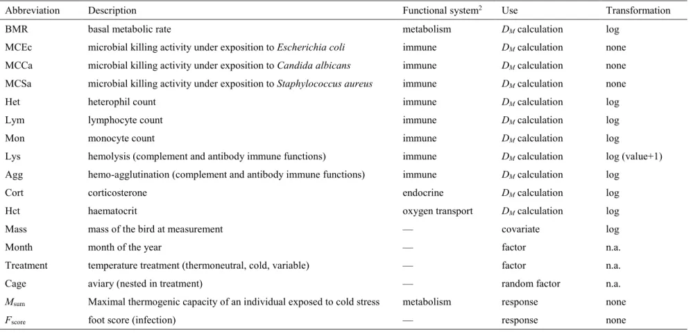
Table 1 Description of the variables used in this study.1
Abbreviation Description Functional system2 Use Transformation
BMR basal metabolic rate metabolism DM calculation log
MCEc microbial killing activity under exposition to Escherichia coli immune DM calculation none
MCCa microbial killing activity under exposition to Candida albicans immune DM calculation none
MCSa microbial killing activity under exposition to Staphylococcus aureus immune DM calculation none
Het heterophil count immune DM calculation log
Lym lymphocyte count immune DM calculation log
Mon monocyte count immune DM calculation log
Lys hemolysis (complement and antibody immune functions) immune DM calculation log (value+1)
Agg hemo-agglutination (complement and antibody immune functions) immune DM calculation log
Cort corticosterone endocrine DM calculation log
Hct haematocrit oxygen transport DM calculation log
Mass mass of the bird at measurement — covariate log
Month month of the year — factor n.a.
Treatment temperature treatment (thermoneutral, cold, variable) — factor n.a.
Cage aviary (nested in treatment) — random factor n.a.
Msum Maximal thermogenic capacity of an individual exposed to cold stress metabolism response none
Fscore foot score (infection) — response none
1Measurements originally done in studies by Buehler et al. (2008, 2012) and Vézina et al. (2011) 2Given for physiological biomarkers only
Table 2 Effect of Mahalanobis distance, mass, treatment and month on the maximal thermogenic capacity (Msum).
Effect size1
Fixed effect (posterior mode) Estimate posterior interval Lower 95% posterior interval Upper 95% probabilityPosterior 2
Mahalanobis distance (DM) -0.44 -1.15 0.20 n.s.
per treatment (DM,t) -0.58 -1.16 0.27 n.s.
average (DM,avg) -6.67 -11.71 -1.60 **
average per treatment (DM,t,avg) -5.17 -10.25 -0.34 *
mass 0.07 0.05 0.09 *** treatment=variable -0.35 -2.00 1.00 n.s. treatment=warm -1.80 -2.94 -0.10 * month=May 2005 -0.90 -1.76 -0.12 * month=June 2005 -1.31 -2.06 -0.70 *** month=September 2005 -1.26 -1.91 -0.47 ** month=October 2005 -1.12 -1.96 -0.59 ** month=November 2005 -1.26 -1.96 -0.61 *** month=December 2005 -1.17 -1.72 -0.36 *** month=January 2006 -1.44 -2.14 -0.84 *** month=February 2006 -1.53 -2.24 -0.94 ***
1Values for treatment, month and mass are those from the model fitted with Dm. Effect sizes from models fitted with
one of the three other Mahalanobis distances were comparable.
Table 3 Repeatability (scale [0,1]) of individual measurements of Msum and Fscore after controlling
for fixed effects (Mahalanobis distance, mass, treatment and month).1
Repeatability Response Distribution modelled Estimate (posterior
mode) posterior interval Lower 95% Upper 95% posterior interval
Msum Gaussian 0.62 0.45 0.75
Fscore zero-inflated Poisson 0.55 0.19 0.78
Fscore Poisson 0.56 0.22 0.87
Table 4 Effect of Mahalanobis distance, mass, treatment and month on foot inflammation (Fscore).
The first value is from the zero-inflated Poisson model and the second (in brackets) from the standard Poisson model.1
Effect size2
Fixed effect (posterior mode) Estimate posterior interval Lower 95% posterior interval Upper 95%
Posterior probability3 Mahalanobis distance (DM) 1.02 (0.87) 0.14 (0.17) 1.83 (1.73) * (*)
per treatment (DM,t) 0.72 (1.01) 0.13 (0.03) 1.92 (1.78) * (*)
average (DM,avg) 0.03 (-0.54) -7.67 (-7.65) 6.67 (7.88) n.s. (n.s.)
average per treatment (DM,t,avg) 0.62 (0.47) -8.80 (-10.23) 6.34 (6.49) n.s. (n.s.)
mass -0.02 (-0.01) -0.03 (-0.03) 0.01 (0.00) n.s. (n.s.) sex 0.33 (-0.23) -1.63 (-1.61) 1.54 (1.62) n.s. (n.s.) treatment=variable 0.68 (0.48) -3.40 (-2.23) 4.00 (3.33) n.s. (n.s.) treatment=warm -0.62 (0.04) -4.12 (-3.46) 3.20 (2.20) n.s. (n.s.) month=May 2005 2.46 (1.73) 0.91 (0.76) 3.63 (3.55) *** (***) month=June 2005 2.13 (1.75) 0.66 (0.73) 3.31 (3.26) *** (**) month=July 2005 1.68 (1.64) 0.63 (0.71) 3.30 (3.27) *** (***) month=August 2005 1.91 (1.59) 0.59 (0.73) 3.25 (3.29) *** (***) month=September 2005 1.76 (1.93) 0.75 (0.84) 3.42 (3.46) *** (***) month=October 2005 2.20 (1.85) 0.86 (0.86) 3.52 (3.28) *** (***) month=November 2005 1.71 (1.51) 0.51 (0.69) 3.22 (3.32) ** (***) month=December 2005 1.18 (1.25) 0.16 (0.23) 2.93 (2.94) * (*) month=January 2006 0.92 (0.75) -0.40 (-0.35) 2.46 (2.60) n.s. (n.s.) month=February 2006 2.01 (1.71) 0.50 (0.72) 3.24 (3.32) *** (***)
1Results from the reduced model without the month×treatment interaction.
2Values for sex, treatment, month and mass are those from the model fitted with Dm. Effect sizes from models fitted
with one of the three other Mahalanobis distances were comparable.
Figure 1 A
B
Figure 1 Distribution of (A) summit metabolic rate and (B) foot scores in from monthly measurements on 30 captive red knots.
Figure 2
Figure 2 Correlation matrix between biomarkers and Mahalanobis distance (DM). The color and
width of the ellipse show the strength of the correlation between two variables (a narrow ellipse indicates stronger correlation) and tilt the direction. An “X” is plotted over the ellipse when the correlation is non-significant (p-value ≥ 0.05). The figure was drawn with the CORRPLOT package
Figure 3
Figure 3 Predicted foot score as a function of Mahalanobis distance (solid line) and 95% Bayesian 95% highest posterior density intervals (dashed lines).
Supplementary Table 1 Effect of individual biomarkers on the maximal thermogenic capacity (Msum). The first value is from the model including DM,avg, i.e. the average Mahalanobis distance
of an individual, and the second (in brackets) is from the model without DM,avg.
Effect size
Biomarker1 (posterior mode) Estimate posterior interval Lower 95% posterior interval Upper 95%
Posterior probability2 BMR -0.41 (-1.09) -2.65 (-2.92) 1.31 (1.23) n.s. (n.s.) MCEc 0.76 (1.13) -0.33 (-0.21) 2.17 (2.31) n.s. (n.s.) MCCa 0.64 (0.48) -0.29 (-0.33) 1.74 (1.71) n.s. (n.s.) MCSa -1.30 (-0.87) -1.94 (-1.99) 0.60 (0.50) n.s. (n.s.) Het 0.00 (0.00) 0.00 (0.00) 0.00 (0.00) n.s. (n.s.) Lym 0.00 (0.00) 0.00 (0.00) 0.00 (0.00) n.s. (n.s.) Mon 0.00 (0.00) 0.00 (0.00) 0.00 (0.00) n.s. (n.s.) Lys 0.03 (0.07) -0.14 (-0.13) 0.25 (0.25) n.s. (n.s.) Agg -0.01 (-0.05) -0.14 (-0.15) 0.10 (0.10) n.s. (n.s.) Cort 0.00 (-0.01) -0.02 (-0.02) 0.00 (0.00) n.s. (n.s.) Hct 15.63 (13.27) 3.12 (3.56) 23.10 (23.10) ** (*)
1See Table 1 for a description of biomarkers
Supplementary Table 2 Effect of individual biomarkers on foot inflammation (Fscore). The first value is from the model including
Mahalanobis distance (DM) and the second (in brackets) from the model without DM.
Zero-inflated Poisson model Standard Poisson model
Effect size Effect size
Biomarker1 Estimate (posterior mode) Lower 95% posterior interval Upper 95% posterior
interval probabilityPosterior 3 (posterior mode) Estimate
Lower 95% posterior
interval
Upper 95% posterior
interval probabilityPosterior 2
BMR -0.03 (-0.84) -2.92 (-2.52) 2.10 (2.34) n.s. (n.s.) -0.08 (-0.33) -2.89 (-2.57) 2.24 (2.33) n.s. (n.s.) MCEc 0.08 (0.14) -1.45 (-1.71) 1.35 (1.21) n.s. (n.s.) -0.05 (-0.38) -1.69 (-1.67) 1.06 (1.14) n.s. (n.s.) MCCa -0.39 (-0.53) -1.48 (-1.51) 0.70 (0.85) n.s. (n.s.) -0.50 (-0.53) -1.55 (-1.68) 0.72 (0.69) n.s. (n.s.) MCSa -0.21 (-0.12) -1.50 (-1.63) 1.18 (1.12) n.s. (n.s.) -0.43 (-0.18) -1.61 (-1.34) 1.25 (1.34) n.s. (n.s.) Het 0.00 (0.00) 0.00 (0.00) 0.00 (0.00) n.s. (n.s.) 0.00 (0.00) 0.00 (0.00) 0.00 (0.00) n.s. (n.s.) Lym 0.00 (0.00) 0.00 (0.00) 0.00 (0.00) n.s. (n.s.) 0.00 (0.00) 0.00 (0.00) 0.00 (0.00) n.s. (n.s.) Mon 0.00 (0.00) 0.00 (0.00) 0.00 (0.00) n.s. (n.s.) 0.00 (0.00) 0.00 (0.00) 0.00 (0.00) n.s. (n.s.) Lys 0.10 (0.11) -0.16 (-0.19) 0.33 (0.33) n.s. (n.s.) 0.04 (0.02) -0.21 (-0.21) 0.29 (0.28) n.s. (n.s.) Agg -0.05 (-0.01) -0.20 (-0.22) 0.13 (0.14) n.s. (n.s.) 0.01 (0.00) -0.16 (-0.15) 0.17 (0.19) n.s. (n.s.) Cort -0.01 (0.00) -0.02 (-0.02) 0.01 (0.01) n.s. (n.s.) -0.01 (0.00) -0.02 (-0.02) 0.01 (0.01) n.s. (n.s.) Hct -6.82 (-10.76) -20.83 (-20.73) 3.27 (2.33) n.s. (n.s.) -10.53 (-11.72) -24.25 (-23.74) 1.44 (0.31) n.s. (*)
1See Table 1 for a description of biomarkers

![Table 3 Repeatability (scale [0,1]) of individual measurements of M sum and F score after controlling](https://thumb-eu.123doks.com/thumbv2/123doknet/2588755.56899/26.918.102.816.157.309/table-repeatability-scale-individual-measurements-sum-score-controlling.webp)
