Incomplete Markets and the Output-Inflation Tradeoff

Incomplete Markets and the Output-In‡ation Tradeo¤

Yann Algan

Edouard Challe

Xavier Ragot

Abstract

This paper analyses the e¤ects of money shocks on macroeconomic aggregates within a ‡exible price, incomplete-markets environment that generates persistent wealth inequalities amongst agents. In this framework, unexpected money shocks redistrib-ute wealth from the cash-rich employed to the cash-poor unemployed and induce the former to increase labour supply in order to maintain their desired levels of consump-tion and precauconsump-tionary savings. The reduced-form dynamics of the model is a textbook ‘output-in‡ation tradeo¤’equation, whereby in‡ation shocks raise current output. The limiting impact of mean in‡ation and money growth persistence on this non neutrality mechanism are also examined.

Keywords: Incomplete markets; borrowing constraints; short-run non-neutrality. JEL codes: E24; E31; E32.

We are particularly grateful to Chris Carroll, Jean-Michel Grandmont, Guy Laroque, Etienne Lehman and Victor Rios-Rull for their suggestions on an earlier version of this paper. We also received helpful comments from seminar participants at CREST-INSEE and participants at the 2007 T2M Conference in Paris. Financial support from the French National Research Agency (ANR) is gratefully acknowledged. All remaining errors are ours.

y_{Paris School of Economics and Paris East University, 48 Boulevard Jourdan, 75014 Paris;}

yann.algan@ens.fr.

z_{CNRS-DRM and Université Paris-Dauphine, 75775 Paris Cedex 16; edouard.challe@dauphine.fr.} x_{Paris School of Economics, 48 Boulevard Jourdan, 75014 Paris; ragot@pse.ens.fr.}

1

Introduction

This paper analyses the e¤ects of money shocks on macroeconomic variables within a ‡exible price, incomplete-markets environment that generates persistent wealth inequalities amongst agents. More speci…cally, we explore the aggregate and welfare e¤ects of unexpected mone-tary injections within a Bewley-type model where money serves as a short-run store of value allowing agents to self-insure against idiosyncratic income ‡uctuations. As was …rst shown by Bewley (1983), and analysed further in a number of contributions including Kehoe et al. (1990), Imrohoroglu (1992), and Akyol (2004), this role for money arises naturally in environments where insurance markets are missing and agents cannot borrow against future income. We draw on this literature by emphasising the role of money as a bu¤er stock against labour income ‡uctuations, where money partly substitutes for the lack of insurance and credit markets. Unlike this existing work, however, we study the short-run non neu-trality of monetary shocks, rather than focusing on the potential long-run, non superneutral e¤ects of steady state in‡ation.

The central result of this paper lies in the derivation of a textbook ‘output-in‡ation tradeo¤’equation, whereby in‡ation shocks contemporaneously raise labour supply and total output. In our economy, in‡ation shocks redistribute wealth from the cash-rich employed (i.e., those who pay the in‡ation tax) to the cash-poor unemployed (i.e., those who bene…t from the in‡ation subsidy), thereby forcing the former to increase their labour supply to replete their income and maintain their desired levels of consumption and money wealth. The implied increase in hours then raises current output, with the underlying tradeo¤ mechanism di¤ering from traditional ones like those based on sticky prices (e.g., Ball et al., 1988) or imperfect information (see Lucas, 1973).

What does the size of this monetary non-neutrality depend on? In our model, the redis-tributive e¤ect of an in‡ation shock is positively related to the gap between the real balances of cash-rich and cash-poor agents, i.e., the degree of inequality in the distribution of money holdings. High mean in‡ation, in as much as it lowers the desirability of real balances as a means of self insurance, tends to deter employed households from accumulating them and thus lowers both money wealth inequalities and the implied impact of in‡ation shocks. Highly persistent money growth shocks, to the extent that they forecast high in‡ation taxes on future real balances, transitorily lowers real money demand and induce a negative e¤ect of

money growth shocks on labour supply and output. Thus, the output e¤ects of in‡ationary money shocks are all the more likely to be large that both the mean and the persistence of money growth are low. In the extreme opposite situation where both are very large, the intertemporal e¤ects on future in‡ation taxes may come to dominate the intratemporal wealth redistribution e¤ect and even lead to a reversal in the slope of the tradeo¤.

Our model follows the route opened by Bewley (1983), Scheinkman and Weiss (1986) and Kehoe et al. (1990). Bewley and Kehoe et al. focused on the optimal long-run in‡ation rate and did not analyse the short-run non-neutrality of money under incomplete markets. Scheinkman and Weiss were the …rst to identify the non-neutrality of money shocks when borrowing constraints make cash holdings heterogenous; however, the in…nite-dimensional wealth distribution of their model did not allow them to derive the output-in‡ation tradeo¤, let alone relate its size to the underlying deep parameters of the model such as, unemployment risk mean in‡ation, or the persitence of shocks. Given the lack of tractability of heterogenous-agent models with in…nite-state wealth distributions, an alternative approach to ours is to solve them computationally. However, computational limitations have thus far limited the applicability of these models to the study of optimal steady-state in‡ation, again leaving aside the analysis of the short-run e¤ects of in‡ation shocks (e.g., Imrohoroglu, 1992, and Akyol, 2004). We circumvent this di¢ culty by deriving a closed form solution to the model with a …nite-state wealth distribution and a …nite number of agent types. Finally, our work is related to that of Doepke and Shneider (2006, Section 4), who look at the aggregate e¤ects of wealth redistribution through in‡ation within an overlapping generations model. In their framework, in‡ation episodes transfer wealth from old retirees to young workers, thereby inducing a decrease in labour supply and output in the short and medium run. In contrast, our model features in…nitely-lived agents occasionally hit by borrowing constraints and is able to generate a positive short run relation between in‡ation and ouput.

Section 2 introduces the model and spells out the optimality and market clearing condi-tions in the general case. Section 3 derives a speci…c closed-form equilibrium with four types of agents and two possible levels of real money balances. Section 4 analyses the properties of the short-run output-in‡ation tradeo¤ generated by the model, with particular attention being paid to the role of mean in‡ation and the persistence of shocks in a¤ecting the slope of the tradeo¤.

2

The model

The economy is populated by a large number of …rms, as well as a unit mass of in…nitely-lived households i 2 [0; 1], all interacting in perfectly competitive labour and goods markets. Firms produce output, yt, from labour input, lt, using the CRS technology yt = lt; they

thus adjust labour demand up to the point where the real wage is equal to 1. Households’ behaviour, on the other hand is potentially a¤ected by both the (uninsurable) idiosyncratic income uncertainty that they are facing and the aggregate shock.

2.1

Uncertainty

Individual states. In every period, each household can be either employed or unemployed. We denote by itthe status of household i at date t, where it = 1if the household is employed

and i

t= 0 if the household is unemployed. Households switch randomly between these two

states, with = prob( i_t+1= 1 i_t = 1) and = prob( i_t+1 = 0 i_t = 0); ( ; ) _{2 (0; 1)}2; being the probabilities of staying employed and unemployed, respectively. Given this Markov chain for individual states, the asymptotic unemployment rate is:

U = (1 ) = (2 ) (1)

The history of individual shocks up to date t is denoted et

i, where eti = f i0; ::; itg:

Et₌

f0; 1g ::f0; 1g is the set of all possible histories up to date t, and i

t: Et ! [0; 1]; t =

0; 1; ::: denotes the probability measures of individual histories (for example, i

t(eit) is the

probability of individual history ei

t for agent i at date t). Following convention, we use the

notation ei

t+1 eit to indicate that eit+1 is a possible continuation of eit. Finally, we limit the

ability of households to diversify this idiosyncratic unemployment risk away by assuming that it is uninsurable and that agents cannot borrow against future labour income.

Aggregate states. Money growth shocks are the only source of economy-wide uncertainty that we consider. The history of these shocks up to date t is denoted ht, while Ht is the set

of all possible histories for these shocks up to date t. Let denote the probability measure over histories up to date t: t: Ht! [0; 1]; t = 0; 1; ::: As before, t(ht)is the probability of

history ht and ht+1 ht indicates that ht+1 is a possible continuation of ht.

In every period, a real amount _t(ht) > 0of newly issued money is given symmetrically to

in equilibrium the price level and the in‡ation rate are functions of the history of aggregate states. These are denoted Pt(ht) and t(ht) Pt(ht) =Pt 1(ht 1) 1; respectively.

2.2

Households’behaviour

The household’s instantaneous utility function is u (c) l, where c is consumption, l is labour supply, > 0 a scale parameter, and where u is a C2 function satisfying u0 > 0, u00 < 0 and (c) u00_{(c) c=u}0_{(c) 18c 0(i.e., consumption and leisure are not gross complements).}

Fiat money is the only asset that households can use to smooth consumption. Employed households (i.e., those for whom i

t = 1) choose their labour supply, lit, at the current wage

rate (= 1), while unemployed households (i.e., for whom it= 0) earn no labour income but

a …xed amount of ‘home production’, > 0.1 _{Let M}i

t denote the nominal money holdings of

household i at the end of date t; and mit Mti=Ptthe corresponding real money holdings (by

convention, let us denote Mi

1 the nominal money holdings of household i at the beginning

of date 0). Household i’s problem is to choose the sequences of functions ci t : Ht Et! R+ li t : Ht Et! R+ mi t : Ht Et! R+ 9 > > > = > > > ; t = 0; 1; :::; that maximise 1 X t=0 t X ht2Ht t(ht) X ei t2Et i t e i t u c i t ht; eit l i t ht; eit ;

where _{2 (0; 1) is the discount factor, subject to} Ptcit ht; eit + M i t ht; eit = M i t 1 ht 1; eit 1 + Pt itl i t ht; eit + 1 i t + t(ht) ; (2) ci_t ht; eit ; l i t ht; eit ; M i t ht; eit 0: (3)

Eq. (2) is the nominal budget constraint of household i at date t, while the last inequality in (3) indicates that agents cannot have negative asset holdings. The Lagrangian function

1_{Alternatively, can be interpreted as an unemployment subsidy …nanced through a compulsory lump}

sum contribution e = (1 ) = (1 ) paid by all employed households and ensuring the balance of the unemployment insurance scheme. In this case, steady state labour supply and output are higher than under the home production interpretation (as working households attempt to o¤set the wealth e¤ect of the unemployment contribution), but the behaviour of the stochastic economy is unchanged.

associated with household i’s problem, formulated in real terms, is:2 L = 1 X t=0 t X ht2Ht t(ht) X ei t2Et t e i t 2 6 4 u (ci_t(ht; eit)) lti(ht; eit) + 'it(ht; eit) mit(ht; eit) + i t(ht; eit) mi t 1(ht 1;eit 1) 1+ t(ht) + i tlti(ht; eti) + (1 it) + t(ht) cit(ht; eit) mit(ht; eit) 3 7 5 ; where the Lagrange multipliers i

tand 'itare positive functions de…ned over Ht Et(we check

below that the non-negativity constraints on cit and lti are always satis…ed in the equilibrium

under consideration). From the Kuhn-Tucker theorem, the optimality conditions are, for t = 0; 1; ::: and for all (ht; eit)2 Ht Et;

u0 ci_t ht; eit = i t ht; eit ; (4) i t ht; eit = if i t = 1 and l i t ht; eit = 0 if i t = 0; (5) i t ht; eit ' i t ht; eit = X ht+1 ht t+1(ht+1) X ei t+1 eit i t+1 e i t+1 i t+1 ht+1; eit+1 1 + t+1(ht+1) ; (6) '_t ht; eit mit ht; eit = 0; (7) lim t!1 t u0 ct ht; eit m i t ht; eit = 0: (8)

Eq. (4) de…nes household i’s marginal utility, while Eqs. (5) and (6) are the intratem-poral and intertemintratem-poral optimality conditions, respectively. Eq. (7) states that either the borrowing constraint is binding for household i ('i

t > 0), implying that cash holdings are

zero (mi

t = 0), or the constraint is slack ('it = 0) and the household uses real balances to

smooth consumption over time (mi

t 0). The transversality condition (8) always hold along

the equilibria that we will consider. Note that Eq. (6) can be written more compactly as: u0 ci_t ht; eit = Et u0 _ci t+1 ht+1; eit+1 1 + t+1(ht+1) ! + 'i_t ht; eit : (9)

2.3

Market clearing

Goods market. Equilibrium in the market for goods requires that, at each date and for all histories of aggregate states ht2 Ht; the sum of each type of agent’s consumption be equal

2_{As will become clear below, our choice of using the Lagrangian function, rather than the Bellman}

to total production. Given the production function assumed, total production is simply the sum of individual labour supplies and home production, so that we have:

Z 1 0 i tl i t ht; eit + 1 i t di = Z 1 0 ci_t ht; eit di;

where the summation operatorR is over individual households.

Money market. Let Mt(ht) denote the nominal quantity of money at date t; then

money-market clearing may equally be written as: Mt(ht) =

Z 1 0

M_ti ht; eit di:

Denote real money supply by mt(ht) Mt(ht) =Pt(ht) and the (gross) rate of money

growth by t(ht) Mt(ht) =Mt 1(ht 1). Then, symmetric real money injections can be

written as: t(ht) = Mt(ht) Mt 1(ht 1) Pt(ht) = mt 1(ht 1) ( t(ht) 1) 1 + t(ht) ; (10) while the law of motion for the real quantity of money is:

mt(ht) =

mt 1(ht 1) t(ht)

1 + t(ht)

: (11)

An equilibrium is de…ned by a set of individual consumption sequences, fcit(ht; eit)g 1 t=0,

in-dividual real money holdings sequences, fmi

t(ht; eit)g 1

t=0, individual labour supply sequences,

flti(ht; eit)g 1

t=0, i 2 [0; 1], and aggregate variables, fyt(ht) ; mt(ht) ; t(ht)g 1

t=0, such that the

optimality conditions (4)-(8) hold for every household i and the goods and money markets clear, given the forcing sequence f t(ht)g1_t=0.

3

A closed-form solution

In general, heterogenous-agent models such as that described above generate an in…nite-state distribution of agent types, as all individual characteristics (i.e., agents’ wealth and implied optimal choices) depend on the personal history of every single agent. In this paper, we derive a closed-form solution of the model with a …nite number of household types by considering an equilibrium where the cross-sectional distribution of money wealth is two-state. The derivation involves three steps. First, we conjecture the general shape of the

solution; second, we identify the conditions under which the hypothesised solution results; and third, we set the relevant parameters (the productivity of home production, here) in such a way that these conditions are always ful…lled along the equilibrium under consideration.

3.1

Conjectured equilibrium

We conjecture the existence of an equilibrium along which

'_t ht; eit = 0 if it= 1 and mit ht; eit = 0 if it= 0; (12)

that is, one where no employed household is borrowing-constrained (so that all of them store cash to smooth consumption), while all unemployed households are borrowing-constrained (and thus hold no cash). From here on, we simplify notation by simply using the i-index for variables that depend on individual histories and the t-index for those that depend on aggregate history.

Consider …rst the consumption level of an unemployed household. If this household was employed in the previous period, then from (2) and (12) their current consumption is:

ci_t= mi_{t 1}= (1 + t) + + t (> 0) ; (13)

On the other hand, from (2) the consumption level of unemployed households who were already unemployed in the previous period is identical across such households and given by: cuu_t = _t+ (> 0) : (14) We now turn to employed households. From Eqs. (4) and (5), their consumption level is identical across employed households and independent of aggregate history, i.e.,

ce = u0 1( ) (> 0) : (15) From Eqs. (9) and (12), the intertemporal optimality condition for an employed house-hold is = Et it+1= (1 + t+1) . If this household is employed in the following period,

which occurs with probability , then i

t+1 = (see Eq. (5)). If the household moves into

unemployment in the next period, then from (4) it+1 = u0 cit+1 , where by construction cit+1

is given by Eq. (13). The Euler equation for employed households is thus: = Et 1 + t+1 + (1 ) Et u0 mi t 1 + t+1 + + _t+1 1 1 + t+1 ; (16)

which in turns implies that all employed households wish to hold the same quantity of real balances, denoted met (i.e., 8i 2 [0; 1], it = 1 ) mit = met). We may thus rewrite Eq. (13),

giving the consumption level of unemployed households which were previously employed, as follows:

ceu_t = me_{t 1}= (1 + t) + + t: (17)

The labour supplies of employed households depend on whether they were employed or not in the previous period. Using Eqs. (2) and (15) these are given by, respectively,

l_tee= u0 1( ) + me_t me_{t 1}= (1 + t) t; (18)

lue_t = u0 1( ) + me_{t t}; (19) with Eqs. (28)–(29) below establishing that both lee

t and ltue are positive in equilibrium.

In other words, when all unemployed households are borrowing-constrained and no em-ployed household is, households can be of four di¤erent types, depending only on their current and past employment status, with their personal history before t 1 being irrele-vant. This distributional simpli…cation is essentially the outcome of the joint assumption that all unemployed households liquidate their asset holdings (i.e., it = 0) mit = 0), while

all employed households choose the same levels of consumption and asset holdings thanks to linear labour disutility (i.e., it= 1) mit= met). We denote these four households types ee,

eu, ue and uu, where the …rst and second letters refer to date t 1 and date t employment states, respectively. Since our focus is on the way idiosyncratic unemployment risk a¤ects self-insurance by the employed, we consider the e¤ect of variations in taking U in (1) as given (the implied probability of leaving unemployment is thus = 1 (1 ) (1 U ) =U). We then write the asymptotic shares of households as:

!ee= (1 U ) ; !eu = !ue = (1 ) (1 U ) ; !uu= U (1 ) (1 U ) ; (20) and we abstract from transitional issues regarding the distribution of household types by assuming that the economy starts at this invariant distribution. Given the consumption and labour supply levels of each type of household, goods-market clearing now implies that:

!eelee_t + !uel_tue+ U = (1 U )ce+ !euceu_t + !uucuu_t : (21) In the equilibrium under study, which we assume to prevail from date 0 onwards, unem-ployed households hold no money while all emunem-ployed households hold the real quantity met.

Money-market clearing thus requires that:

(1 U ) me_t = mt: (22)

3.2

Conditions for the closed-form equilibrium to exist

The condition for the distribution just derived to be an equilibrium is that the borrowing constraint never be binding for ee and ue households but always be binding for both uu and eu households. The constraint is not binding for employed households if the latter never wish to borrow. Thus, interior solutions to (16) must always be such that:

me_t 0: (23)

On the other hand, the Lagrange multiplier 'it must be positive when households are

unemployed, so that from (4)-(6) we must have i

t > Et it+1= (1 + t+1). First consider

uu households, whose current consumption is just + _t (see (14)), and thus for whom

i

t = u0( + t). These households remain unemployed with probability , in which case

they will also consume + _t in the following period and thus it+1 = u0 + t+1 : They

leave unemployment with probability 1 and will then consume u0 1_{( ) in the following}

period, so that it+1 = u0(u0 1( )) = . Thus, uu households are borrowing-constrained

whenever: u0( + _t) > Et u0 ₊ t+1 1 + t+1 ! + (1 ) Et 1 + t+1 : (24) We now turn to eu households. Their current consumption is given by Eq. (17), so that

i

t = u0 met 1= (1 + t) + + t ; while, just like uu households, they will be either uu

or ue households in the following period. Thus, eu households are borrowing-constrained whenever: u0 m e t 1 1 + t + + _t > Et u0 + _t+1 1 + t+1 ! + (1 ) Et 1 + t+1 : (25) If (23) holds then (25) is more stringent than (24), so (25) is a su¢ cient condition for both uu and eu households to be borrowing-constrained. We show in the Appendix that when mean in‡ation is non-negative and lies inside a range ( ; +), where 0 < +,

small support. Intuitively, for our equilibrium to exist home production must be su¢ ciently productive to deter unemployed households from saving, whilst at the same time being su¢ ciently unproductive to induce positive precautionary savings by employed households.

4

Incomplete markets and short-run nonneutrality

4.1

An output-in‡ation tradeo¤ equation

We can now derive the solution dynamics of the closed-form equilibrium. Using Eqs. (10), (11), (16) and (22), we can summarise the dynamic behavior of the economy by a single forward-looking equation, i.e.,

me_t = Et me_t+1 t+1 + (1 ) Et me_t+1 t+1 u0 + m e t+1(U + (1 U ) t+1) t+1 : (26) Eq. (26) determines the equilibrium dynamics of real money balances held by employed households, fme

tg, as a function of the (exogenous) money growth sequence f tg.

In order to examine the redistributive e¤ect of in‡ation shocks in isolation, it is convenient to start by focusing on the e¤ect of i.i.d. money growth shocks on aggregates (auto-correlated shocks are introduced in the next Section). From now on, we further assume that mean money growth is positive (i.e., > 0), and that shocks have small bounded support (so that

t 0 8t). Then, in …rst approximation the solution to (26) is the following constant path

for me t:3 me_t = me= 1 + 1 + (1 U ) u 0 1 (1 + ) (1 ) ; (27)

where unindexed variables denote steady state values (all of these are summarised in the Appendix). Two properties of me _{are worth mentioning at this stage. First, m}e _{falls with}

, as lower idiosyncratic unemployment risk reduces employed households’ incentives to self-insure against this risk. Second, under our maintained assumption that (c) 1; me t

falls with : as in‡ation increases, the return to holding real balances decreases and money becomes less valuable as a self-insurance device against idiosyncratic unemployment shocks.4

3_{This can be checked by linearising (26) around steady state real balances and money growth, (m}e_{; ) ;}

and solving the equation obtained forwards. That (c) 1 implies that the equilibrium is unique and non-cyclical, while i.i.d shocks preclude time-variations in real balances.

We can now turn to the e¤ects of in‡ation shocks on the labour supplies of ee and eu agents and on market output. Substituting (10), (22) and (27) into (18)–(19), we obtain:

l_tee= u0 1( ) + meU t= (1 + t) (> 0) ; (28)

lue_t = u0 1( ) + me(1 + U t) = (1 + t) (> 0) ; (29)

Note that ltee rises while luet falls as t increases. After an in‡ation shock, the households

who pay the in‡ation tax in period t are those who hold money at the beginning of period t (ee and eu households), while the households who bene…t from the corresponding in‡ation subsidy are those who do not hold money at the beginning of period t (ue and uu households). Consequently, ee households are hurt by the shock and increase their labour supply to maintain their desired levels of consumption and money wealth, while ue households can a¤ord to work less than they would have had the shock not occurred. Now, substituting (28)–(29) into market output, yt= !eeltee+ !ueluet , we may rewrite the latter as:

yt= (1 U ) u0 1( ) + (1 U ) me

U t+ 1

1 + t

: (30)

Market output increases with current in‡ation (i.e., greater labour supply by ee house-holds dominates the lower supply of ue househouse-holds) provided that +U > 1, or, equivalently from (1), that + > 1 (that is, the ‘average’ persistence in employment status must be su¢ ciently high) For small shocks, the latter equation can be approximated by the following linear ‘ouput-in‡ation tradeo¤’relation:

yt = y + ( t ) ; (31) where = U + 1 (1 + ) (1 + (1 U ) ) u 0 1 (1 + ) (1 ) : (32)

This tradeo¤ equation is reminiscent of those derived by Lucas (1973) or Ball et al. (1988); the underlying mechanism that we emphasise here works very di¤erently, however. In Lucas, agents raise production after an in‡ationary money shock because they cannot

0. Since u0 1_{((1 + ) = (1 ) ) = c}eu _{(see the Appendix), this condition may be written as:}

ceu+ (1 + ) = (1 ) u00(ceu) < 0;

fully disentangle changes in relative prices from variations in the general price level; in Ball et al., the output-in‡ation tradeo¤ naturally arises from nominal rigidities. In contrast, our model features perfect information, fully ‡exible prices, but heterogenous cash balances. Consequently, lump-sum monetary injections redistribute wealth from cash-rich households to cash-poor ones, thereby inducing employed households to alter their labour supplies in order to o¤set the implied wealth e¤ects. Interestingly, the model predicts that higher trend in‡ation lowers the impact of in‡ation shocks on output (i.e., @ =@ < 0), because it lowers money holdings by employed households and thus mitigates the redistributive e¤ects of these shocks. We may thus conclude that this negative relation is perfectly compatible with price ‡exibility, contrary to the claim by Ball et al. (1988) that it supports the hypothesis of nominal rigidities. We summarise the results obtained so far in the following proposition: Proposition 1. Steady state real money holdings by employed households, me, increase with idiosyncratic unemployment risk, 1 , and decrease with mean in‡ation, . With i.i.d. money growth shocks and U + > 1 (or, equivalently, + > 1), in‡ationary shocks raise current output, yt, the e¤ect being stronger the lower is mean in‡ation.

4.2

Persistent money growth shocks

Central to the transmission of monetary shocks here is the rôle, and determinants, of real money holdings held by the employed as a bu¤er against idiosyncratic unemployment risk. Under i.i.d money growth shocks, these holdings are constant over time as they are imme-diately and entirely repleted by employed households (through variations in labour supply) following a shock that redistributes current wealth. Obviously, this simple adjustment to exogenous disturbances is complicated if real money demand is itself a¤ected by the current shock. In our framework, this precisely occurs when money growth shocks display persis-tence; in this case, a relatively high current in‡ation tax on employed households future high future in‡ation taxes, thereby lowering the desirability of money as a means of self-insurance and reducing households’incentives to supply labour to acquire it. This intertemporal e¤ect induced by the current shock thus runs counter the e¤ect induced by intratemporal wealth redistribution, presumably limiting, or even reverting, the e¤ect of money shocks on total labour supply and market output. To illustrate this point, let us now assume that money

growth obeys the following AR(1) process:

t= (1 ) + t 1+ t; (33)

where _{2 (0; 1) and f} tg1_t=0 is a white noise process with mean zero and small bounded

support. Linearising (26) around the steady state, we obtain: ^

me_t = AEt m^et+1 BEt(^t+1) ; (34)

where hated values denote proportional deviations from steady state (e.g., ^me_t = (me_t me) =me) and A, B are the following constants:

A = 1 (1 + ) (1 =c eu_{) (c}eu₎ 1 + 2 (0; 1) ; B = 1 (1 + ) (1 =c eu_{) (c}eu₎ 1 + U 1 + (1 U ) 2 (A; 1) :

Then, iterating (34) forwards under the transversality condition (8), and using (33), gives: ^

me_t = B

1 A ^t; (35)

where B = (1 A ) > 0. Equation (35) summarises the e¤ect of current money growth on current real balances working through changes in expected money growth, both relative to steady state. To the extent that higher-than-steady state money growth forecasts high future money growth (that is, whenever > 0), then it also forecasts high future in‡ation taxes that discourage current real money accumulation. How do such adjustments in the demand for real balances modify the labour supplies of employed households and implied market output? First, use equations (10), (22) and (18)–(19) again to write the market output equation (30) in the following slightly more general form:

yt= (1 U ) u0 1( ) + (1 U ) met

U ( t 1) + 1 t

: (36) Persistent money growth shocks lower me

t (because of the future in‡ation taxes on real

money), but raise (U ( t 1) + 1 ) t1 provided that U + > 1(through

contemporane-ous wealth redistribution). The actual slope of the tradeo¤ thus ultimately depends on the relative strengths of these two e¤ects. Linearising equation (36) and using (35), we obtain the following results.

Proposition 2. Assume that money growth, t, follows an AR(1) process with

autocorrela-tion parameter _{2 (0; 1). Then, the higher , the lowers is the impact of monetary shocks} on output, while a necessary and su¢ cient condition for these shocks to raise output is:

U + 1 U + 1 >

B 1 A

Whether the latter condition holds or not ultimately depends on the deep parameters that enter both sides of the inequality. When _{! 0, the analysis of the previous Section applies} and monetary shocks raise current output (provided that U + 1 > 0). As is increased, the intertemporal e¤ect gains importance and lowers the impact of shocks, possibly (but not necessarily) leading to a reversal in the slope of the tradeo¤ for large values of . Finally, it is straightfoward to show that su¢ ciently high values of mean in‡ation always lead to the violation of this condition, as they tend to mitigate the intratemporal redistributive e¤ects of shocks.

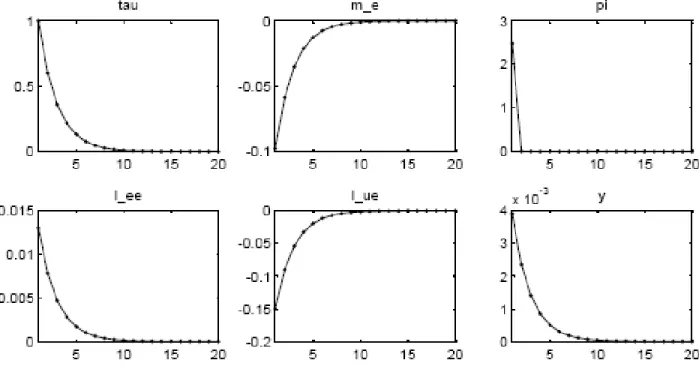
For sake of illustration, Figure 1 displays the dynamic e¤ects of a persitent money growth shock on monetary and aggregate supply variables (…rst and second row, respectively). We set = 0:99, = 0:6, and = 1:005 (the time perid is to be interpreted as a quarter). There are two ways of interpreting U in the context of our model. Strictly speaking, it refers to the unemployment rate. However, the central mechanism underlying the nonneutrality of money here is the redistribution of wealth from cash-rich asset holders to cash-poor, borrowing-constrained agents. Since many real world employed are borrowing-constrained due to low labour income, we interpret U as the share of borrowing-constrained households in the economy and set it to 20%, following Jappelli (1990). We set = 0:95 (so that the share of cash-holding households who will meet the borrowing constraint in the next quarter is 5%) and = 0:9ceu_{. (These parameters ensure that U + > 1, which is necessary for}

money shocks to raise output, and that the existence conditions in Section 3.2 are satis…ed.)

5

Some welfare considerations

Since the nonneutrality mechanism described in this paper relies on wealth redistribution (both at the time of the shock and in the future), it directly a¤ects the welfare of every single agent. Obviously, there potential are loosers and winners resulting from wealth redistribu-tion, meaning that we should not expect monetary shocks to unambiguously lead to better

Figure 1: Dynamic responses to a money growth shock

or worse dynamic equilibria in the Pareto sense. Who gains and who looses following money growth shocks? It may seem at …rst sight that households who bene…t from the in‡ation tax at the time of the shock (uu and ue households, i.e., those who hold no cash at the beginning of the period) always see their utility increase, while those who pay for this tax (ee and eu households, who are cash-rich at the beginning of the period) necessarily experence a welfare loss. But this reasonning is only valid when money growth is i.i.d. but no longer holds when they display auto-correlation. In the latter case indeed, the ongoing transitions of households accross employment status implies that todays’ winners may be tomorrow’s loosers, so that the e¤ect of the current shock on the total expected utility of a particular household is of ambiguous sign.

To understand this point further, note …rst that all time-t variables can be expressed as a function of the only state variable of the model, current money growth t, and that t+1

only depends on t. Call Wi( t) the value function of agent i when current money growth

is t and Wi = @Wi( t) =@ t its (time invariant) …rst derivative. Then, given the transition

derivative of the Bellman equations associated with each agent type gives: Wee = @l ee t @ t + Wee+ (1 ) Weu; Wue = @l ue t @ t + Wee+ (1 ) Weu; Weu = @u (c eu t ) @ t + Wuu+ (1 ) Wue; Wuu = @u (c uu t ) @ t + Wuu+ (1 ) Wue:

The solution to this system expresses the four value function’s …rst derivatives as (cumber-some) functions of @lee

t =@ t; @leet =@ t, @u (ceut ) =@ t, @u (cuut ) =@ t, which themselves depend

on the deep parameters of the model. When = 0 (the limiting i.i.d. case), the welfare responses to the current shock are just given by the responses of households’current labour supplies and consumption demands, and it is then easy to show that Wee _{< 0, W}ue _{> 0,}

Weu _{< 0 and W}uu _{> 0. However, when > 0, one may construct examples where some of}

these signs are reverted. For sake of illustration, compute the limit of Wee _{as = 0:5 and}

! 1 and ! 1 (that is, a situation where currently employed households who pay for the in‡ation tax at the time of the shock are likely to bene…t from it in the future). From the above system, we get:

lim ( ; )!(1;1)W ee₌ 2 2 @lee_t @ t + 1 2 @u (ceu_t ) @ t + 2 1 @u (cuu_t ) @ t :

It is easy to show that @lee

t =@ t is positive but bounded above, that @u (ceut ) =@ t is

negative but bounded below, and that @u (cuut ) =@ tis positive and bounded above. Thus, if

ee-households are su¢ ciently patient (i.e., 2= (1 )is su¢ ciently large), Wee _{reverts sign}

as ( ; ) ! (1; 1) and these households actually bene…t, rather than su¤er, from a positive money growth shock.

Another potentially relevant welfare criterion is the one that would be followed by a benevolent social planner who would give equal weight to every household’s utility. Can this latter one overcome the limitations of the Pareto criterion and yield unambiguous results as to the e¤ects of money growth shocks? To answer this question, …rst use equations (10), (14), (17), (18)–(19) and (22) above to compute the discounted weighted sum of households’

utilities as follows: Wsp( t) = 1 X k=0 t+k X j;l=e;u !jl u(cjl_t+k) ljl_t+k = + 1 X k=0 t+k _!eu_{u c}eu t+k + ! uu_{u c}uu t+k yt+k ;

where is a constant and where the yt+ks terms summarise the welfare losses incurred by

employed agents through higher work e¤ort. Writting the Bellman equation associated with this welfare criterion and taking its derivative with respect to current money growth, we get:

@W_tsp @ t = 1 1 ! eu@u (c eu t ) @ t + !uu@u (c uu t ) @ t @yt @ t :

Here again, we …nd that the sign of @Wtsp=@ t depends on all deep parameters of the

model. Thus, under both criteria the welfare e¤ects of money growth shocks are ambiguous.

6

Conclusion

This papers has uncovered the short-run implications of a simple Bewley-type monetary model with idiosyncratic labour income risk as to the dynamic and welfare e¤ects of monetary shocks. A prerequisite to the derivation of our results was the construction of, and then the focus on, a closed-form equilibrium with limited heterogeneity (both in terms of wealth and agents types) and which may be of independent interest.5 _{We have shown that money growth}

shocks that contemporary redistribute real money wealth across agents tend to raise output, unless this direct e¤ect is conterbalanced by the (indirect) e¤ect of future redistribution on the real demand for cash. Since monetary innovation are in‡ationary (at least at the time of the shock), our model thus tends to generate the positive output-in‡ation relation that has repeatedly been observed in the data. Finally, the fact wealth is redistributed both at the time of the shock and in the future (provided that money growth variations are persistent), combined with the fact that households alternate employment status and thus cash holding levels, implies that the welfare e¤ects of monetary shocks are in general ambiguous.

5_{Kehoe and Levine (2001) have emphasised the inherent di¢ culty of analysing ‘liquidity constrained’}

Bewley models with both indiosyncratic and aggregate uncertainty, due to the very large number of agent types that they typically generate. Our closed-form equilibrium aims to provide a partial answer to this concern.

Appendix A: Steady state of the model

We use variables without time indexation to indicate steady state values. From Eqs. (10)-(11), steady state in‡ation and real transfers are 1 + = (> 1) and = m = (1 + ), respectively. Substituting these values into (16) and using (22), we …nd that steady-state real money holdings by employed households, me_{, are:}

me = 1 +

1 + (1 U ) u

0 1 (1 + )

(1 ) :

The values of cuu_{, c}eu_{, l}ee_{, l}ue _{and y can then be derived straightforwardly. For example,}

ceu = u0 1 (1 + )

(1 ) : (A1)

Since we are considering ‡uctuations occurring arbitrarily close to the steady state, a su¢ cient condition for our closed-form solution to be an equilibrium is that both (23) and (25) hold with strict inequalities in steady state. From (27), the …rst condition is simply:

< u0 1 (1 + )

(1 ) +:

In steady state, the left hand side of (25) is ceu_{. Using (A1), inequality (25) becomes:}

(1 + ) (1 + )

(1 ) (1 ) > u

0_{( + ) : (A2)}

In steady state, = (1 U ) me _{= (1 + ) (see Eqs. (10) and (22)). Substituting into}

(A2), using Eq. (27) and rearranging, we may rewrite the latter inequality as: (1 + ) (1 + ) (1 ) (1 ) > u0 1 + (1 U ) + (1 U ) 1 + (1 U ) u 0 1 (1 + ) (1 ) : (A3) The left-hand side of (A3) is positive at = 0 and thus for all > 0. The right hand side of (A3) is decreasing and continuous in _{over [0; 1). Thus, if (A3) holds when evaluated at} = +, then by continuity there exists < + such that (A3) holds for all > . Setting

= + in (A3) and rearranging, we …nd:

(1 + ) (1 + ) (1 ) (1 ) 2 > 0;

which is always true when > 0 because the left-hand side increases with and is positive at = 0.

References

Akyol, A. (2004), ‘Optimal monetary policy in an economy with incomplete markets and idiosyncratic risk’, Journal of Monetary Economics, 51, pp. 1245-1269.

Ball, L., Mankiw, N.G. and Romer D. (1988), ‘The New Keynesian economics and the output-in‡ation trade-o¤’, Brookings Papers on Economic Activity, 1988(1), pp. 1-82. Bewley, T.F. (1983), ‘A di¢ culty with the optimum quantity of money’, Econometrica, 51(5), pp. 1485-1504.

Doepke, M. and Schneider, M. (2006), ‘Aggregate implications of wealth redistribution: the case of in‡ation’, Journal of the European Economic Association, 4(2-3), pp. 493-502. Imrohoroglu, A. (1992), ‘The welfare cost of in‡ation under imperfect insurance’, Journal of Economic Dynamics and Control, 16, pp.79-91.

Jappelli, T. (1990), ‘Who is credit constrained in the U.S. economy?’, Quarterly Journal of Economics, 105(1), pp. 219-234.

Kehoe, T.J. and Levine, D. (2001), ‘Liquidity constrained markets versus debt constrained markets’, Econometrica, 69(3), pp. 575-598.

Kehoe, T.J. and Levine, D. K. and Woodford, M. (1990). ‘The optimum quantity of money revisited’, Federal Reserve Bank of Minneapolis.Working Papers no 404, July.

Lucas, Jr., R.E. (1973), ‘Some international evidence on output-in‡ation tradeo¤s’, Amer-ican Economic Review Vol. 63, No. 3, pp. 326-334.

Scheinkman, J.A. and Weiss, L. (1986), ‘Borrowing constraints and aggregate economic activity’, Econometrica, 54(1), pp. 23-45.