Financial Flows and the International Monetary
System
∗
Evgenia Passari
Universit´e Paris Dauphine
H´
el`
ene Rey
London Business School, CEPR, NBER
December 18, 2014
Abstract
We review the findings of the literature on the benefits of interna-tional financial flows and find that they are quantitatively elusive. We then present evidence on the existence of a global cycle in gross cross bor-der flows, asset prices and leverage and discuss its impact on monetary policy autonomy across different exchange rate regimes. We focus in par-ticular on the effect of US monetary policy shocks on the UK’s financial conditions.
∗Sargan Lecture, Royal Economic Society (2014). Rey gratefully acknowledges financial
support from the European Research Council (Grant 210584). Email: [email protected].
Passari’ s email: [email protected]. We are very grateful to Elena Gerko, Silvia Miranda-Agrippino, Nicolas Coeurdacier, Pablo Winant, Xinyuan Li, Richard Portes for discussions. We also heartfully thank Peter Karadi and Mark Gertler for sharing their instruments.
1
Introduction
Keynes in the “Economic consequences of peace”, published in 1920 lauded the benefits of international integration in trade and financial flows . He explained how before the first world war “the inhabitant of London could order by tele-phone, sipping his morning tea in bed, the various products of the whole earth, in such quantity as he might see fit, and reasonably expect their early delivery upon his doorstep; he could at the same moment and by the same means ad-venture his wealth in the natural resources and new enterprises of any quarter of the world, and share, without exertion or even trouble, in their prospective fruits and advantages; or he could decide to couple the security of his fortunes with the good faith of the townspeople of any substantial municipality in any continent that fancy or information might recommend.”
After some important setbacks during the wars and the Great Depression, financial openness seems to have resumed its long run upward trajectory. Both emerging markets and advanced economies are increasingly holding large amounts of assets cross border, even though the 2007 crisis has moderated the trend. A simple and widely used measure of de facto financial integration, the sum of cross-border financial claims and liabilities, scaled by annual GDP has risen from about 70% in 1980 to 440% in 2007 for advanced economies, and from about 35% to 70% for emerging markets during the same period (see Lane (2012)). The gross external assets of the UK were 488% and 507% of annual output respectively in 20101.
The menu of assets exchanged across borders has also become broader with derivatives and asset backed mortgage securities becoming internationally traded. It is increasingly important to look at the entire external balance sheet of coun-tries (and not only at net positions) to understand the financial strength and vulnerabilities of countries. As discussed in Gourinchas and Rey (2014), the external assets of the United States for example are tilted towards ”risky as-sets”, equity and FDI which constitute about 49% of total assets between 1970 and 2010, while external US liabilities consist mostly of ”safer assets” such as debt and bank credit. Such heterogeneity in the composition of the balance sheets opens the door to large valuation effects and potentially large wealth transfers across countries (see Gourinchas and Rey 2007 and Gourinchas, Rey and Govillot 2010)who argue that the US plays the role of the world insurer during global crises and Gourinchas, Rey and Truempler (2012) who estimate valuation changes during the 2008 crisis.
The scope for international capital flows to provide welfare gains or losses has therefore increased considerably in recent decades. The academic literature has attempted to measure gains to financial integration mainly in two ways: by testing for growth effects and better risk sharing following financial account opening using either panel data or event studies.and by calibrating standard international macroeconomic models and computing gains when going from au-tarky to financially integrated markets. Perhaps surprisingly, both streams of
literature have so far failed to deliver clear cut results supporting large gains to financial integration. In the international risk sharing literature, there is still a lively debate regarding the gains that can be achieved by diversification of the portfolios (Obstfeld (2009), Van Wincoop (1994,1999), Lewis (1999, 2000), , Coeurdacier and Rey (2013), Lewis and Liu(2014)). In the allocative efficiency literature based on the neoclassical growth model, gains have been found to be relatively small (Gourinchas and Jeanne (2006)), Coeurdacier, Rey and Winant (2014). Recent surveys of the empirical literature such as Jeanne et al (2012) tend to conclude that there is little support in the data for gains from financial integration.
On the other hand, some costs to integration, due in particular to mone-tary policy spillovers have become more apparent with the recent crisis. The international finance literature has often used the framework of the Mundel-lian “trilemma”: in a financially integrated world, fixed exchange rates export the monetary policy of the base country to the periphery. The corollary is that if there are free capital flows, it is possible to have independent monetary policies only by having the exchange rate float; and conversely, that floating exchange rates enable monetary policy independence (see e.g. Obstfeld and Taylor (2004)). But does the current scale of financial integration put even this into question? Are the monetary conditions of the main world financing cen-tres, in particular the United States, setting the tone globally, regardless of the exchange-rate regime of countries?
In the second section of the paper we discuss the sources of potential gains from financial integration and will assess their magnitude in the context of the textbook neoclassical growth model. In the third part, we discuss the costs of financial integration in the form of loss of monetary policy autonomy. We show the existence of a global financial cycle and discuss its characteristics. In a fourth part, we then investigate in more details whether the exchange rate regime alters the transmission of financing conditions and monetary policy shocks. In the last part we analyse the effect of US monetary policy on the global financial cycle and explore empirically whether a flexible exchange rate regime (the one of the United Kingdom) insulates countries from US monetary policy shocks.
2
Welfare benefits of financial capital flows
The welfare benefits of financial integration is one of the long standing issues in international finance. The neoclassical growth model is behind many of our economic intuitions regarding why the free flow of capital could be beneficial. Within this model, financial integration brings improvements in allocative ef-ficiency as capital flows to places with the highest marginal product, which is the capital scarce economy. As explained in Gourinchas and Rey (2014), those countries are characterised with a high autarky rate of interest compared to the world interest rate. Emerging markets, which tend to be more capital scarce than mature OECD economies, should hence benefit from financial integration as imported capital enables them to consume and invest at a faster pace than
if they had remained in financial autarky.
It is only recently (see Gourinchas and Jeanne (2006)) that the welfare gains of going from autarky to a world where a riskless bond can be traded interna-tionally have been evaluated quantitatively in the textbook deterministic neo-classical growth model. Interestingly those welfare gains have been found to be small: they are worth a few tenths of a percent of permanent consumption for a small open economy even if it starts with a relatively high level of capital scarcity (calibrated to match the actual capital scarcity of emerging markets). The reason is that financial integration enables an economy to speed up its transition towards its steady-state capital stock but that does not bring large welfare gains as the distortion induced by a lack of capital mobility is transi-tory: the country would have reached its steady-state level of capital regardless of financial openness, albeit at a slower speed. In this framework, only very capital-scarce countries could possibly experience significant gains to financial integration.
Figure 1, taken from the analysis of Coeurdacier, Rey and Winant (2014) illustrates the time paths of consumption and capital for an emerging market which is capital scarce and a developed economy whose capital stock is already at its steady state. Otherwise the environment is fully symmetric and there is no uncertainty. Dotted lines denote the autarky states while continuous lines denote the paths after financial integration (a riskless bond can be traded in-ternationally). Time is measured in years on the horizontal axis. The economy is a deterministic two-country neo classical growth model (for details on the model and calibration see Coeurdacier et al. (2014)). The upper right panel shows that the time path of capital accumulation for the emerging market, when there is financial integration, is above the autarky path in the transition period before it reaches its steady state level. The steady state level of capital is the same under financial integration and under autarky2. The gains to financial
integration are thus limited to the area between the two curves and turn out to be quantitatively quite small. The developed country gains from financial inte-gration, but also quantitatively in a very small way. As shown in the lower right panel, it starts by exporting capital to the emerging market (thus accumulating net claims on the emerging markets). Hence the consumption of the emerging market (upper left panel) is at first above its autarky level but then beneath it as it needs to repay its liabilities to the mature economy. The mirror image is true for the advanced economy which benefits in the long run from a higher consumption level than under autarky (lower left panel). The world interest rate establishes itself in between the two autarky rates of interest.
When calibrated to standard values used in the literature, the welfare gains are found to be small, of the order of a few tenths of a percent of permanent consumption. They are even smaller than in the Gourinchas and Jeanne (2006) small open economy paper as a general equilibrium effect via movements in the world rate tends to dampen welfare gains: the emerging market welfare is
2As analysed in Coeurdacier et al. (2014), this is no longer true in a stochastic world with
negatively affected by the world interest rate going up following integration, as it is a net debtor to the rest of the world.
The model described here however is deterministic (as in Gourinchas and Jeanne (2006)) and cannot therefore be used to analyse the welfare gains linked to international risk sharing. Financial integration enables better risk sharing, as long as countries idiosyncratic risks are not perfectly positively correlated. Coeurdacier et al. (2014) are the first ones to analyse welfare gains in a more general neo classical growth model in a stochastic setting, allowing for asym-metries in risk and capital scarcity. They show that gains from increased al-locative efficiency and from risk sharing are intertwined in interesting ways and that they can generate very rich and non monotonic patterns of international capital flows over time. Their model can for example generate global imbalances (capital flowing from the emerging market to the developed economy) without any additional friction. They conclude however that welfare gains of financial integration remain relatively small even in that broader setting and even when they consider models with realistic risk premia.
[FIGURE 1 ABOUT HERE]
Figure 1: Consumption and Capital for an Emerging Market and a Developed Economy (Coeurdacier, Rey and Winant (2011))
There are other channels through which financial integration could be ben-eficial. It could have direct effects on Total Factor Productivity via financial
markets development or institutional changes. It could discipline macroeco-nomic policies. We still lack convincing empirical evidence on these channels however (see the survey of Jeanne et al (2012)), which constitute an interesting agenda for further research. Since the large empirical literature on financial in-tegration is still inconclusive as well, at this stage, one can therefore summarize our view by stating that large gains from financial integration cannot be taken for granted.
3
Financial Integration and the Global
Finan-cial Cycle
Some costs to financial integration, due in particular to monetary policy spillovers have become more apparent in the run up of and during the 2007 crisis. The international finance literature has often used the framework of the Mundellian “trilemma” to discuss monetary autonomy. In a world of free capital mobil-ity, fixed exchange rates export the monetary policy of the base country to the periphery. The corollary is that it is possible to have independent monetary policies only by having the exchange rate float; and conversely, that floating ex-change rates enable monetary policy independence (see e.g. Obstfeld and Taylor (2004), Klein and Shambaugh (2013), Goldberg (2013)). But the current scale of financial integration may put even this into question. Monetary conditions of the main world financing centres, in particular the United States, may spill over into many jurisdictions, regardless of the exchange-rate regime of countries. Indeed, the recent period of financial globalization has been characterized by the existence of what Rey (2013) called a ”Global Financial Cycle3”. We now present a few stylized facts that characterize the global financial cycle.
Stylized fact 1:
There is a clear pattern of co-movement of gross capital flows, of leverage of the banking sector, of credit creation and of risky asset prices (stocks, corporate bonds) across countries4. This is the Global Financial Cycle. Rey (2013) shows that gross inflows across geographical areas and across asset classes (credit, portfolio debt and equity, FDI) are overwhelmingly positively correlated.
Stylized fact 2 :
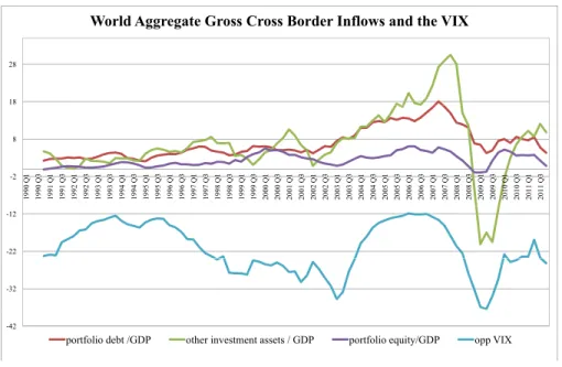
Indices of market fear (such as the VIX, the VSTOXX, the VFTSE or the VNKY5) tend to co-move negatively with gross cross-border flows (see also
3The global financial cycle is related to but is different from the national financial cycles
described by Drehmann, M, C Borio and K Tsatsaronis (2012), who emphasize in particular the cycles in credit and real estate prices.
4For the precise list of countries see Appendix A. For more details on leverage and credit
growth and risky asset prices, see Miranda Agrippino and Rey (2012).
5The VIX is the Chicago Board Options Exchange Market Volatility Index. It is a measure
of the implied volatility of S&P 500 index options. The VSTOXX is the European equivalent, while the VFTSE and the VNKY are the UK and the Japanese equivalents respectively.
Forbes and Warnock (2012)). Figure 2 illustrates comovement of the VIX with world aggregate gross cross border inflows of portfolio debt, equity and credit6. As risk aversion and volatility increase cross border transactions go down.
[FIGURE 2 ABOUT HERE]
World Aggregate Gross Cross Border Inflows and the VIX
18 28 8 -2 1990 Q1 1990 Q3 1991 Q1 1991 Q3 1992 Q1 1992 Q3 1993 Q1 1993 Q3 1994 Q1 1994 Q3 1995 Q1 1995 Q3 1996 Q1 1996 Q3 1997 Q1 1997 Q3 1998 Q1 1998 Q3 1999 Q1 1999 Q3 2000 Q1 2000 Q3 2001 Q1 2001 Q3 2002 Q1 2002 Q3 2003 Q1 2003 Q3 2004 Q1 2004 Q3 2005 Q1 2005 Q3 2006 Q1 2006 Q3 2007 Q1 2007 Q3 2008 Q1 2008 Q3 2009 Q1 2009 Q3 2010 Q1 2010 Q3 2011 Q1 2011 Q3 -22 -12 -32 -42
portfolio debt /GDP other investment assets / GDP portfolio equity/GDP opp VIX
Figure 2: VIX and World Aggregate Gross Cross Border Inflows of Portfolio Debt, Equity and Credit,1990-2012. All variables are quarterly averages
Stylized fact 3 :
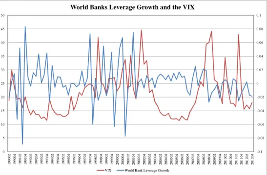
Indices of market fear (such as the VIX, the VSTOXX, the VFTSE or the VNKY) tend to co-move negatively with credit and leverage growth (see also Bruno and Shin (2014)). Figure 3 presents the joint time variations of a world measure of banking leverage broadly defined as loan-to-deposit ratio7and of the
VIX.
6See Appendix B for details on the data
[FIGURE 3 ABOUT HERE] -0 02 0 0.02 0.04 0.06 0.08 0.1 20 25 30 35 40 45 50
World Banks Leverage Growth and the VIX
-0.1 -0.08 -0.06 -0.04 -0.02 0 5 10 15 20 199002 199004 199102 199104 199202 199204 199302 199304 199402 199404 199502 199504 199602 199604 199702 199704 199802 199804 199902 199904 200002 200004 200102 200104 200202 200204 200302 200304 200402 200404 200502 200504 200602 200604 200702 200704 200802 200804 200902 200904 201002 201004 201102 201104 201202 201204
VIX World Bank Leverage Growth
Figure 3: Joint Time Variations of a World Measure of Loan-to-Deposit Ratio and the VIX, 1990-2012
Both measures have been smoothed by taking quarterly averages. The degree of comovement between the two series is striking. It confirms and generalizes the results of Adrian and Shin (2014) who find a significant negative correlation between leverage and the VIX in banks microeconomic data. One possible rationalization of this negative correlation between the VIX and leverage has been provided by Borio and Zhu (2011) and Adrian and Shin (2014) who argue that banks behave like risk neutral value at risk investors but that historical measures of risk lead to procyclical leverage behaviour. In good times, perceived risk is low, spreads are low, value at risk constraints are relaxed which leads to more investment and bids up valuation of assets further. The reverse happens in bad times.
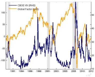
Risky asset prices (equities, corporate bonds) around the world are largely driven by one global factor. This global factor is tightly negatively related to the VIX.
[FIGURE 4 ABOUT HERE]
Figure 3: Global factor and VIX. Source: Miranda‐Agrippino and Rey (2012). To sum up, we have now established in flow data (across most types of flows and regions, but with some exceptions) and in price data (across a sectorally and geographically wide cross‐section of risky asset prices) the existence of a global financial cycle. Interestingly, the VIX is a powerful index of the global financial cycle, whether for flows or for returns. Our analysis so far emphasizes striking correlations and patterns, but cannot address causality issues. Low value of the VIX, in particular for long periods of time, are associated with a build up of the global financial cycle: more capital inflows and outflows, more credit creation, more leverage and higher asset price inflation. III) Capital flows and market sensitivities to the global financial cycle In this part I attempt to gauge further the importance of the global financial cycle for different asset markets (stock prices, house prices) as well as for the leverage of financial intermediaries. Having reported the importance of the global cycle for the fluctuations of these variables in the time series dimension, I study in more details the factors affecting the cross sectional sensitivities of these variables to the global financial cycles. More precisely, I focus here on the possibility that larger
Figure 4: Global Factor and VIX, 1990-2012 (Miranda Agrippino and Rey (2012))
The behaviour of risky assets around the globe is very striking. One might think that prices of equities and corporate bonds reflect to a large extent conti-nent specific, sector specific, country specific and company specific factors. But, as shown by Miranda Agrippino and Rey (2012) using a large cross section of 858 risky asset prices distributed on the five continents, an important part of the variance of risky returns (25%) is explained by one single global factor. This result is remarkable given the size and the heterogeneity of the set of returns. Figure 4 presents the time variation of the single global factor that explains a large part of the variance of the cross section. It increases from the early 1990s until mid 1998, the time of the Russian crisis. From the beginning of 2003, the index increases rapidly until the beginning of the third quarter of 2007. This coincides with the increased vulnerability of the financial markets worldwide and the growing alarms of market participants on the existence of heightened counterparty risk. The high degree of negative correlation of the global factor with the VIX is striking. Building on the analyses of Adrian and Shin (2008)
and Danielsson, Shin and Zygrand (2011) , Miranda-Agrippino and Rey (2012) show that the global factor can be interpreted as reflecting the evolution of two variables:1) the effective risk appetite of the market, defined as the weighted average of risk aversion of leveraged value at risk investors such as global banks and risk averse fund managers such as pension funds; 2) realized world market volatility of traded risky assets. Given that structural interpretation, it may not be surprising that the global factor in asset prices is found empirically to be closely related to the VIX.
In this section we laid out the characteristics of the global financial cycle. There are striking commonalities in movements in credit, leverage, gross flows, risky asset prices across countries. All these variables are found to comove negatively with the VIX and other indices of market volatility and risk aversion. In the next section we investigate whether exchange rate regimes can insulate countries from the global financial cycle.
4
Global Financial cycle and exchange rate regimes
We start by asking whether the positive correlations across inflows into different geographical entities (stylized fact 1, documented in detail in Rey (2013)) are affected by the exchange rate regime of countries. Figure 5 presents a compre-hensive heatmap of capital inflows comprising all asset classes (FDI, portfolio equity, portfolio debt and credit8) into different countries. We have classified the countries by exchange rate regimes, the darker shades corresponding to floating regimes and the lighter shades corresponding to fixed regimes. The data for the flows are quarterly ranging between the first quarter of 1990 and the last quarter of 2012 and come from the IMF International Financial Statistics database. The exchange rate regime data are taken from the update of the monthly de facto exchange rate regime classification of Reinhart and Rogoff (2004) by Ilzetzki and Reinhart (2009) . The exchange rate regime is multilateral; we do not consider bilateral regimes vis-a-vis the US dollar (though that would be an interesting analysis to perform in itself) as monetary policy autonomy is impeded as soon as the exchange rate is not freely floating irrespective of the base currency a country pegs to. Hence, euro area countries have a rigid exchange rate regime for a large part of the sample despite the fact that the euro floats against the US dollar. The Reinhart and Rogoff coarse classification ranges from 1 to 6, the lower numbers corresponding to the more fixed exchange rates with the higher numbers corresponding to free floaters up till 49. We exclude categories
8Technically, bank loans and trade credit.
9In particular, 1 denotes no separate legal tender, a pre announced peg or a currency board
arrangement, a pre announced horizontal band that is narrower than or equal to +/-2% or a de facto peg; 2 stands for announced crawling peg, pre announced crawling band that is narrower than or equal to +/-2%, de facto crawling peg, or de facto crawling band that is narrower than or equal to +/- 2%; 3 denotes pre announced crawling band that is wider than or equal to +/- 2%, de facto crawling band that is narrower than or equal to +/-5%, moving band that is narrower than or equal to +/-2% or managed floating currency regime and 4
5 (freely falling currencies) and 6 (dual market in which parallel market data is missing) due to the small number of observations available. Our regime variable therefore takes the values 1,2,3 and 4, where lower values suggest a more rigid regime. The exchange rate regime variable is time varying and we use it as such in the panel regressions below. But for the heatmap we average its value over the sample and use this time series average value to rank our countries according to the degree of rigidity of their exchange rate regime. The heatmap thus presents the correlation of gross inflows across countries classified accord-ing to the average degree of rigidity of their exchange rate system over the period (darker colours are the floaters). Correlations are green when positive and red when negative. As evidenced by the very clear preponderance of the green colour in the heatmaps, most gross capital inflows are positively corre-lated across countries. What is remarkable is that the pattern of correlations does not seem to be noticeably affected by the exchange rate regime. There is no difference between the correlations involving the more flexible exchange rate countries (darker shades) and the others.
[FIGURE 5 ABOUT HERE]
We now investigate more formally whether the exchange rate regime affects materially the transmission of the financial cycle to countries, i.e. whether the correlations between stock market prices and credit growth are not correlated with the VIX (our proxy for the Global Financial Cycle) when countries have a flexible exchange rate regime. Indeed, floating rates can in principle ensure monetary policy autonomy and insulate countries from foreign influences. A series of papers by Obstfeld, Shambaugh and Taylor (2005), Klein and Sham-baugh (2013), Goldberg (2013), Obstfeld (2014) have consistently found that short rates are less correlated to the base country rate for flexible exchange rate countries than for fixed exchange rate countries. Indeed policy rates are freer to move under floating rates than under fixed rates. It remains to be seen however whether movements in the policy rates are able to affect monetary and finan-cial conditions significantly and provide insulation from the Global Finanfinan-cial Cycle (for a more precise discussion see Rey (2014)). Interestingly, Obstfeld (2014) finds that correlations in the long rates are unaffected by exchange rate regimes, suggesting a very imperfect ability of the policy rate to set country spe-cific monetary conditions for longer term investment. In this paper, we present some complementary evidence. The pattern of comovements of gross inflows does not seem to be materially affected by the regime, as the heatmap shows. Additionally, we investigate whether cross sectionally, the sensitivities of the local stock market and of credit growth to the Global Financial Cycle (proxied by the VIX) are affected by the exchange rate regime. In order to do so, we run panel regressions of stock prices on one hand and credit growth on the other
stands for freely floating currency regime. Details on teh classification re shown in Appendix B.
AT BE BG FR GR CN LU NL CY PT ES FI IT IE DK EC LT BY SI ARCR BO SK MY HR DE RU MTCZ THLVCA HU IS CH ID KPMX BR GB PL CL SECO NZ NO RO TRAU JPZAUS Austria 1.00 Belgium 0.42 1.00 Bulgaria 0.22 0.48 1.00 France 0.43 0.40 0.35 1.00 Greece 0.45 0.15 0.55 0.40 1.00 China: Hong Kong-0.11 0.36 0.25 0.26 -0.19 1.00 Luxembourg 0.21 0.42 0.15 0.48 -0.04 0.59 1.00 Netherlands 0.53 0.46 0.02 0.51 0.06 0.08 0.42 1.00 Cyprus 0.04 0.03 0.21 -0.17 0.50 -0.28 -0.29 -0.23 1.00 Portugal 0.45 0.14 0.33 0.38 0.54 -0.11 0.01 0.25 0.23 1.00 Spain 0.58 0.53 0.62 0.74 0.51 0.03 0.43 0.45 0.00 0.45 1.00 Finland -0.16 0.30 0.02 -0.25 -0.17 0.27 0.21 -0.16 0.23 -0.24 -0.05 1.00 Italy 0.62 0.21 0.05 0.53 0.18 0.09 0.43 0.56 -0.13 0.36 0.57 -0.01 1.00 Ireland 0.59 0.42 0.39 0.69 0.36 0.05 0.24 0.46 -0.11 0.45 0.64 -0.28 0.46 1.00 Denmark 0.61 0.19 0.33 0.43 0.56 -0.09 0.07 0.44 0.11 0.46 0.39 -0.28 0.47 0.61 1.00 Ecuador 0.10 0.06 -0.10 -0.08 -0.26 -0.03 0.06 0.27 -0.18 -0.14 0.00 -0.14 -0.12 -0.03 0.01 1.00 Lithuania 0.42 0.56 0.78 0.47 0.37 0.41 0.37 0.28 0.01 0.29 0.62 -0.15 0.27 0.61 0.41 -0.01 1.00 Belarus -0.24 0.03 0.14 -0.20 -0.25 0.45 0.38 -0.21 -0.15 -0.31 -0.14 0.38 -0.14 -0.25 -0.18 0.11 0.08 1.00 Slovenia 0.55 0.51 0.52 0.63 0.50 0.14 0.40 0.50 -0.04 0.35 0.71 -0.03 0.34 0.64 0.49 0.16 0.54 0.02 1.00 Argentina 0.19 0.24 0.29 0.26 0.07 0.52 0.54 0.23 -0.05 0.07 0.30 0.32 0.36 0.21 0.16 0.06 0.34 0.53 0.39 1.00 Costa Rica -0.08 0.33 0.51 0.04 -0.02 0.44 0.33 -0.03 -0.15 -0.38 0.20 0.29 -0.13 0.07 0.10 0.20 0.45 0.48 0.26 0.44 1.00 Bolivia -0.20 0.03 -0.19 -0.46 -0.33 0.11 -0.13 -0.24 -0.05 -0.14 -0.38 0.19 -0.24 -0.38 -0.37 0.08 -0.18 0.16 -0.33 -0.10 -0.18 1.00 Slovakia 0.35 -0.01 0.24 0.01 0.44 -0.02 0.00 0.06 0.15 0.16 0.17 -0.11 0.32 -0.05 0.34 -0.17 0.16 0.08 0.25 0.12 -0.05 0.21 1.00 Malaysia 0.34 0.33 -0.02 0.40 0.01 0.29 0.46 0.49 -0.49 0.24 0.36 0.05 0.47 0.44 0.19 0.10 0.09 0.14 0.49 0.34 -0.02 -0.09 0.00 1.00 Croatia 0.14 0.01 0.45 0.35 0.40 -0.03 -0.10 -0.26 0.04 0.25 0.37 -0.13 -0.11 0.40 0.15 -0.15 0.34 0.05 0.44 0.05 0.06 -0.08 0.13 -0.05 1.00 Germany 0.48 0.64 0.16 0.48 0.12 0.19 0.36 0.69 -0.10 0.25 0.41 0.06 0.49 0.53 0.40 -0.10 0.31 -0.21 0.41 0.32 0.05 -0.17 -0.03 0.43 -0.22 1.00 Russia 0.35 0.61 0.69 0.37 0.27 0.39 0.45 0.24 -0.10 0.19 0.62 0.16 0.32 0.34 0.24 0.03 0.66 0.34 0.56 0.59 0.50 0.02 0.29 0.32 0.21 0.41 1.00 Malta 0.32 0.45 0.46 0.49 0.27 0.23 0.31 0.48 -0.10 0.35 0.56 -0.09 0.32 0.34 0.20 -0.03 0.48 -0.09 0.49 0.40 0.21 -0.14 0.15 0.37 -0.01 0.46 0.65 1.00 Czech Republic 0.05 0.40 0.53 0.19 0.07 0.43 0.23 -0.03 -0.20 0.10 0.36 0.16 0.11 0.25 -0.01 -0.23 0.49 0.12 0.30 0.33 0.43 0.04 0.05 0.24 0.17 0.15 0.63 0.47 1.00 Thailand 0.17 0.26 0.08 0.45 -0.04 0.53 0.64 0.44 -0.35 0.09 0.23 0.13 0.38 0.18 0.16 0.00 0.15 0.22 0.32 0.61 0.27 -0.08 0.03 0.39 -0.12 0.51 0.27 0.33 0.13 1.00 Latvia 0.28 0.56 0.73 0.51 0.29 0.38 0.40 0.34 -0.16 0.22 0.65 -0.06 0.20 0.56 0.28 0.15 0.73 -0.04 0.67 0.31 0.50 -0.37 0.00 0.34 0.22 0.43 0.64 0.60 0.49 0.28 1.00 Canada 0.05 0.06 0.13 0.11 0.09 0.34 0.42 0.13 -0.15 -0.06 0.14 0.29 0.13 -0.06 0.09 0.18 0.07 0.59 0.27 0.65 0.41 -0.14 0.14 0.40 0.02 0.02 0.32 0.29 -0.01 0.50 0.19 1.00 Hungary 0.31 0.34 0.58 0.15 0.33 -0.02 -0.02 0.11 0.38 0.19 0.36 -0.16 -0.09 0.24 0.30 0.38 0.51 0.24 0.34 0.18 0.28 -0.02 0.14 -0.16 0.31 0.02 0.37 0.22 -0.01 -0.11 0.32 0.17 1.00 Iceland 0.49 0.53 0.66 0.65 0.36 0.20 0.39 0.36 0.01 0.35 0.80 -0.19 0.41 0.71 0.40 0.05 0.81 -0.22 0.63 0.20 0.24 -0.31 0.09 0.14 0.35 0.42 0.53 0.42 0.40 0.17 0.78 -0.13 0.40 1.00 Switzerland 0.10 0.30 -0.07 0.29 0.09 0.11 0.43 0.41 0.04 -0.02 0.20 0.17 0.23 0.15 0.15 -0.12 0.03 0.08 0.28 0.16 0.00 -0.37 -0.06 0.22 -0.10 0.37 0.04 0.07 -0.17 0.22 0.13 0.18 -0.01 0.18 1.00 Indonesia -0.12 -0.04 0.04 0.12 -0.13 0.52 0.46 0.08 -0.33 -0.11 -0.02 0.06 0.07 -0.19 -0.05 0.28 0.09 0.59 0.05 0.65 0.38 0.20 0.15 0.17 -0.06 0.00 0.41 0.25 0.16 0.56 0.03 0.59 0.05 -0.15 -0.13 1.00 Korea 0.46 0.58 0.43 0.52 0.21 0.44 0.67 0.63 -0.17 0.29 0.52 0.02 0.47 0.51 0.40 0.08 0.55 0.26 0.66 0.52 0.23 -0.21 0.19 0.61 0.01 0.55 0.62 0.56 0.33 0.42 0.59 0.36 0.29 0.48 0.30 0.25 1.00 Mexico 0.11 0.12 -0.02 0.17 -0.10 0.27 0.44 0.20 -0.33 -0.06 0.06 0.23 0.16 0.04 0.07 0.20 -0.06 0.50 0.38 0.58 0.27 0.06 0.17 0.44 0.03 0.22 0.39 0.33 0.07 0.53 0.13 0.64 -0.03 -0.11 0.17 0.59 0.40 1.00 Brazil -0.01 0.33 0.15 0.16 -0.10 0.61 0.56 0.16 -0.26 -0.04 0.10 0.38 0.18 -0.06 -0.04 0.03 0.14 0.61 0.21 0.72 0.41 0.08 0.10 0.40 -0.09 0.36 0.60 0.30 0.33 0.63 0.21 0.62 -0.06 -0.06 0.10 0.76 0.45 0.59 1.00 United Kingdom 0.52 0.50 0.02 0.62 0.12 0.16 0.55 0.75 -0.20 0.22 0.44 -0.18 0.41 0.56 0.36 0.12 0.27 -0.09 0.51 0.26 -0.05 -0.34 -0.10 0.47 -0.07 0.74 0.22 0.29 -0.12 0.47 0.36 0.12 0.17 0.45 0.65 0.03 0.59 0.27 0.19 1.00 Poland 0.25 0.30 0.32 0.43 0.16 0.58 0.53 0.31 -0.33 0.26 0.29 0.10 0.29 0.29 0.29 0.08 0.42 0.47 0.53 0.59 0.28 0.07 0.25 0.49 0.24 0.26 0.52 0.31 0.27 0.65 0.32 0.53 0.13 0.20 -0.04 0.62 0.60 0.57 0.66 0.27 1.00 Chile -0.04 0.08 0.08 -0.16 -0.25 0.29 0.35 0.12 -0.30 -0.14 -0.02 0.19 -0.04 -0.21 -0.05 0.39 0.03 0.64 -0.01 0.47 0.49 0.22 0.03 0.21 -0.18 0.00 0.43 0.21 0.14 0.30 0.03 0.57 0.25 -0.23 -0.16 0.72 0.33 0.48 0.62 0.01 0.42 1.00 Sweden 0.40 0.50 0.30 0.46 0.47 0.03 0.39 0.62 0.18 0.16 0.47 0.12 0.28 0.29 0.47 0.06 0.26 0.07 0.59 0.34 0.20 -0.33 0.21 0.19 0.07 0.54 0.34 0.24 -0.14 0.41 0.30 0.29 0.32 0.30 0.60 0.10 0.48 0.28 0.28 0.65 0.33 0.07 1.00 Colombia -0.23 0.01 0.00 -0.09 -0.33 0.48 0.37 -0.11 -0.18 -0.46 -0.14 0.37 -0.06 -0.18 -0.12 0.30 0.01 0.67 0.01 0.54 0.58 0.08 0.05 0.01 -0.07 -0.08 0.28 -0.15 0.08 0.30 0.03 0.46 0.05 -0.15 -0.06 0.65 0.15 0.41 0.64 -0.06 0.36 0.63 0.05 1.00 New Zealand 0.30 0.59 0.14 0.42 0.11 0.36 0.46 0.52 -0.14 0.08 0.30 0.17 0.21 0.37 0.15 0.10 0.23 -0.04 0.45 0.28 0.20 -0.17 -0.07 0.43 -0.08 0.71 0.27 0.25 0.07 0.52 0.45 0.12 -0.04 0.30 0.27 0.14 0.54 0.25 0.45 0.61 0.37 0.07 0.52 0.15 1.00 Norway 0.29 0.45 0.33 0.29 0.17 0.18 0.14 0.28 0.19 0.11 0.32 0.31 0.09 0.32 0.21 0.05 0.35 -0.20 0.50 0.25 0.28 -0.30 -0.16 -0.02 0.15 0.39 0.14 0.23 0.12 0.36 0.49 0.07 0.17 0.47 0.27 -0.22 0.18 0.04 -0.01 0.30 0.17 -0.26 0.40 -0.08 0.32 1.00 Romania 0.37 0.44 0.81 0.52 0.51 0.32 0.28 0.25 0.05 0.33 0.64 -0.15 0.15 0.51 0.35 0.14 0.83 0.04 0.65 0.41 0.42 -0.20 0.18 0.13 0.43 0.23 0.68 0.60 0.48 0.25 0.78 0.21 0.53 0.71 -0.11 0.26 0.48 0.14 0.21 0.19 0.50 0.07 0.31 0.01 0.25 0.38 1.00 Turkey 0.26 0.55 0.45 0.45 0.01 0.47 0.60 0.41 -0.25 0.04 0.56 0.29 0.40 0.32 0.10 0.06 0.53 0.29 0.48 0.73 0.55 -0.16 0.00 0.34 0.00 0.47 0.78 0.66 0.56 0.58 0.57 0.41 0.12 0.43 0.11 0.52 0.56 0.46 0.66 0.31 0.56 0.42 0.35 0.39 0.39 0.35 0.59 1.00 Australia -0.08 0.28 0.29 0.30 0.18 0.44 0.36 0.10 0.01 0.06 0.22 0.35 0.01 0.02 -0.07 -0.12 0.08 0.28 0.25 0.41 0.31 -0.11 0.07 0.26 0.13 0.23 0.36 0.35 0.16 0.45 0.29 0.49 -0.05 -0.04 0.03 0.43 0.36 0.36 0.66 0.09 0.41 0.36 0.32 0.42 0.53 0.09 0.23 0.43 1.00 Japan 0.09 0.36 -0.07 0.18 -0.33 0.39 0.42 0.40 -0.32 -0.15 0.06 0.09 0.17 0.29 -0.03 0.04 0.21 0.18 0.28 0.36 0.16 0.14 -0.05 0.29 -0.09 0.41 0.29 0.14 0.32 0.33 0.15 -0.02 -0.05 0.19 0.23 0.21 0.41 0.23 0.32 0.47 0.32 0.26 0.18 0.36 0.26 0.21 0.03 0.42 0.04 1.00 South Africa 0.38 0.19 0.26 0.42 0.15 0.31 0.56 0.49 -0.32 0.31 0.42 -0.15 0.43 0.36 0.25 0.05 0.30 0.13 0.31 0.55 0.14 -0.17 0.12 0.48 -0.02 0.41 0.43 0.55 0.22 0.58 0.39 0.47 0.09 0.28 0.18 0.44 0.63 0.42 0.42 0.50 0.39 0.45 0.30 0.11 0.34 -0.02 0.35 0.49 0.41 0.24 1.00 United States 0.40 0.43 0.14 0.67 -0.07 0.36 0.56 0.64 -0.36 0.17 0.53 -0.11 0.41 0.59 0.25 0.24 0.38 0.06 0.61 0.41 0.15 -0.38 -0.15 0.55 0.17 0.56 0.30 0.33 0.08 0.60 0.53 0.29 0.18 0.54 0.42 0.16 0.57 0.30 0.32 0.75 0.45 0.08 0.44 0.13 0.50 0.47 0.35 0.49 0.24 0.50 0.48 1.00
Figure 5: Heatmap of correlations of gross inflows across countries classified by currency regimes, 1990-2012
hand on the VIX and the VIX interacted with exchange rate regime dummies, the Fed Funds rate (allowing also for interactions) and some control variables.
4.1
Panel regressions
We denote by F Ft the Federal Funds Rate, V IXt the VIX (logged), ∆V IXt
its first difference, Si,t the stock market return of country i, Ci,t the credit
growth in country i and by Xi,t and Ytcontrol variables which may be country
specific. Dummy variables for exchange rate regimes are denoted by Ri with
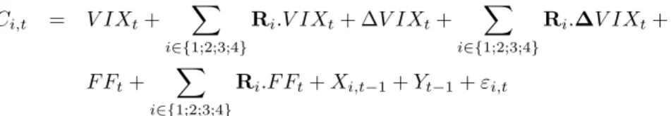
i ∈ {1; 2; 3; 4} where the low numbers denote fixed regimes and high numbers denote the floating regimes, using the Reinhart and Rogoff classification update as described above. We use the following specifications10:
Si,t = V IXt+ X i∈{1;2;3;4} Ri.V IXt+ ∆V IXt+ X i∈{1;2;3;4} Ri.∆V IXt+ F Ft+ X i∈{1;2;3;4} Ri.F Ft+ Xi,t−1+ Yt−1+ εi,t
10For a model that microfounds the use of the VIX and VIX growth rate in a regression
to explain credit creation see Bruno and Shin (2014). For another application see Miranda Agrippino and Rey (2013).
Ci,t = V IXt+ X i∈{1;2;3;4} Ri.V IXt+ ∆V IXt+ X i∈{1;2;3;4} Ri.∆V IXt+ F Ft+ X i∈{1;2;3;4} Ri.F Ft+ Xi,t−1+ Yt−1+ εi,t
Control variables are the lagged world GDP growth rate Yt−1and the lagged
country GDP Xi,t−1. The dummy interaction terms serve the purpose of
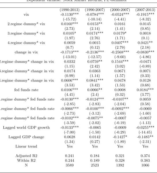
cap-turing the potential heterogeneous sensitivity of a given market to US monetary policy and to the Global Financial Cycle (proxied by the VIX) depending on the exchange rate regime. We run fixed effects estimators with clustered stan-dard errors by country. We have a large number of observations (between 1066 and 3982 depending on the specification). Tables 1 and 2 report the results of the regression for stock market returns (log difference of local stock market indices) and for credit growth (log difference in credit over GDP) respectively. For each regression we use monthly data over the 1990-2013 period and we split the sample in three subperiods: up to the crisis (1990 until 2007); the run up to the crisis (2000 until 2007) and the crisis period (2007-2013).
Table 1 shows the correlations between the domestic stock returns and the VIX and the Fed Funds rate. Stock returns are significantly negatively related to the VIX in all subperiods. The interaction terms between the Fed Funds Rate and the currency regime and the VIX (in log level and difference) and the currency regime denote the difference in the slopes of the benchmark case (pegged exchange rate regime, category 1 of Reinhart and Rogoff) and the slope of regimes 2, 3 and 4. Although some of the VIX exchange rate regime inter-actions are positive and significant, there is no pattern that could be linked to degree of exchange rate flexibility as there is great heterogeneity in the results across periods and across regimes. The only subperiods for which the flexible regime (4) is associated with a positive interaction term are the 2000-2007 and the 2007-2013 subperiods and during these periods the overall correlation be-tween the VIX and the stock returns is still negative. Similarly, whenever the interaction term between the exchange rate regime and the VIX is positive else-where (for example for regime 2 during 1990-2007), the overall effect remains negative. The change in VIX is also negatively related to the stock returns, with some positive interaction terms for the flexible exchange rates (regime 4) but also for relatively fixed rates (regime 2). The Fed Funds rate tends to be either positively associated with stock returns or insignificant. However, most interaction terms are negative and reverse the positive correlation to a negative one for most exchange rate regimes. Hence, more rigid regimes do not seem to be associated with a higher sensitivity of the stock market of country i to the Global Financial Cycle (or to the Fed Funds rate) in a systematic way.
[TABLE 1 ABOUT HERE]
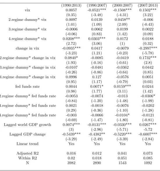
Domestic credit growth (Table 2) is significantly negatively related to the VIX in all subperiods except the crisis (2007-2013) where it is positively related
in levels but negatively related in difference. There is again no systematic re-lation between the VIX and the currency regime though the interaction term with the more flexible regime (4) and with the relatively fixed exchange rate regime (2) is again significant in some subperiods (without overturning the sign of the overall negative correlation). The correlation with the Fed Funds rate is positive and sometimes significant. Once again, there does not seem to be sys-tematic evidence that more rigid regimes are associated with a higher sensitivity of credit growth in country i to the US monetary policy or to the VIX.
It is very important to realize that the panel regressions of this section indi-cate only correlations and do not imply the existence of any form of causality. They are meant to illustrate cross sectional comovements with the Global Finan-cial Cycle across different exchange rate regimes. To summarize our results, we find that although there is some degree of heterogeneity in the sensitivities, no exchange rate regime seems to be systematically associated with a significantly lower sensitivity to the global financial cycle.
[TABLE 2 ABOUT HERE]
5
Global Financial cycle and US monetary
pol-icy
A natural next step in our investigation is to analyse the potential drivers of the global financial cycle. Given the importance of the US Dollar on interna-tional financial markets (see Portes and Rey (1998) Shin (2013)), one prime candidate is US monetary policy. In the domestic context financial market im-perfections have been shown to be important for the transmission of monetary policy: in the “credit channel” (Bernanke and Gertler (1995)), agency costs create a wedge between the costs of external finance and internal funds. This wedge depends on the net worth of firms, banks, households or on value at risk constraints (see Adrian and Shin (2014), Bruno and Shin (2014), Borio and Zhu (2011)) and therefore inter alia on monetary policy. As Rey (2014) points out, the international role of the dollar as a funding currency and as an in-vestment currency suggests that US monetary policy by affecting the net worth of investors, intermediaries and firms worldwide may transmit US monetary conditions across borders and jurisdictions. Hence, the existence of an ”inter-national credit channel” that propagates the global financial cycle. In order to investigate empirically the nature of such a transmission mechanism, we need to evaluate the combined responses of a set of economic and financial variables such as mortgage spreads, which are a measure of the external finance premium to US monetary policy surprises.
As underlined by Stock and Watson (2008, 2012), the identification problem in structural VAR analysis is how to go from the moving-average representation
in terms of the innovations to the impulse response function with respect to a unit increase in the structural shock of interest, which is here the US mone-tary policy shock. Traditionally, imposing economic restrictions such as timing restrictions (some variables move within the month, others are slower mov-ing) have permitted identification of the coefficients (see Bernanke and Gertler (1994), Christiano,et al. (1996))11. When one tries to identify the international
credit channel of monetary policy, movements in asset prices and spreads are key, as they are related to the external finance premium or the operation of value at risk constraints. Hence, it is of the utmost importance to use an iden-tification strategy which allows for immediate response in asset prices, as there is certainly no delay in those market reactions. We follow Gertler and Karadi (2014) whose approach brings together vector autoregression (VAR) analysis and high frequency identification (HFI) of monetary policy shocks and use the Gurkaynak et al.(2005) surprise measures as external instruments in our VAR12.
These are very clever instruments as they measure surprises as changes in Fed funds futures in tight windows around monetary policy announcement times. As Fed funds future prices aggregate all available information about expected monetary policy rates prior to FOMC meetings, any change in their prices at the time of the meeting is very likely reflecting only a monetary policy surprise. It is indeed unlikely that any other event dominates fluctuations in the prices of Fed funds futures in a 30 minute or 15 minute window around the announce-ment. Their approach addresses the simultaneity issue of monetary policy shifts, which influence and at the same time respond to financial variables. Following Gertler and Karadi (2014), we use these surprises to instrument the one year US interest rate in our VAR. The advantage of instrumenting the one year rate (as opposed to the Fed Funds rate) is that the effect of forward guidance can be taken into account in the estimates. This is of course particularly important in a period where the Fed Funds rate has hit the zero lower bound.
5.1
Methodology
Our vector autoregression contains both economic and financial variables. To identify monetary surprises we use external instruments following Gertler and Karadi (2014) who use a variation of the methodology developed by Stock and Watson (2012) and Mertens and Ravn (2013) . Let
AIt= m
X
k=1
CkYt−k+ εt
11As is well known, Romer and Romer (1989, 2004) introduce what has been called the
”narrative approach”, that is to say use information from outside the VAR to construct exogenous components of specific shocks.
12For another recent study where external instruments are used to identify the structural
be our general structural form. The reduced form representation can be then written as follows: It= m X k=1 DkYt−k+ ut
where the reduced form shock ut is a function of the structural shocks:
ut= P εt, where Dk = A−1Ck and P = A−1.
We define Σ the variance-covariance matrix of the reduced form model. For Σ, we have: Σ = E[utu 0 t] = E[P P 0] We assume im
t ∈ It, to be the monetary policy indicator, and in particular
the US government bond rate with one-year maturity as analytically discussed in the previous section. The exogenous variation of the policy indicator stems from the policy shock εm
t .
Finally, p stands for the column in P corresponding to the impact of the policy shock εm
t on each element of the vector of reduced form residuals ut. For
the impulse responses of our economic and financial variables to a policy shock we run: It= m X k=1 DkYt−k+ pεmt
As discussed in the previous section, standard timing restrictions are prob-lematic in the presence of financial variables. For this reason, we follow the identification strategy of Gertler and Karadi (2014) and employ their external instruments. In order for the vector of instrumental variables Zt to be a valid
set of instruments for the monetary policy shock εm
t we need: E[ztεm 0 t = φ] and E[ztεd 0 t = 0] where εd
t stands for any structural shock but the monetary policy shock.
In order to compute the estimates of vector p, as a first step we need to compute the estimates of the reduced form residuals vector ut from the least
squares regression of the reduced form representation. We denote ud
tthe reduced
form residual from the equation for variable d which is different from the policy indicator and umt the reduced form residual from the equation for the policy
indicator. Additionally, assume that pd ∈ p is the response of ud
t to a unit
increase in the policy shock εmt . From the two stage least squares regression of udt on umt and using the vector of instrumental variables Zt, one can compute
an estimate of the ratio pd/pm .
In particular, the variation in the reduced form residual for the policy indi-cator due to the structural policy shock is first isolated by regressing um
t on the
vector of instruments yielding cum
t . As the variation in cumt is only due to εmt ,
a second stage regression of udt on cumt provides a consistent estimate of pd/pm.
The estimated reduced form variance-covariance matrix is then used to obtain an estimate of pmusing the second stage regression, allowing to identify pd 13.
5.2
Results
We analyse the effect of US monetary policy shocks on the global financial cycle (through the VIX) as well as on the US external finance premium. We then study the effect of US monetary policy shocks on a mostly floating exchange rate economy (the UK). According to the traditional Mundell Fleming model and the trilemma, the UK should be insulated from US monetary policy spillovers by movements in the dollar pound rate and should be able to set its own monetary and financial conditions. Our empirical strategy allows us to test whether the ”international credit channel” is potent enough to put this classic idea into question14.
US monetary policy and the Global Financial Cycle
We consider a monthly VAR on data ranging between 1979 and 2012, that includes real economy variables such as US industrial production (seasonally adjusted) and the US CPI as well as variables capturing the external finance premium (US mortgage spread and US corporate bond spread). We also include the VIX as a proxy for the Global Financial Cycle, tightly correlated with global leverage, gross cross border flows and the global component in risky asset prices. As discussed above, we use external instruments based on Fed Funds rate futures surprises to identify the monetary policy shocks15. We replicate the results of Gertler and Karadi (2014) and find (see figure 6) , for a 20 bp shock to the US one year rate a strong reaction of the mortgage spread (peak about 8 bp) and of the US corporate spread (about 6 bp). Extending our analysis to global variables, we also find that a 20 bp shock in the one year rate leads to a 5 bp shock to the VIX (logged, a standard deviation in the log VIX is 15.2 bp). We read these Impulse Response Functions as supporting the importance of the credit channel of monetary policy both domestically and internationally. When the Federal Reserve tightens, the VIX goes up and global asset prices go down. In Miranda Agrippino and Rey (2012), we use a large Bayesian VAR with 22 variables in
13For more details see Gertler an Karadi (2014) and Mertens and Ravn (2013).
14For a detailed discussion of the international credit channel and of the relevant empirical
evidence see Rey (2014).
15We are very grateful to Mark Gertler and Peter Karadi for having shared their data and
quarterly data to study the effect of US monetary policy on the global financial cycle. We use the narrative approach of Romer and Romer (2004) to identify the monetary policy shocks. Our results also support the existence of a significant effect of a Fed tightening on credit creation, capital flows, leverage of global banks and external finance premia and global asset prices. It is comforting that two very different methodologies (a small VAR with external instruments and a large Bayesian VAR with different external instruments) give very consistent results.
[FIGURE 6 ABOUT HERE]
Figure 6: Response of the VIX to a 20bp increase in the US one year rate. Instruments from Gertler and Karadi(2014)
US monetary policy spillovers into a floating exchange rate country
The ubiquity of the global financial cycle and our previous panel results seem to indicate that even flexible exchange rate regime countries are not insulated from global factors, yet, it is worth exploring this important question in more detail. We estimate directly the effect of US monetary policy shocks on activity,
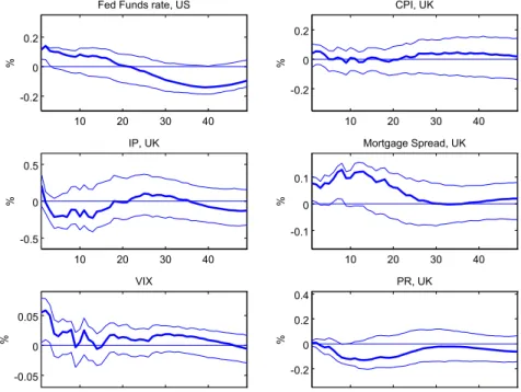
inflation and the external finance premium for the United Kingdom, an advanced economy that embraced inflation targeting. We rely on the same estimation strategy as above. The variables in the UK VAR are industrial production, the CPI, the domestic policy rate, the mortgage spread (most widely available series with a long time span across countries) and the VIX. Using the mortgage spread has an additional advantage: the real estate market is central for financial stability and has been shown to be very important in boom bust cycles around the world. In the domestic UK context, a 17 bp increase in the US one year rate leads to a 8 bp increase in the mortgage spread within half a year. In the UK, a US tightening also has a significant effect on mortgage spreads. It peaks at about 12 bp around 9 months after the tightening. This is of the same order of magnitude as in the US. Rey (2014) covers an extended set of inflation targeters and finds similar results, though with some degree of heterogeneity. It seems that financial conditions as measured by mortgage spreads respond to US monetary policy shocks rapidly in the UK. Whether one considers this as a very potent transmission channel of monetary policy has to depend on whether one thinks that channel is an important one within US borders. If one does, one is left with the conclusion that the international credit channel cannot be neglected. 10 20 30 40 -0.2 0 0.2 %
Fed Funds rate, US
10 20 30 40 -0.2 0 0.2 % CPI, UK 10 20 30 40 -0.5 0 0.5 % IP, UK 10 20 30 40 -0.1 0 0.1 % Mortgage Spread, UK 10 20 30 40 -0.05 0 0.05 % VIX 10 20 30 40 -0.2 0 0.2 0.4 % PR, UK
Figure 7: Response of the UK (% points) to a 20bp increase in the US one year rate(HF instruments of Gertler and Karadi(2014))
[FIGURE 7 ABOUT HERE]
6
Conclusions
Economists and policy makers have emphasized allocative efficiency and risk sharing as the main sources of potential gains from financial integration follow-ing the insights of the textbook neoclassical growth model. But the quantitative evaluation of these models shows that these gains are not very big. Together with the relatively non conclusive large empirical literature on financial integra-tion, this leads us to believe that large welfare gains from financial integration are hard to find. This is particularly striking given the scale of cross border financial flows which have increased massively. Large gross cross border flows are moving in tandem across countries regardless of the exchange rate regime, they tend to rise in periods of low volatility and risk aversion and decrease in periods of high volatility and risk aversion, as measured by the VIX. Risky asset prices around the world are also largely driven by one global component tightly correlated to the VIX. Leverage and credit across countries show significant de-grees of co-movements (and are negatively correlated with the VIX). There is a global financial cycle. We find that the correlations of stock prices and credit growth with the global financial cycle (proxied by the VIX) do not seem to vary systematically with the exchange rate regime. Using a VAR methodolody with external instruments, we also show that US monetary policy has an effect on the VIX (a US tightening increases the VIX). Importantly we find that US monetary policy has also an effect the United Kingdom’s external finance pre-mium (measured by the mortgage spread), even though the UK has a floating exchange rate regime. This seems to indicate that the insulating properties of floating regimes may have been overestimated. It would be desirable to estimate the effect of a Fed tightening on other measures of financial conditions (corpo-rate spreads, effect on the term premium) and on a broader set of countries. It would also be important to disentangle the two main channels through which the dependence of UK monetary conditions (evidenced by the mortgage spread reaction) on the policy stance of the United States could take place. The first one is the ”fear of floating” (Calvo and Reinhart (2002)) whereby Central Banks threatened by large capital flows could try to reduce the interest rate differential with the Federal Reserve. The second one is the international credit channel whereby even if the domestic policy rate remains unaltered domestic financial conditions are affected by the change in monetary policy of the Federal Reserve via the role of the dollar as an international currency. Future research will no doubt shed further light on these issues16.
References
[1] Adrian, Tobias and Shin, Hyun Song. Pro-cyclical leverage and value-at-risk. Review of Financial Studies, 27:373–403, 2014.
[2] Bernanke, Ben and Gertler, Mark. Inside the black box: The credit channel of monetary policy transmission. Journal of Economic Perspectives, 9:27– 48, 1995.
[3] Borio, Claudio and Zhu, Haibin. Capital regulation, risk-taking and mon-etary policy: a missing link in the transmission mechanism? forthcoming in Journal of Financial Stability, 2011.
[4] Bruno, Valentina and Shin, Hyun Song. Cross-border banking and global liquidity. Review of Economic Studies, forthcoming, 2014.
[5] Calvo, Guillermo A. and Reinhart, Carmen M. Fear of floating. Quaterly journal of economics, (2):379–408, 2002.
[6] Christiano, Lawrence J., Eichenbaum, Martin, and Evans, Charles. The effects of monetary policy shocks: Evidence from the flow of funds. The Review of Economics and Statistics, 78:16–34, 1996.
[7] Coeurdacier, Nicolas and Rey, H´el`ene. Home bias in open economy financial macroeconomics. Journal of Economic Literature, 51(1):63–115, 2012. [8] Coeurdacier, Nicolas, Rey, H´el`ene, and Winant, Pablo. Financial
integra-tion and growth in a risky world. London Business School and SciencesPo manuscript, 2013.
[9] Danielsson, Jon, Song Shin, Hyun, and Zigrand, Jean-Pierre. Balance sheet capacity and endogenous risk. FMG discussion paper series, 665. Finan-cial Markets Group, London School of Economics and Political Science, London, UK, 2011.
[10] Drehmann, Mathias, Borio, Claudio, and Tsatsaronis, Kostas. Character-ising the financial cycle: don’t lose sight of the medium term! BIS Working Papers, no 380, 2012.
[11] Forbes, Kristin and Warnock, Francis E. Capital flow waves: Surges, stops, flight and retrenchment. Journal of International Economics, 88:235–251, 2012.
[12] Gertler, Mark and Karadi, Peter. Monetary policy surprises, credit costs, and economic activity. American Economic Journal: Macroeconomics, forthcoming, 2014.
[13] Goldberg, Linda. Banking globalization, transmission, and monetary pol-icy autonomy. Sveriges Riksbank Economic Review, Special Issue:161–193, 2013.
[14] Gourinchas, Pierre-Olivier, Govillot, Nicolas, and Rey, H´el`ene. Exorbitant privilege and exorbitant duty. London Business School manuscript, 2010. [15] Gourinchas, Pierre-Olivier and Jeanne, Olivier. The elusive gains from
international financial integration. Review of Economic Studies, 73:715741, 2006.
[16] Gourinchas, Pierre-Olivier and Rey, H´el`ene. Chapter for the Handbook of International Economics in Gopinath, Helpman and Rogoff eds., chapter External Adjustment, Global Imbalances and Valuation Effects. 2014. [17] Gourinchas, Pierre-Olivier, Rey, Helene, and Truempler, Kai. The
finan-cial crisis and the geography of wealth transfers. Journal of International Economics, 88.
[18] Gurkaynak, Brian, Refet S.and Sack and Swanson, Eric T. Do actions speak louder than words? the response of asset prices to monetary policy actions and statements. International Journal of Central Banking, 1:55–93, 2005.
[19] Ilzetzki, Ethan O. and Reinhart, Carmen. Exchange rate arrangements entering the 21st century: Which anchor will hold? Working paper, 2009. [20] Jeanne, Olivier, Subramanian, Arvind, and Williamson, John. Who needs
to open the capital account? Peterson Institute for International Eco-nomics, 2012.
[21] Keynes, John Maynard. The Economic Consequences of the Peace. Har-court, Brace, and Howe, Inc. Library of Economics and Liberty, New York, 1920.
[22] Klein, Michael and Shambaugh, Jay. Rounding the corners of the policy trilemma: Sources of monetary policy autonomy. NBER Working Papers 19461, National Bureau of Economic Research, Inc., 2013.
[23] Lane, Philip R. and Milesi-Ferretti, Gian Maria. A global perspective on external positions. In Clarida, Richard, editor, G-7 Current Account Im-balances: Sustainability and Adjustment, 2007.
[24] Lewis, Karen. Trying to explain home bias in equities and consumption. Journal of Economic Literature, 37:571 – 608, 1999.
[25] Lewis, Karen. Why do stocks and consumption suggest such different gains from international risk-sharing? Journal of International Economics, 52:1 –35, 2000.
[26] Lewis, Karen and Liu, Edith. Evaluating international consumption risk sharing gains: An asset return view. Journal of Monetary Economics, forthcoming, 2014.
[27] Mertens, Karel and Ravn, Morten O. The dynamic effects of personal and corporate income tax changes in the united states. American Economic Review, 103:1212–1247, 2013.
[28] Miranda Agrippino, Silvia and Rey, H´el`ene. World asset markets and global liquidity. presented at the Frankfurt ECB BIS Conference, London Business School, mimeo, 2012.
[29] Obstfeld, Maurice. International finance and growth in developing coun-tries: what have we learned? IMF staff papers vol 56, 2009.
[30] Obstfeld, Maurice. Trilemmas and tradeoffs: Living with financial global-ization. University of California, Berkeley, Working paper, 2014.
[31] Obstfeld, Maurice, Shambaugh, Jay, and Taylor, Alan. The trilemma in history: Tradeoffs among exchange rates, monetary policies, and capital mobility. Review of Economics and Statistics, 87:423–438, 2005.
[32] Obstfeld, Maurice and Taylor, Alan. Global Capital Markets: Integration, Crisis, and Growth. Cambridge University Press, UK, 2004.
[33] Portes, Richard and Rey, H´el`ene. The emergence of the euro as an inter-national currency. Economic Policy, pages 305–343, April 1998.
[34] Reinhart, Carmen and Rogoff, Kenneth. The modern history of exchange rate arrangements: A reinterpretation. Quarterly Journal of Economics, 119:1–48, 2004.
[35] Rey, H´el`ene. Dilemma not trilemma: The global financial cycle and mon-etary policy independence. In Jackson Hole Economic Symposium, 2013. [36] Rey, H´el`ene. The international credit channel and monetary policy
auton-omy. IMF Mundell Fleming Lecture, November 2014.
[37] Romer, Christina D. and H., Romer David. Does Monetary Policy Matter? A New Test in the Spirit of Friedman and Schwartz. NBER Macroeco-nomics Annual in Blanchard and Fischer eds., MIT Press, 1989.
[38] Romer, Christina D. and H., Romer David. A new measure of monetary shocks: Derivation and implications. The American Economic Review, 94:1055–1084, 2004.
[39] Shin, Hyun Song. Global banking glut and loan risk premium. Mundell-Fleming Lecture, IMF Economic Review, 60:155–192, 2012.
[40] Stock, James H. and Watson, Mark W. Econometrics course, NBER sum-mer institute. 2008.
[41] Stock, James H. and Watson, Mark W. Disentangling the channels of the 2007-09 recession. Brookings Papers on Economic Activity, 44:81–135, 2012.
[42] Van Wincoop, Eric. Welfare gains from international risksharing. Journal of Monetary Economics, 34:175–200, 1994.
[43] Van Wincoop, Eric. How big are potential gains from international riskshar-ing? Journal of International Economics, 47:109–135, 1999.
Table 1: Panel Regression Results, Sample Period: 1990-2013
Dependent variable: Stock Market Returns, FE estimator
(1990:2013) (1990:2007) (2000:2007) (2007:2013) vix -0.1130*** -0.0784*** -0.0524*** -0.1915***
(-15.72) (-10.14) (-4.41) (-8.32) 2.regime dummy* vix 0.0160*** 0.0153** 0.0161 0.0145
(2.73) (2.14) (1.41) (0.85)
3.regime dummy* vix 0.0105* 0.0174*** 0.0179* 0.0018
(1.97) (2.76) (1.71) (0.1)
4.regime dummy* vix 0.0059 0.0015 0.0407*** 0.0421**
(0.7) (0.12) (2.79) (2.18)
change in vix -0.1713*** -0.2136*** -0.2568*** -0.0830*** (-13.01) (-12.57) (-9.60) (-4.86) 2.regime dummy* change in vix 0.0332 0.0759** 0.1544*** -0.0471
(1.15) (2.42) (3.02) (-0.89)
3.regime dummy* change in vix 0.0174 0.0363 0.0671 0.0071
(0.99) (1.14) (1.57) (0.33)
4.regime dummy* change in vix 0.0606*** 0.0841*** 0.0478 0.0128
(3.53) (3.42) (1.53) (0.68)
fed funds rate 0.0106*** 0.0066** 0.0008 0.0184***
(4.45) (2.4) (0.32) (3.77)
2.regime dummy* fed funds rate -0.0130*** -0.0124*** -0.0107** 0.0059
(-2.85) (-2.83) (-2.04) (0.58)
3.regime dummy* fed funds rate -0.0066*** -0.0100*** -0.0092*** -0.0069 (-2.73) (-3.12) (-2.69) (-1.60) 4.regime dummy* fed funds rate -0.0102*** -0.0075** -0.0007 -0.0057 (-3.59) (-2.02) (-0.19) (-1.13) Lagged world GDP growth -0.0133*** -0.0065 -0.0009 -0.0255***
(-7.00) (-1.50) (-0.29) (-14.45)
Lagged GDP change 0.0628 0.0142 -0.1427* -0.1485**
(1.34) (0.27) (-1.89) (-2.31)
Linear trend Yes Yes Yes Yes
Adjusted R2 0.241 0.184 0.321 0.374
Within R2 0.244 0.189 0.328 0.383
N 3589 2523 1392 1066
Fixed effect estimator, standard errors adjusted for clustering on country, t-stat in parentheses. All specifications include the control variables and a linear trend
Table 2: Panel Regression Results, Sample Period: 1990-2013
Dependent variable: Domestic Credit to GDP Market Returns, FE estimator (1990:2013) (1990:2007) (2000:2007) (2007:2013)
vix 0.0057 -0.0521*** -0.1508*** 0.1502***
(0.35) (-3.48) (-4.31) (3.22)
2.regime dummy* vix 0.0097 0.0139 0.0458** -0.006
(1.01) (1.09) (2.09) (-0.43)
3.regime dummy* vix -0.0006 0.0062 0.0199 0.0022
(-0.06) (0.83) (1.42) (0.09)
4.regime dummy* vix 0.0208*** 0.0303*** 0.0172 0.0188
(2.72) (3.06) (1) (0.32)
change in vix -0.0935*** 0.0417 -0.0079 -0.2997***
(-3.23) (1.21) (-0.23) (-5.78)
2.regime dummy* change in vix 0.0840* -0.0085 -0.0419 0.1732***
(1.93) (-0.16) (-0.61) (2.8)
3.regime dummy* change in vix -0.0107 -0.0481 -0.0362 0.0442
(-0.26) (-0.86) (-0.64) (0.85)
4.regime dummy* change in vix 0.0996 0.127 -0.0576 0.0051
(0.95) (1.17) (-0.79) (0.03)
fed funds rate 0.0044 0.0071* 0.0159*** 0.0244
(0.98) (1.77) (3.11) (1.42)
2.regime dummy* fed funds rate -0.0053 -0.0074 -0.013 -0.0306* (-0.84) (-1.20) (-1.48) (-1.99) 3.regime dummy* fed funds rate 0.0021 -0.0018 -0.0076 -0.0202
(0.29) (-0.36) (-1.10) (-1.28)
4.regime dummy* fed funds rate -0.003 -0.0066 -0.0104* -0.0121 (-0.69) (-1.47) (-1.80) (-0.81) Lagged world GDP growth 0.0074*** -0.0131*** -0.0330*** 0.0267***
(3) (-2.96) (-5.71) -5.72
Lagged GDP change -0.5439*** -0.4382** -0.5220*** -0.6007*** (-3.29) (-2.49) (-3.39) (-2.84)
Linear trend Yes Yes Yes Yes
Adjusted R2 0.016 0.012 0.041 0.073
Within R2 0.02 0.018 0.051 0.085
N 3982 2890 1543 1092
Fixed effect estimator, standard errors adjusted for clustering on country, t-stat in parentheses. All specifications include the control variables and a linear trend
Data Appendix A
List of Countries Included
North Latin Central and Western Emerging Asia Africa
America America Eastern Europe Europe Asia
Canada Argentina Belarus Austria China Australia South Africa
US Bolivia Bulgaria Belgium Indonesia Japan
Brazil Croatia Cyprus Malaysia Korea
Chile Czech Republic Denmark Thailand New Zealand
Colombia Hungary Finland
Costa Rica Latvia France
Ecuador Lithuania Germany
Mexico Poland Greece
Romania Iceland
Russian Fed. Ireland
Serbia Italy
Slovak Republic Luxembourg
Slovenia Malta Turkey Netherlands Norway Portugal Spain Sweden Switzerland UK
Data Appendix B
Global Factor: common factor extracted from a collection of 858 asset price series spread over Asia Pacific, Australia, Europe, Latin America, North Amer-ica, Commodity and Corporate samples. For details on extraction and original asset prices dataset composition please refer to Miranda Agrippino and Rey (2012).
Banking Sector Leverage: constructed as the ratio between Claims on Private Sector and Transferable plus Other Deposits included in Broad Money of Depository Corporations excluding Central Banks. Data are in national cur-rencies from the Other Depository Corporations Survey; Monetary Statistics, International Financial Statistics database. Classification of deposits within the former Deposit Money Banks Survey corresponds to Demand, Time, Savings and Foreign Currency Deposits.
Exchange rate regime data from Carmen Reinhart’s website: We use the Exchange Rate Regime Reinhart and Rogoff Classification and construct are dummies using the monthly coarse classification. For the purposes of the panel regression analysis as well as for the construction of the correlation heatmaps we exclude categories 5 and 6 as the number of occurrences is very small for these regimes. The exact classification criteria are presented in the exhibit below:
Regime Classification Codes 1 No separate legal tender
1 Pre announced peg or currency board arrangement
1 Pre announced horizontal band that is narrower than or equal to +/-2% 1 De facto peg
2 Pre announced crawling peg
2 Pre announced crawling band that is narrower than or equal to +/-2% 2 De factor crawling peg
2 De facto crawling band that is narrower than or equal to +/-2% 3 Pre announced crawling band that is wider than or equal to +/-2% 3 De facto crawling band that is narrower than or equal to +/-5%
3 Moving band that is narrower than or equal to +/-2% (i.e., allows for both appreciation and depreciation over time)
3 Managed floating 4 Freely floating 5 Freely falling
6 Dual market in which parallel market data is missing.
For the panel regression we map the regime to the constructed dummy vari-able which allow us to use a dynamic indicator for each country. When building the correlation heatmap we order the currencies according to their overall
”rigid-ity”, which we calculate by averaging the regime number of a country’ currency over the sample period.
Domestic Credit: constructed as the sum of domestic claims of Depos-itory Corporations excluding Central Banks. Domestic claims are defined as Claims on Private Sector, Public Non-Financial Corporations, Other Financial Corporations and Net Claims on Central or General Government (Claims less Deposits); Other Depository Corporation Survey and Deposit Money Banks Survey; Monetary Statistics; IFS. Original data in national currencies.
Direct Cross-Border Credit: measured as difference in claims on all sectors or non-bank sector of a given country of all BIS reporting countries in all currencies; Locational Statistics Database; International Bank Positions by Residence; BIS; Tables 7A and 7B.
Nominal GDP Data in USD: original data in national currencies from National Statistical Offices; Haver Analytics conversion using spot end of period FX rates.
VIX: end of period readings; Chicago Board Option Exchange (CBOE). Stock Market Indices: end of period close quotes; Haver Analytics and Global Financial Data.
House Price Indices: OECD, BIS. Data on Capital flows:
Source of flow data: quarterly gross capital inflows and outflows from the In-ternational Monetary Fund’s InIn-ternational Financial Statistics (accessed through IMF website in March 2013) for: Portfolio Equity Inflows, Outflows and Net Flows constructed as Outflows-Inflows (Assets-Liabilities) FDI Inflows, Outflows and Net Flows Portfolio Debt Inflows, Outflows and Net Flows, and Other In-vestment Inflows, Outflows and Net Flows Data transformations: Flows are reported in millions of U.S. dollars
IFS does not differentiate between true zeros and not availables; most of the times we treat these values as errors and omissions, unless they evidently represent zero flows. Mapping of the flows from BPM5 (until 2004 Q4) to BP6 (2005 Q1 onwards) in accordance to the guidelines of the 6th edition of the Balance of Payments and International Investment Position Manual of IMF – Reconciliation for quarters 2005 Q1 - 2008 Q4 for which there is data overlap. Construction of Net Flows only when data on Inflows and Outflows are available
World GDP Growth (Quarterly): International Monetary Fund’s Interna-tional Financial Statistics (accessed through IMF website in March 2013).
US GDP: Real Gross Domestic Product (Billions of Chained 2005 Dollars); Bureau of Economic
VAR Analysis
US Data
We thank Mark Gertler and Peter Karadi for kindly providing us with the data used in the US monthly VAR. We compliment their analysis by adding the VIX series (logged) to the VAR.
UK Data
For the data used in the UK VAR spanning a period between 1995 and 2014, we additionally employ: -Monthly CPI data and monthly industrial production data (seasonally adjusted) from the IMF (IFS database). -A constructed mort-gage spread series using monthly data from the Bank of England. The mortmort-gage spread is calculated as the difference of the Bank Rate Tracker (series bv24) (extended further back with the Standard Variable Rate) from the 3M LIBOR. -The UK policy rate calculated as a monthly average of the Official Bank rate from the Bank of England.