Consumption Structure, Welfare Goods and Retirement Income: Linking the Ageing Puzzles

CONSUMPTION STRUCTURE, WELFARE GOODS AND RETIREMENT INCOME: LINKING THE AGEING PUZZLES

Najat El-Mekkaoui de Freitas

(Université Paris-Dauphine, Laboratoire d’Économie)

and

Joaquim Oliveira Martins

(OECD and Université Paris-Dauphine, Laboratoire d’Économie)

Abstract

While the empirical evidence tends to support some predictions of the life-cycle theory, a number of puzzles remain: an ageing-consumption, an ageing-saving, a saving-capitalisation and a saving-longevity puzzles have been put forward in the literature. This paper analyses the links between these puzzles and develops a model relating usual life-cycle variables, social transfers (public health care expenditures and the generosity of pension systems) to the level of savings. A reduced-form model using a panel of 18 OECD countries is tested, confirming the proposed explanations for the puzzles, together with other factors such as public deficits (Ricardian equivalence) and the population structure. We found that the relative generosity of welfare systems have a significant negative impact on household saving rate. It can also explain why the increase in longevity does not have had in general a positive impact on the household saving ratio.

JEL Classification: C68, D91, G10, J11, J26

Key words: Ageing, consumption, longevity, pensions, saving

Revised version May 2009

(*) El-Mekkaoui de Freitas: Laboratoire d‟Économie de Dauphine (LEDa), Université Paris-Dauphine, 75116 Paris, Email: [email protected], Oliveira: OECD, 2 Rue André Pascal, 75775 Paris Cedex 16, Email: [email protected]. The authors would like to thank Philippe Bernard, Henri Sterdyniak, Carole Bonnet and an anonymous referee for comments on an earlier version of this paper. We also would like to thank the participants at the Banca d‟Italia Workshop on Public Finance, 2009, in particular Johannes Clemens. This work was supported by the Chaire Dauphine-Ensae Groupama and is gratefully acknowledged by the authors. The views expressed are those of the authors and do not reflect those of the OECD or its Member countries.

1. Motivation

The life cycle model is the main framework used in economics to understand the relations between ageing, consumption and saving behaviour. While main predictions of the life cycle theory tend to be supported by empirical evidence, a number of puzzles remain. The literature has put forward four main types of puzzles: an ageing-consumption puzzle, an ageing-saving puzzle, a saving-capitalization puzzle and a saving-longevity puzzle.

The first puzzle concerns the tendency for consumption to decrease in old age. This stylised fact observed in all OECD countries, seems to contradict the idea that households save in order to maintain their consumption level after retirement. Second, significant levels of savings are observed at old age. Another puzzling fact is that countries with generous PAYG system and health care system (welfare goods) have the highest private saving rate. In contrast, in countries where pension funds are well developed, the private saving rate is much lower. Finally, an increase in longevity by increasing the duration of the retirement period could be expected to increase the saving ratio.1 However, when empirically tested, the sign of longevity variables in traditional saving equations is often negative.

An extensive literature has put forward potential explanations for each of the puzzles, but, to our knowledge, there has been no attempt to bring all of them together in an integrated view. We argue in this paper that the four puzzles are interlinked. As discussed below, the interaction between consumption and provision of welfare goods and the level of retirement income can indeed explain a large part of these phenomena. In order to highlight the role of these determinants and their links, it is instrumental to compare household saving behaviour, health and retirement systems of two country groupings: those with PAYG systems and those with fully-funded systems. Other traditional determinants of savings have also to be brought into the picture, in particular the role of Ricardian compensation between private and public savings, as well as income.

The paper begins with a review of empirical facts on consumption, savings and pensions that generate the puzzles referred above. In order to guide our intuition concerning the relationships among the key variables, we develop in section 3 a two-period life cycle model where we consider the optimal welfare consumption, welfare transfers, the generosity of pension systems and longevity. In section 4, we get back to the facts and present some possible explanations of the ageing puzzles. In section 5, we then present econometric panel estimates that combine both the relationships derived from the theoretical framework, other additional effects and controls often used in the empirical literature. A final section concludes.

2. The Ageing puzzles: Consumption, Saving and Longevity

The most useful framework to study the link between ageing, consumption and saving is the life cycle model (Modigliani and Brumberg, 1954; Friedman, 1957). In its simplest version, individuals live two periods. In the first period each person earns a wage from his or her labour supply and in the

1. This of course only holds when the age of retirement is fixed and not linked to longevity, which is still the case in most social security systems in OECD countries.

second period the person is retired. Individuals save from their wage income to provide for second period consumption with a constant rate of interest (i.e., the rate of interest does not vary with the level of saving). The main result obtained from this framework is that the consumption is smoothed: the individuals will save in order to transfer purchasing power to the period of the retirement.

But some empirical facts on consumption, pension and saving do not fit well with the basic life-cycle model. The first puzzle concerns the link between ageing and consumption. A large body of literature has found that consumption falls significantly at retirement, a fact somewhat in contradiction with life-cycle consumption smoothing. This applies over a number of countries (e.g. US, UK and Italy), across different time periods and across different measures of spending. This stylized fact is displayed in Figure 1, relating levels of household consumption by age for the US and several European countries.

[Figure 1. The Ageing-Consumption puzzle]

While household survey data suggest that total consumption displays a hump-shaped profile across age-groups,2 this is not equivalent to say that the consumption profile is hump-shaped over the life cycle mainly due to the existence of cohort and time effects.3 Nonetheless, they would suggest that the pure consumption-smoothing hypothesis is only partly supported by the micro data.4

Several explanations of this puzzle have been put forward. Allowing for uncertainty, Banks, Blundell and Tanner (1998) suggest that unanticipated shocks that occur around the time of retirement could explain the fall in spending within the context of the life-cycle model. Bernheim, Skinner and Weinberg (2001) suggested that workers do not adequately foresee the decline in income associated with the retirement. Hurd and Rohwedder (2003) argue that the drop in spending can still be explained by an extended version of the life-cycle model, where certain work-related consumption expenditures stop at retirement and market-purchased goods & services are substituted by household home production. The latter could be the case of long-term care services, which often are provided informally within families. However, in a more recent paper, Hurd and Rohwedder (2006) argue, like others, that the reduction in consumption cannot be explained by the simple one-good life cycle model with forward-looking consumers. Many factors such as leisure or poor health could also explain the decline in spending. Along these lines, Smith (2007) argues that retirement is involuntary, largely reflecting ill health status and redundancy, and likely to be associated with a negative wealth shock.

The second puzzle is closely related to the previous one, although is not equivalent. With a certain stability of retirement incomes and a decline in consumption, positive saving at old ages can be

2. To be precise, the consumption profile is hump-shaped across households headed by individuals belonging to

different age groups.

3. Due to the lack of data, it will be assumed that the snapshot picture of total consumption per household by age-groups approximates the life-time consumption profile of a cohort (e.g. static ageing as opposed to

dynamic ageing). This approach takes an agnostic view on how a combination of various household

characteristics in conjunction with institutional factors in each country affects the life-cycle consumption pattern. Fernandez-Villaverde and Krueger (2002) suggest that the bias induced by the use of age-groups instead of cohorts may not be very large for the estimation of the hump-shaped consumption profiles.

4. Attanasio (1999) provides an overview of competing theories of consumption behaviour over the life cycle. Note that when the income profile is more hump-shaped than consumption, the above observed age-consumption patterns are still compatible with some age-consumption smoothing over the life cycle.

observed (see Börsch-Supan et al., 2000; Börsch-Supan and Winter, 2001). However, it is puzzling that individuals cannot anticipate this fact and continue to save at old age, in particular in countries with generous welfare goods (high pension replacement rates and health care coverage).

Bloom et al. (2003) and Sheshinski (2004) suggest that higher life expectancy may increase the need for additional precautionary savings, despite the effect of improved health care on the length of desired working life. Moore and Mitchell (1998) also conclude that Americans are not preparing adequately for retirement as a couple would need to save 20% of annual earnings between 1992 and the time of retirement (at 62) to have a replacement rate of 61%. A single woman would need to save around 32% of her income to have a replacement ratio of 54% at age of 62. They conclude, despite seemingly large accumulations of total retirement wealth, the majority of older households will not be able to maintain current levels of consumption into retirement without additional saving. Bernheim et al. (2001) argue their results are difficult to reconcile with the life-cycle model and that they are more likely to be the result of household behaviour not governed by rational, farsighted optimization. Khitatrakun and Scholz (2004) note that tax incentives, like IRAs and 401(k) are not needed and may lead to excess savings. Finally, a largely evoked, but not well documented, reason for saving at older ages is the existence of bequest motives.

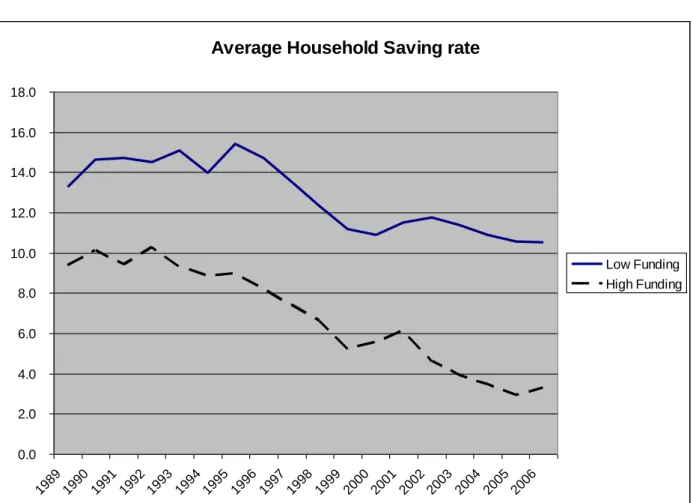
The third puzzle arises from the fact that countries with fully funded systems have the lowest private saving rates. In principle, the introduction of a fully-funded pension system should induce a decline in the replacement rate of PAYG systems and, according to the life-cycle model, increase aggregate savings. Figure 2 shows that while saving rates have been decreasing steadily in all countries, the countries with PAYG systems have persistently displayed higher household saving rates and the gap has widened over time.

[Figure 2. The Saving-Capitalisation puzzle]

In a seminal paper, Feldstein (1974) highlighted a negative link between PAYG pension systems and household savings. But, subsequent empirical tests on the impact of pension systems on household saving have produced mixed results (e.g. Edwards, 1996; Callen-Thimann, 1997; Corsetti, Schmidt-Hebbel, 1995) and Murphy and Musalem, 2004). Confirming earlier Feldstein‟s results, Edwards (1996) found that the social security system has a negative impact on private saving using a sample of 32 countries (developed and developing countries). Baillu and Reisen (1997) also found a positive and statistically significant impact of pension funds on savings using a panel of 11 countries for the period 1982-93. In more recent study, Bosworth and Burtless (2004) did not find an econometrically significant impact on private saving for a set of 11 countries during the period 1971-2000. Murphy and Musalem (2004) considered 43 countries for the period 1960-2002 and found that mandatory contribution to funded pension systems increase national saving. It could be noted that it is quite difficult to compare these studies due to the heterogeneity of samples and estimation methods. That the introduction of pension systems may decrease, increase or be neutral on savings has several potential explanations. Under defined benefits, if pension wealth can be seen as a substitute for private accumulation and therefore there could be a decrease of the household saving when a pension system is introduced. Moreover, pensions are usually paid in the form of annuities. Without pension annuities, the employee would be forced to accumulate more to finance their retirement period. Thus, by offering annuities, pension plans could reduce savings. Another explanation is related to earlier retirement decision, as individuals who retire earlier are forced to save more in order to finance a longer period of retirement. Imperfect capital markets can also prevent households from borrowing

freely, thereby forcing them to save more than they otherwise would. In this case, insofar as mandatory private pension funds may increase financial deepening and reduce borrowing constraints they would decrease household savings.

The fourth puzzle is related to the impact to impact of longevity. Bloom et al. (2003) argued that higher life expectancy should lead to an increase of precautionary savings, but empirical work has often suggested an opposite sign. This could be seen as a sort of „saving-longevity puzzle‟. More recently, Bloom et al. (2006) have also shown that in the absence of strong saving retirement incentives, such as in PAYG systems, an increase in longevity does not induce higher savings.

3. Ageing Consumption, Saving and Longevity: theory

To guide our investigation of the ageing puzzles, we now develop a simple life-cycle model. Following Bohn (1999) and Chakraborty (2004), we consider a two period overlapping generation‟s model with a survival probability.5 This provides a tractable framework to think about the different determinants of savings at the individual level. Our aim is to consider the institutional settings of the welfare system during retirement and how they impact saving behaviour. Therefore, we specify a model combining Pay-as-you-go (PAYG), funded pension retirement incomes and welfare transfers (e.g. public health insurance). Each agent lives two periods and optimises her/his consumption and saving over the life-cycle. In the first period, each agent splits her disposable wages wi into

consumption (Ci) and saving (Si):

i i

i S w

C  (1). (1)

Where α is the rate of social contributions. In the second period, we assume that only a welfare good consumption (e.g. Health) is considered Hi.6 As we are mainly interested in the demand-side drivers

of household savings, we assume here that income growth and the interest rate are pre-determined. To finance consumption in the second period, the agent receives a PAYG pension with a replacement rate β, the accumulated saving accrued by the return on capital r and a given amount of welfare transfers T. Note that the amount of savings accumulated for the second period has to be scaled down by the survival probability pi, given that when it increases you have to spread your

consumption over a longer retirement period.7 By definition, the income from the PAYG system and the welfare transfers are not affected by changes in the longevity (at least at the individual level):

i i i i i S T p r w H . (1 )  (2)

5. See also Drouhin (2002). In another context, Jorgensen and Jensen (2008) also incorporate the survival probability a stochastic OLG model with endogenous labour supply.

6. This assumption does not entail a loss of generality in the model, as we could have introduced a composite consumption good in the form δ.C + (1- δ).H, with the weight δ changing from period 1 to period 2.

7. Using a survival probability is identical to modelling the length of life in the retirement period. Note that this probability gives an indication of the life expectancy. By normalising the duration of one period to one, life expectancy is by definition (1+p). For example, if period 1 is equal to 60 years and total life expectancy is 84, the survival probability in this context is (24/60)=0.4.

Note that we did not introduce a pure time-preference parameter, as usual in perfect foresight models. Under uncertainty, the survival probability captures the effect of the discounting parameter (see Chakraborty, 2004).8 To simplify, we omitted the index corresponding to the time period. Solving for Si in (2) and replacing into (1), we obtain the inter-temporal budget constraint:

) ( 1 1 ) 1 ( 1 i i i i i i i w r p T r p w H r p C                (3)

Maximising the utility of each agent under the budget constraint (3), we obtain:









First-order conditions imply that:

) 1 /( ) ( ) ( r H u C u i i i i        (5)

Where λi is the Lagrange multiplier associated with the budget constraint. Using these conditions we

obtain the usual consumption smoothing rule: ) 1 ( ) ( ) ( r H u C u i i     (6)

As in Bohn (1999) and Chakraborty (2004), we assume thereafter that the u(C) = Log(C) and idem for H.9 We get then a simple relation between Ci and Hi:

i

i r C

H (1 ) (7)

Now replacing (7) into the budget constraint:

) ( 1 1 ) 1 ( i i _i i i i i w r p T r p w C p C               (8)

The optimal level of consumption in each period can be derived:





8. See Bohn (2001) and Jensen and Jørgensen (2008) for an alternative specification.

9. A log utility implies homothetic preferences. Nonetheless, the main results of the model used in this paper derive from the existence of the conditional life expectancy and from the intertemporal budget constraint.

By using the expression for the optimal consumption above and equation (1), we derive the optimal saving rate over net income in the first period:

                 ) 1 ( ) 1 ( / 1 1 ) 1 (    r w T p p w S s i i i i i i ₍₁₀₎

The derivative the optimal saving ratio s vis-à-vis the survival probability has interesting properties, when interacted with key parameters characterising the generosity of the welfare system.

i i i i i i w T r if r w T p p s _{     }                       ) 1 ( ) 1 ( 0 ) 1 ( ) 1 ( / 1 1 1 2 _{ }   (11)

For reasonably small values of β, an increase of the survival probability increases the saving ratio. This is the expected intuitive result, i.e. when an individual experiences a higher longevity he/she has to save more in order to ensure an adequate consumption level in the second period. Assume that the interest rate is equal to 3%, the contribution rate is 20% and the welfare transfers are equivalent to 10% of the wage income. From (11), the threshold for the replacement rate is around 72%. For larger values of this parameter, an increase in the survival probability induces a decrease in the saving ratio. The intuition is as follows. Assume that α, r and T are equal to zero, and β > 1. This implies a negative saving ratio (equation 10). Then an increase of the survival probability would generate an expected income above the initial consumption level. Consumption smoothing would then require a higher consumption and lower saving.10 To some extent, variation in the welfare transfers ratio (Ti/wi) also induces a change in the sign of s pi, but only for very large values of β.

Under the current prevailing replacement rates in most OECD countries, our model could therefore provide an explanation for a possible negative effect of longevity on savings. The „longevity puzzle‟ would be only a priori in contradiction with life-cycle theory.

The derivatives of the saving ratio (s) vis-à-vis the other key parameters in the model are defined in a non-ambiguous way, as follows:

; 0 ; 0 ; 0 ; 0 ; 0               s  s Ti s i s r s wi (12)

The saving rate is expected to be a decreasing function of the replacement ratio, welfare transfers to older people and the rate of social contributions (α). In other words, the systems providing large transfers and generous retirement income (typically PAYG) are expected to have ceteris paribus lower individual saving rates. Conversely, the saving ratio depends positively from income and the interest rate.

Assuming that all individuals are identical in each period, one can derive an aggregate saving by taking the weighted average of savings of the two segments of the population. Given that savings in the second period are by definition zero, the aggregate saving ratio is simply the product of the

10. In the case where there is no perfect consumption smoothing, an increase of the replacement income could actually induce excess savings in the second period.

individual saving rate by the share of the active people on total population (or one minus the share of old people):                               population Total population Old r w T p p Y S i i i 1 ) 1 ( ) 1 ( / 1 1 ) 1 (    (13)

Where S and Y are aggregate saving and gross household income. As suggested by life-cycle theory, the aggregate saving ratio is expected to be negatively related to the share of old people in the population.

4. Back to the empirical evidence

There are a number of additional empirical facts that combined with the insights from the theoretical model may help to understand the ageing puzzles.

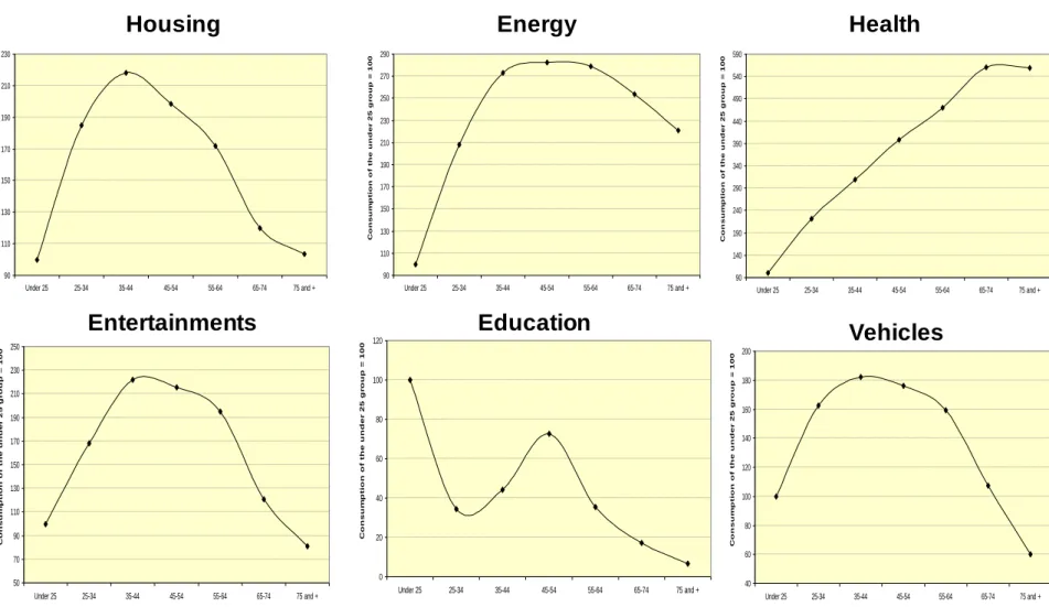
The first fact relates to consumption structure and how it evolves with age. Household survey data allow an assessment of the age-group specific composition of consumption expenditure by broad categories of goods and services. Figure 3 shows the relative level of consumption for main items and age group for the US. Most expenditure items display a hump-shaped profile. The consumption level per capita increases steadily with age, peaks at middle-age then decreases. Only health consumption increases with age. The same profiles can be observed for other countries (cf. Oliveira Martins et al., 2005).

[Figure 3. Relationship between age and consumption by expenditure items in the US] While health care is one the few consumption items increasing with age,11 it is also heavily subsidised. The shares of publicly provided health services to household income increased steadily countries (e.g. France, Sweden, UK and USA, see Figure 4). The ratios varying from 5-7% of household income in UK and US to 10-15% in France and Sweden.

[Figure 4. Ratio of Public Health Expenditure to Household income]

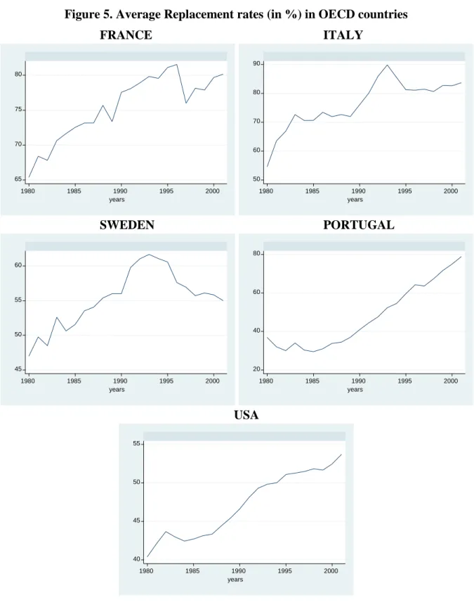
At the same time, average replacement rates increased in most countries (Figure 5).12 For example, in France, Italy and Portugal they reached above 80%. In US, starting from a lower basis they reached close to 55% in the early 2000s. In Sweden they have declined following pension reform to around 55%. By 2003, average replacement rates in PAYG systems are around 58% compared with 44% in fully-funded systems. As many PAYG systems are currently unsustainable, this should induce a decline in replacement rates over time.

[Figure 5. Average replacement rates in OECD countries]

11. Note that age by itself is not a major driver of health care expenditures, but other factors such as the proximity to death, the effects of income and technological progress. In contrast, the expenditures of long-term care are mainly determined by the age profile (see Oliveira Martins and de la Maisonneuve, 2007 for a discussion). 12. Average replacement rates are defined here as the ratio between average pension benefits to gross average

How the interrelations among these basic facts can explain the puzzles? The changing structure of consumption with age, together with a large subsidy for welfare goods and increasing replacement rates could provide an explanation for both the ageing-consumption and ageing-saving puzzles. If old-age consumers shift their consumption structure towards goods that are heavily subsidised and receive substantial retirement income, this could both induce a decline of observed consumption expenditures and a surplus of saving at older ages. This hypothesis will be tested in the next section. To investigate how the saving rates are related to the introduction of fully-funded systems, we ran a simple regression of household saving13 rates (SAVit) on the rate of capitalisation (CAPit, defined as

the ratio of pension fund assets on GDP) for a set of 25 OECD countries for the period 1993-2005. We use both an OLS pooled regression and a fixed-effect model. To avoid a potential endogeneity problem, the capitalisation variable is lagged by one period. Results are as follows:

193 ) .40 4 -( _ _ 12 . 0 4 . 11 193 ) 72 . 4 -( 47 . 0 23 . 9 1 , 1 ,                N t student effects Fixed Country Cap Sav N t student Cap Sav it t i it it t i it  

Capitalisation appears negatively correlated to saving rates. As our theoretical model suggests that PAYG systems should display lower not higher saving rates (cf. Figure 2 above), this is a saving-capitalisation puzzle. A possible explanation could be related to compensation between private and public savings or Ricardian equivalence (Barro, 1974). When government budgets are running on debt or public pension systems are not sustainable, households anticipate a required increase in future taxes and/or lower transfers and adjust their current level of savings accordingly. To check this point, we split our sample in two groups of countries: those offering a large coverage by PAYG and those having large fully-funded systems. The latter group include Australia, Canada, Denmark, Ireland, Netherlands, Switzerland, the UK and the US. All these countries have private pension assets close or above 100% of GDP.

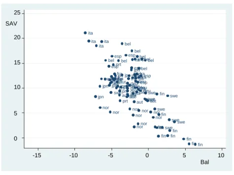
In both groups, the countries with the largest budget deficits also display the largest saving rates (Figure 6). The relationship is particularly strong for the countries dominated by PAYG systems.

[Figure 6. Public budget balances and Saving rates]

Now, if we run the same regressions for the sub-set of OECD countries with fully-funded systems we obtain the following results:

13. Household saving is defined here as household disposable income less consumption. Household income consists primarily of the compensation of employees, self-employment income, and transfers. Property and other income - essentially dividends and interest - are evaluated in the light of business income and debt interest flows. The sum of these elements is adjusted for direct taxes and transfers paid to give household disposable income. Note that SNA93/ESA95 has changed the concept of disposable income for households (compared with SNA68/ESA79) so as to include private pension benefits and subtract private pension contributions.

65 ) 55 . 4 ( _ _ 12 . 0 9 . 12 65 ) 45 . 5 ( 84 . 0 06 . 0 1 , 1 ,                 N t student effects Fixed Country Cap Sav N t student Cap Sav it t i it it t i it  

The OLS pooled regression model shows a positive impact between capitalisation and saving ratios. However, the introduction of fixed-effects changes the sign of the capitalisation coefficient. In other words, within countries, the increase in capitalisation is concomitant with a decrease in saving rates. A possible way to reconcile this result with our model would be to take into account the widespread increase of replacement rates, noted above. Despite the introduction of fully-funded systems, the latter could still induce a decline in savings.

5. Revisiting the ageing puzzles: empirical tests

Drawing from the above results, we are now in a position to test a reduced-from model embodying both the long-term determinants of the saving rates suggested by the theoretical model, as well as other determinants. The specification accounts for a variety of saving determinants identified in the literature (e.g. Edwards, 1996; Loayza, Schmidt-Hebbel and Serven, 2000; Musalem 2004). The list is as follows:

(i) Short-term and macroeconomic determinants: - Public budget balance (in % GDP)

- GDP per capita growth - Long term real interest rate

(ii) Social security and welfare systems determinants:

- Ratio of Public health expenditures on Household income14 (proxy for the provision of welfare goods)

- Average replacement rate (in public and private pension systems)15

(iii) Structure of the population:

- Shares of prime (25-59) and old-age (60+) population - Ratio of life expectancy at 60 to life expectancy at birth16

14. Note that the ratio to household income is a better measure of the amount of transfers than GDP, as the latter by definition does not include the PAYG income.

15. We used this variable because it the only available for a large sample of countries and years. A better proxy could eventually be the replacement rate of the retiring cohort in each year.

To test for the hypothesis discussed above, we also introduced interaction terms. The first term is the product of public health spending ratio with the replacement rate. This captures the combined effect of the subsidization of health goods and pension income. By creating an excess income at older ages, it is expected to have a positive sign on total household savings. The second term is the product of the replacement rate by the share of the old population. While a high replacement rate may discourage saving for the active population, it may also contribute to generate excess income after retirement.

The empirical test covers 18 OECD countries17 and the period 1970-2003. Annex 1 provides descriptive statistics on the different variables used in the regressions. The estimates were carried out using country fixed-effects. A time trend captures an eventual spurious correlation among saving rates and explanatory variables (alternative specifications are also provided in Annex). We also present separate regressions for the sub-set countries with mainly PAYG and fully-funded systems. 18

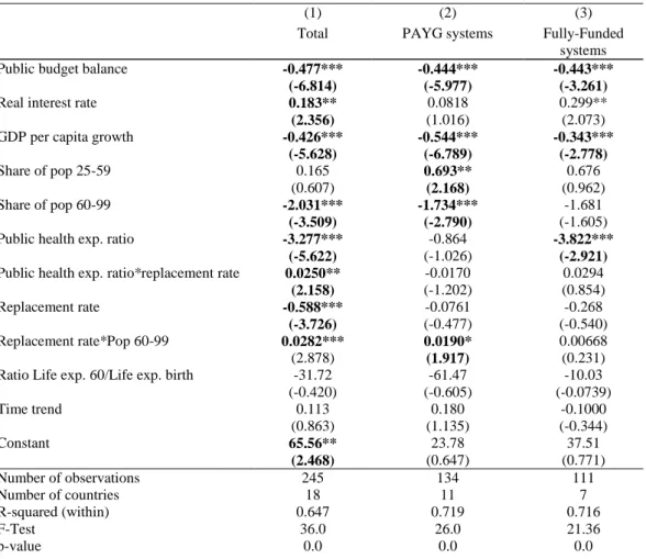
[Table 1. Econometric estimates of household saving rate]

Most estimated coefficients are significant and have the expected sign (Table 1). The level of the public budget balance has a negative impact on savings, i.e. budget deficits tend to increase the saving rates. Among others, this result is compatible with the Ricardian equivalence, although the size of the estimated coefficient is below one indicating that there is no full compensation between public and private savings.19 This helps explaining the saving-capitalisation puzzle, as suggested above.

The real interest rates impact positively saving rates, though the former not being significant in PAYG countries. The coefficient of GDP per capita growth is negative. But this control has often an ambiguous sign in saving equations. In line with the life-cycle model, an increase in the share of old-age population (60-99 years) has a strong negative impact on the saving rate for the total sample and for the PAYG systems. The share of prime-age population (25-59 years) is only significant for PAYG countries.

More importantly, in accordance to our theoretical framework, the generosity of pension systems and subsidisation of health goods impact negatively on saving rates. Both the Public health expenditure ratio and the average replacement rate have negative and significant coefficients for the overall sample. The magnitude of the effects for the health transfers is large. An increase of one percentage point of public health spending ratio to household income induces on average a decrease of

16. As noted above, in the context of our two-period life-cycle model, the survival probability can be defined as the ratio of the numbers of years in retirement (period 2) to the numbers of years in period 1 (taken at 60 years). It is then straightforward to see that the term pi/(1+pi) in equation (13) is equal to ratio of life

expectancy at 60 divided by the life expectancy at birth.

17. Unfortunately, not all variables were available to all OECD countries thus the sample had to be restrained to Australia, Austria, Belgium, Canada, Denmark, Germany, Finland, France, Italy, Japan, Netherlands, Norway, Poland, Portugal, Spain, Sweden, UK and the US.

18. PAYG systems: Austria, Belgium, Germany, Finland, France, Italy, Japan, Norway, Portugal, Spain and Sweden; Fully-funded systems: Australia, Canada, Denmark, Netherlands, Switzerland, UK and the US. 19. This is line with other empirical results in the literature (e.g. Serres and Pelgrin, 2003; de Mello, Kongsrud

1.7 percentage points in the household saving rate (ranging from 0.5 to 2.5 percentage points in the sample).20 In contrast, the combined effect of the replacement rate is rather small.

The estimates also show that larger health transfers combined with pension income has a positive impact on the saving ratio. This helps explaining the ageing-saving puzzle. The interaction between replacement rates and the share of old-age population has also a positive impact on savings. This result is compatible with the fact that old-aged households could display excess income when there is no perfect consumption smoothing (see footnote 10).

Finally, the sign of the life expectancy ratio is negative but not significant. This is compatible with equation (11) above, showing that the impact of survival probability on savings is not monotonic. The time-trend is also not significant. In annex additional specifications were also carried out, basically confirming the results from the base specification.

6. Concluding remarks

Some empirical facts on consumption, pension and saving do not fit well with theory. Four types of puzzles have emerged: an ageing-consumption, an ageing-saving, a saving-capitalisation and a saving-longevity puzzle. While most studies in the literature have analysed these puzzles separately, the originality of this paper is to integrate these four puzzles together. We developed a life-cycle theoretical model. Inspired from this model and a number of other determinants of savings analysed in the literature, we then estimated a reduced-form econometric model.

Our empirical results show that the four puzzles are linked together. The changing structure of consumption with age, together with a large subsidy for welfare goods and increasing replacement rates provides an explanation for both the ageing-consumption and ageing-saving puzzles. If old-age consumers shift their consumption structure towards goods that are heavily subsidised and receive increased retirement income, this induces a decline of consumption and a surplus of saving at older ages. Accordingly, higher replacement rates and larger public provision of health care contribute negatively to the savings rate. Furthermore, the level of the public budget balance has a negative impact on savings. This explains the observed saving-capitalisation puzzle. Finally, in line with standard life-cycle effects, we also showed that an increase in the share of the old-age population has a strong negative impact on the saving rate.

Finally, concerning the longevity-saving puzzle, our estimates did not provide significant results. Nonetheless, our theoretical model can explain why with large replacement rates an increase of the survival probability may induce a negative effect on savings.

References

Ando A. and F. Modigliani (1963), “The Life Cycle Hypothesis of Saving: Aggregate Implications and Tests”, American Economic Review 53, 55-84.

Arellano, M. and S. Bond (1991), “Some tests of specifications in Panel data: Monte Carlo evidence and an application to employment equations”, Review of Economic Studies 58: 277-297.

Attanasio, O.P. (1999), “Consumption”, in Handbook of Macroeconomics, Vol. 1B, edited by J. Taylor and M. Woodford, Amsterdam: Elsevier Science.

Baillu J. and H. Reisen (1997), “Do Funded Pensions Contribute to Higher Aggregate Savings? A Cross Country Analysis”, OECD Development Centre Technical Papers 130.

Banks J., Blundell R. and S. Tanner (1998), “Is There a Retirement-Savings Puzzle?” American

Economic Review, 88 (4), 769-788.

Barro R. (1974), “Are Government Bond Net Health ?”, Journal of Political Economy, 81, 1095-1117.

Bernheim D., Skinner J. and S. Weinberg (2001), “What Accounts for the Variation in Retirement Wealth among U.S. Households?” American Economic Review, 91 (4), 832-857.

Bloom D., Canning D. and B. Graham, (2003), “Longevity and Life-Cycle Savings”, Scandinavian

Journal of Economics 105, 319–38.

Bloom D., Canning D., Mansfield R. and M. Moore, (2006), “Demographics Change, Social

Security Systems and Savings”, NBER Working Paper no. 12621,

http://www.nber.org/papers/w12621

Bohn H., (1999), “Social Security and Demographic Uncertainty: The Risk Sharing Properties of Alternative Policies”, WP, University of California of Santa Barbara.

Börsch-Supan A., A. Reil-Held, R. Rodepeter, R. Schnabel and J. Winter (2000), “The German Savings Puzzle”, Universitat Mannheim Working Paper No. 01-07.

Börsch-Supan, A. H. and J. K. Winter (2001), “Population Aging, Savings Behavior and Capital Markets”, NBER Working Paper no. 8561.

Borsworth B. and G. Burtless (2004), Pension Reform and Saving, The Brookings Institution.

Chakraborty S., (2004), “Endogenous lifetime and economic growth”, Journal of Economic Theory, N°116, pp119-137.

Corsetti G., K. Schmidt-Hebbel, (1995), “Pension Reform and Growth”, The World Bank Policy

Reform Working Paper No. 1471, Policy Research Department.

Drouhin, N. (2002), « Inégalités face à la mort et systèmes de retraite », Revue d’Economie

Politique, 111-126.

Drouhin, N. (2000), « Statique Comparative du modèle de choix intertemporel avec durée de vie incertaine : le cas discret », Notes de Recherche du GRID, no. 00-20.

Edwards S. (1996), “Why are Latin America‟s Saving Rates So Low? An International Comparative Analysis”, Journal of Development Economics 51, 5-44.

Federal Reserve Board, Flows and Funds Accounts, various years, Federal Reserve, Washington, DC.

Feldstein M. (1974), “Social Security, induced retirement and aggregate capital accumulation”,

Journal of Political Economy 82, 905-26.

Feldstein, M. (1996), “Social Security and Savings: New Time Series Evidence”, National Tax

Journal 49, 151-164.

Fernandez-Villaverde, J. and D. Krueger (2002), “Consumption Over the Life Cycle: Some Facts from Consumer Expenditure Survey Data”, PIER Working Paper 02-44.

Friedman, M. (1957), The Theory of the Consumption Function, Princeton University Press, Princeton (New Jersey).

Hurd M. and Rohwedder S. (2006), “Some answers to the Retirement-Consumption Puzzle”, NBER

Working Paper No. 12057, http://www.nber.org/papers/w12057.

Hurd M. and S. Rohwedder (2003), “The Retirement-Consumption Puzzle: Anticipated and Actual Declines in Spending at Retirement”, NBER Working Paper No. 9586.

Jørgensen, H. and S. Jensen (2008), “Labour supply and Retirement Policy in an Overlapping Generations Model with Stochastic Fertility”, CEBR Discussion Paper.

Khitatrakun S. and Scholz J.K. (2004), “Are Americans Saving "Optimally" for Retirement?” NBER

Working Paper No. 10260.

Loayza N., Klaus Schmidt-Hebbel K. and L. Servén (2000), “What Drives Private Saving across the World?”, The Review of Economics and Statistics, Vol. 82, No. 2. May, 165-181.

Loayza, N., Lopez, H., Schmidt-Hebbel K., and L. Serven (1998), The World Saving Database, World Bank manuscript, The World Bank, Washington, DC.

de Mello, L., P.M. Kongsrud, and R. Price (2004), “Saving Behaviour and the Effectiveness of Fiscal Policy”, OECD Economic Department Working Papers No. 397.

Modigliani, F. and R. Brumberg (1954), “Utility analysis and the consumption function: an interpretation of cross-section data”, in Post-Keynesian economics, (ed.) K. Kurikara, Rutgers University Press.

Moore J. F. and O. Mitchell (1998), “Can Americans Afford to Retire? New Evidence on Retirement Saving Adequacy”, The Journal of Risk and Insurance, Vol. 65, No. 3, pp. 371-400.

Murphy P. L. and A. R. Musalem, (2004), “Pension Funds and National Saving”, The World Bank

Working paper Series No. 3410, Washington, DC.

OECD, Institutional Investors, various years, OECD.

Oliveira Martins, J., F. Gonand, P. Antolin, C. de la Maisonneuve and K. Yoo (2005), “The Impact of Ageing in Demand, Factor Markets and Growth”, OECD Economics Department Working Papers No. 420.

Oliveira Martins, J. and C. de la Maisonneuve (2006), "The Drivers of Public Expenditure on Health and Long-Term Care: an Integrated Approach", OECD Economic Studies no. 43/2.

Serres, A. and F. Pelgrin (2003), “The decline of Private Saving rates in the 1990s in OECD countries: How much can be explained by non-Wealth Determinants”, OECD Economic Studies No. 36, 2003/1.

Sheshinski, E. (2004), “Longevity and Aggregate Savings: Comment”, Hebrew University of Jerusalem, mimeo.

Smith (2007), “Can the retirement-consumption puzzle be resolved? Evidence from UK panel data”,

The Institute for Fiscal Studies Working Paper No. 04/07.

Yaari, M. (1965), “Uncertain Lifetime, Life insurance and the Theory of the Consumer”, Review of

Figure 1. The Consumption-Saving Puzzle United States 80.0 100.0 120.0 140.0 160.0 180.0 200.0 220.0 under 25 25-34 35-44 45-54 55-64 65-74 75 + C o n s u m p ti o n o f th e u n d e r 2 5 a g e g r o u p = 1 0 0 European countries 40.0 60.0 80.0 100.0 120.0 140.0 160.0 180.0 under 30 30-44 45-59 60 + C o n s u m p ti o n o f th e u n d e r 3 0 a g e g r o u p (EU a v e r a g e ) = 1 0 0 Fin Swe Deu Gbr Ita Fra

Source: Consumer Expenditure Survey, US, 2002; Household Budget Survey of Eurostat and Luxembourg Income Study.

Figure 2. The Saving-Capitalisation Puzzle

Average Household Saving rate

0.0 2.0 4.0 6.0 8.0 10.0 12.0 14.0 16.0 18.0 1989 1990 1991 1992 1993 1994 1995 1996 1997 1998 1999 2000 2001 2002 2003 2004 2005 2006 Low Funding High Funding

Figure 3. Relationship between age and consumption by expenditure items in the US 90 110 130 150 170 190 210 230 Under 25 25-34 35-44 45-54 55-64 65-74 75 and + C o n s u m p t io n o f t h e u n d e r 2 5 g r o u p = 1 0 0 90 110 130 150 170 190 210 230 250 270 290 Under 25 25-34 35-44 45-54 55-64 65-74 75 and + C o n s u m p t io n o f t h e u n d e r 2 5 g r o u p = 1 0 0 50 70 90 110 130 150 170 190 210 230 250 Under 25 25-34 35-44 45-54 55-64 65-74 75 and + C o n s u m p t io n o f t h e u n d e r 2 5 g r o u p = 1 0 0 0 20 40 60 80 100 120 Under 25 25-34 35-44 45-54 55-64 65-74 75 and + C o n s u m p t io n o f t h e u n d e r 2 5 g r o u p = 1 0 0

Housing

Energy

Entertainments

Education

Health

Vehicles

NB: Consumption levels per capita in each age group are normalised at 100 to the under 25 years age group. Source: Consumer Expenditure Survey, US, 2002.

Figure 4. Ratio of Public Health Expenditures to Household income 0 5 10 15 in % 1970 1980 1990 2000 France UK Sweden USA

Figure 5. Average Replacement rates (in %) in OECD countries

FRANCE ITALY

SWEDEN PORTUGAL

USA

Source: OECD ADB data base and authors‟ calculations.

50 60 70 80 90 1980 1985 1990 1995 2000 years 65 70 75 80 1980 1985 1990 1995 2000 years 45 50 55 60 1980 1985 1990 1995 2000 years 20 40 60 80 1980 1985 1990 1995 2000 years 40 45 50 55 1980 1985 1990 1995 2000 years

Figure 6. Public budget balances and Saving rates PAYG systems

Fully-funded systems

Legend: SAV: household saving rates (in % of Household income); Bal: Public budget balance (in % of GDP).

Source: OECD National Accounts and ABD database. aut

aut aut

aut aut autautaut

aut aut bel bel bel bel bel bel bel bel deu deu deu_deu deudeu deu deu deu deu esp esp esp esp esp esp esp esp fin fin fin fin fin fin fin fin fin fin fra fra fra fra fra fra_fra fra fra ita ita ita ita ita ita ita ita ita jpn jpn jpn jpnjpn jpn jpn jpn nor nor nor nornor nor_nor nor nor prt prt prt prt prt prt sweswe swe swe swe swe swe swe swe swe 0 5 10 15 20 25 SAV -15 -10 -5 0 5 10 Bal aus aus aus aus aus aus aus aus aus aus can can _can can can can can can can can chechecheche

cheche che che dnk dnk dnk dnk dnk dnk dnk gbr gbr gbr gbr gbr gbr gbr gbr nld nld nld nld nld nld usa usa_usa usa usa usa usausa usa usa -5 0 5 10 15 SAV -15 -10 -5 0 5 Bal

TABLE 1. Econometric estimates of household saving rate1

(1) (2) (3)

Total PAYG systems Fully-Funded systems

Public budget balance -0.477*** -0.444*** -0.443***

(-6.814) (-5.977) (-3.261)

Real interest rate 0.183** 0.0818 0.299**

(2.356) (1.016) (2.073)

GDP per capita growth -0.426*** -0.544*** -0.343***

(-5.628) (-6.789) (-2.778)

Share of pop 25-59 0.165 0.693** 0.676

(0.607) (2.168) (0.962)

Share of pop 60-99 -2.031*** -1.734*** -1.681

(-3.509) (-2.790) (-1.605)

Public health exp. ratio -3.277*** -0.864 -3.822***

(-5.622) (-1.026) (-2.921)

Public health exp. ratio*replacement rate 0.0250** -0.0170 0.0294

(2.158) (-1.202) (0.854)

Replacement rate -0.588*** -0.0761 -0.268

(-3.726) (-0.477) (-0.540)

Replacement rate*Pop 60-99 0.0282*** 0.0190* 0.00668

(2.878) (1.917) (0.231)

Ratio Life exp. 60/Life exp. birth -31.72 -61.47 -10.03

(-0.420) (-0.605) (-0.0739) Time trend 0.113 0.180 -0.1000 (0.863) (1.135) (-0.344) Constant 65.56** 23.78 37.51 (2.468) (0.647) (0.771) Number of observations 245 134 111 Number of countries 18 11 7 R-squared (within) 0.647 0.719 0.716 F-Test 36.0 26.0 21.36 p-value 0.0 0.0 0.0

(1) Defined as household saving on household income. All models include country Fixed-effects (not reported). T-statistics are in parentheses, *** p<0.01, ** p<0.05, * p<0.1. The Hausman specification test of the fixed-effects vs. the random-effect model is also provided (p-values in parenthesis indicate the fixed-effect cannot be rejected at 95% confidence level).

PAYG systems: Austria, Belgium, Germany, Finland, France, Italy, Japan, Norway, Portugal, Spain and Sweden; Fully-funded systems: Australia, Canada, Denmark, Netherlands, Switzerland, UK and the US.

Annex 1: Descriptive statistics of the variables used in the econometric estimates

Variable Obs Mean Std. Dev. Min Max

Household saving ratio _{612 10.08 6.26 -12.82 30.23}

Public budget balance _{529 -2.78 3.45 -16.38 7.84}

Real interest rate _{599 3.05 3.64 -17.82 14.25}

GDP per capita growth _{675 2.18 2.37 -9.16 10.70}

Share of pop 25-59 _{507 46.08 2.89 37.44 51.79}

Share of pop 60-99 _{522 16.76 3.10 10.53 24.85}

Public health exp. ratio _{535 9.39 2.68 3.13 16.22}

Public health exp. ratio*replacement

rate 329 526.20 181.14 194.71 961.48

Replacement rate _{392 52.61 13.78 28.78 89.87}

Replacement rate*Pop 60-99 _{355 929.74 347.44 369.78 2007.54} Ratio Life exp. 60/Life exp. birth _{681 0.26 0.01 0.23 0.30}

Annex 2: Sensitivity Analysis with alternative econometric estimates

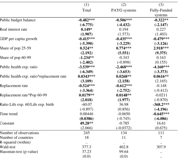
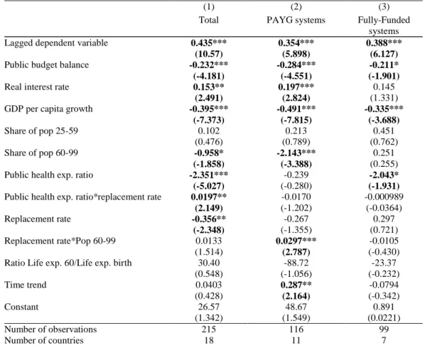
In order to test the sensitivity of the results to alternative specifications, we also carried out estimates using the random-effect model (Table A.1) and the dynamic panel estimator using the Arellano-Bond (1991) method (Table A.2). Note that, according to the Hausman test, the random-effect model is not accepted against the fixed-effect model (our preferred specification).

In general, the signs of estimated coefficients are robust. The long-term real interest rate, the GDP per capita growth and public budget balance keep the same signs and roughly the same magnitudes. The share of old-age (60+) population also remains negative, while the effect of the share of prime-age populations is positive. The health expenditure ratio (the proxy for the provision of welfare goods) is robustly negative, as well as the replacement rate. The interaction terms are also robust as they display the same signs as in the base specification. The coefficient on the relative life expectancy only appears negative in the case of the random-effect panel and for funded systems.

TABLE A.1 Econometric estimates of household saving rate, Random-effect model1

(1) (2) (3)

Total PAYG systems Fully-Funded systems

Public budget balance -0.482*** -0.506*** -0.322**

(-6.775) (-4.432) (-2.147)

Real interest rate 0.149* 0.194 0.227

(1.907) (1.573) (1.403)

GDP per capita growth -0.415*** -0.435*** -0.479***

(-5.390) (-3.229) (-3.126)

Share of pop 25-59 0.524** 0.774*** 2.918***

(2.192) (5.551) (9.375)

Share of pop 60-99 -1.234** -0.343 0.163

(-2.402) (-0.898) (0.155)

Public health exp. ratio -3.539*** -2.468*** -4.160***

(-6.349) (-3.653) (-3.373)

Public health exp. ratio*replacement rate 0.0343*** 0.0268** 0.0616**

(3.109) (2.158) (2.165)

Replacement rate -0.524*** -0.612*** -0.148

(-3.364) (-2.752) (-0.412)

Replacement rate*Pop 60-99 0.0179** 0.0148** -0.0211

(2.018) (1.977) (-0.870)

Ratio Life exp. 60/Life exp. birth -60.07 36.98 -368.2***

(-0.897) (0.856) (-4.196) Time trend 0.00446 -0.0650 -0.645*** (0.0386) (-0.745) (-6.086) Constant 49.28** -0.785 16.61 (2.066) (-0.0372) (0.675) Number of observations 245 134 111 Number of countries 18 11 7 R-squared (within) .. .. .. Wald-test 377.3 402.8 307.9 Hausman-test (p-value) 37.23 99.64 .. (0.0) (0.0) ..

(1) Defined as household saving on household income. T-statistics are in parentheses, *** p<0.01, ** p<0.05, * p<0.1. The Hausman specification test of the fixed-effects vs. the random-effect model is also provided (p-values in parenthesis indicate the fixed-effect cannot be rejected at 95% confidence level). PAYG systems: Austria, Belgium, Germany, Finland, France, Italy, Japan, Norway, Portugal, Spain and Sweden; Fully-funded systems: Australia, Canada, Denmark, Netherlands, Switzerland, UK and the US.

TABLE A.2 Econometric estimates of household saving rate, Dynamic Panel estimates1

(1) (2) (3)

Total PAYG systems Fully-Funded systems

Lagged dependent variable 0.435*** 0.354*** 0.388***

(10.57) (5.898) (6.127)

Public budget balance -0.232*** -0.284*** -0.211*

(-4.181) (-4.551) (-1.901)

Real interest rate 0.153** 0.197*** 0.145

(2.491) (2.824) (1.331)

GDP per capita growth -0.395*** -0.491*** -0.335***

(-7.373) (-7.815) (-3.688)

Share of pop 25-59 0.102 0.213 0.451

(0.476) (0.789) (0.762)

Share of pop 60-99 -0.958* -2.143*** 0.251

(-1.858) (-3.388) (0.255)

Public health exp. ratio -2.351*** -0.239 -2.043*

(-5.027) (-0.280) (-1.931)

Public health exp. ratio*replacement rate 0.0197** -0.0170 -0.000989

(2.149) (-1.202) (-0.0364)

Replacement rate -0.356** -0.267 0.297

(-2.348) (-1.355) (0.721)

Replacement rate*Pop 60-99 0.0133 0.0297*** -0.0105

(1.514) (2.787) (-0.430)

Ratio Life exp. 60/Life exp. birth 30.40 -88.72 -23.37

(0.548) (-1.056) (-0.232) Time trend 0.0403 0.287** -0.0794 (0.428) (2.164) (-0.342) Constant 26.57 48.67 0.891 (1.342) (1.549) (0.0221) Number of observations 215 116 99 Number of countries 18 11 7

(1) Defined as household saving on household income. Regressions were carried out using the dynamic Arellano-Bond estimator. T-statistics are in parentheses, *** p<0.01, ** p<0.05, * p<0.1.

PAYG systems: Austria, Belgium, Germany, Finland, France, Italy, Japan, Norway, Portugal, Spain and Sweden; Fully-funded systems: Australia, Canada, Denmark, Netherlands, Switzerland, UK and the US.