1
T
HE
C
HOICE OF AN
O
PTIMAL
E
XCHANGE
R
ATE
R
EGIME
FOR THE
E
URO
CFA
C
OUNTRIES
Z
ONE
authored by MIREILLE LINJOUOM
CONTENTS
SECTION I: INTRODUCTION... 1
SECTION II: THE THEORETICAL MODEL... 3
2.1 The supply side... 4
2.2 The demand side... 4
SECTION III:THE MODEL OF THE CHOICE OF AN EXCHANGE RATE REGIME... 5
3.1 the credibility of the pegged regime as a rule... 9
3.2 the discretionary policy under flexible exchange rate regime... 10 3.3 Welfare comparison of the two exchange rate regime... 13
SECTION IV:PEGGED BUT ADJUSTABLE VERSUS FLEXIBLE EXHANGE RATE REGIME ... 15
4.1Sources and measures of political instability... 15
4.2 the loss function under flexible and fixed and adjustable exchange rate regimes ... 16
4.3 decisions rules basis for the choice of an exchange rate regime... 18
CONCLUSION... 21
TABLES 1.A simple small open economy model……….... 4
2.Optimization program……….………... 8
FIGURES 1. Timing of events... 8
3
I.INTRODUCTION
The individual countries’ decision to adopt a particular exchange rate arrangement depends on many considerations. Following the collapse of the Bretton Woods System of fixed exchange rate in 1973, most developing countries continued to peg the value of their currency to the currency of their main trading partner. Since then, most of them have evolved towards greater flexibility arrangement, consisting particularly on managed exchange rate regimes. According to the IMF’s International Financial Statistics, the number of developing countries still adopting a pegged exchange rate arrangement decreased from 81 percent in 1976 to 43 percent in 1998. Exchange rate flexibility is being increasingly adopted as an adjustment process instrument in a world economy undergoing increasing international integration and in some respects, increased potential instability. Despite this trend, the economies of the Euro CFA zone have continued to maintain the pegged regime first adopted in 1948, throughout 1994 when the CFA franc was devalued.
The Euro CFA zone comprises 14 sub-Saharan African countries, of which 12 former French colonies. Formally, they are divided into two currency unions, sharing their respective single currencies (which have the same acronym , CFA franc) issued by two regional central banks, located in Dakar (Senegal) and Yaounde (Cameroon). The two currencies are, by definition, pegged to the French franc and thus now to the Euro. The Euro CFA zone is unique in the world as a monetary union with a fixed exchange rate to the anchor currency country, France, guarantees the convertibility of the CFA Franc into French franc/Euro. France participates in the executive boards of the two regional central banks, and provides extensive financial and technical assistance to the member countries of the zone.
After more than 40 years of stability, the 50 percent devaluation of the CFA franc in January 1994, as well as influential factors, such as the European Monetary Union construction affect the performance of the Euro CFA zone, among other, through the degree of variability of the Euro exchange rate to the dollar. Moreover, these me mber countries are confronted with a series of external disturbances resulting from the step rise in international interest rate, the adverse terms of trade movements and the debt crisis. In view of this situation, the arising issue is whether the Euro CFA countries should abandon the current pegged exchange rate arrangement and adopt a more flexible regime. The trade-off involved is justified since those countries must face external factors as well as internal ones derived, among others, from political considerations and domestic inflationary pressures resulting from public finance deficits leading to overvalued domestic currency.
An extensive theoretical literature is available on the optimum choice of an exchange regime. The first approach is based on the theory of the optimal currency area which focuses on a country’s economic structural characteristics, so as to determine whether it would be better off in terms of its ability to maintain external and internal balance through a fixed as compared to a flexible exchange arrangement. Subsequent discussions originating in the 1960s by Mundell (1961) focused on the optimal exchange regime to maintain external balance, while McKinnon (1962) emphasized maintenance of price stability. The main conclusions of that literature are that a small open economy is better served by a fixed exchange rate. However, the more diversified is a country’s production and export structure and the less geographically concentrated its trade, the stronger is the case for the flexible exchange rate regime. This arrangement is also attractive for the case of lower degrees of factor mobility, higher divergence of domestic inflation from that of its main trading partner and higher level of economic and financial development.
The second approach relies on a large theoretical literature that examined the optimal choice of an exchange regime so as to stabilize macroeconomic in a world subject to different types of shocks. The basic conclusion of these studies is that the optimal choice of an exchange regime depends on the nature and size of these shocks as well as the structure of the economy (see for example Fisher (1977), Turnovsky (1977), Flood (1979), Frenkel and Aizenman (1982). These analyses show that if the disturbances are foreign and domestic real shocks such as shift in the demand of domestic goods, and even foreign nominal shocks, a greater degree of flexibility is preferable. But when the country experiences domestic nominal shocks, an exchange rate adjustment is not necessary.
A third and most recent approach emphasizes the role of credibility and political factors in the rational process to select an exchange regime. For extensive reviews and discussions see for example Aghevli, Moshin, and Montiel (1991), Edwards and Tabellini (1994), Collins (1996), Edwards (1996), Agénor and Montiel (1998). The main point of this literature is to stress that it may be politically costlier to adjust a pegged exchange rate than to allow the nominal exchange rate to fluctuate by a correspond ing amount in a more flexible exchange rate arrangement. In a flexible regime, any modification in the nominal exchange rate may neither be easily appreciated nor clearly reflect government decisions, as it would be the case if the currency was depreciated. This implies that the decision to adopt flexible exchange rate is partly taken to “de-politicize” exchange rate adjustments.
The main conclusion on these approaches is that the rational process to select an exchange regime for a developing country depends on the structural characteristics of its economy, the nature and source of the schocks as well as political considerations. Following this conclusion remark, the paper develops an analytical framework allowing to proceed to the definition of an optimal exchange regime for the Euro CFA countries. Indeed, the experience of this zone illustrates the main trade-off involved in the choice of an exchange rate regimes. Despite, the 1994 devaluation from a fixed rate of 50 to 100 CFA francs per French franc, the members countries of this zone still continued to commit themselves to a fixed rate regime, to anchor their price levels and maintain inflation close the rate experienced in Europe through French Treasury management, whose currency served as the peg. Such a policy resulted in a loss of their ability to adjust to external shocks on the domestic economy. Indeed by selecting a flexible regime, they would have been able to limit the damage caused by the volatility of their main tradable goods in the world markets and of the international interest rate.
The paper is organized as follows. Section II describes a typical small open developing country which produces tradable as well as semi- tradables goods and that is affected by external shocks. Section III considers policy makers’ preferences that behave strategically to decide whether to adopt an irrevocably fixed or a flexible exchange rate regime. The model assumes that the authorities minimize a quadratic loss function that capture the trade-off between inflation an real growth in the tradable sector. The authorities' decision process takes into account and compare the expected value of a quadratic loss function under alternative exchange rate regimes. Section IV extends the model by considering political factors. As a pegged exchange rate regime can not be permanently fixed, the policy makers have to choose between intermediate exchange rate arrangements such as a fixed but adjustable and a flexible managed exchange rate regime. Section V offers some concluding remarks.
5
II. THE THEORETICAL MODEL
This section present a simple static log- linear model of a small open economy which will serve as the basis for discussion of alternative exchange rate regimes. This simple model constitutes the basic framework used for the analytical discussions on the optimal exchange management.
2.1 The supply side
The model set is a distillation of the dependent economy of Swan (1963). This is a simple model of a small open economy which produces both tradable and semi-tradable goods. This production structure relaxed the constraint that is imposed by the small country assumption. Owing to its relative small size the country is price-taker in the world market of tradable goods and the export sector is the traditional, price–taking sector. The rest of the economy produces a semi- tradable good which is imperfectly substitutable with the imported commodity (Devarajan and De Melo (1987)).
The whole country’s production is assumed to cover the two sectors:
ST T+y =y
y (1)
where y is the logarithm of the output, yT is the logarithm of the production of tradable goods and yST is the logarithm of the production of semi-tradable goods.
Following the models in Barro and Gordon (1983), Devarajan and Rodrik (1992), Edwards (1996), the equation for the output level in the tradable sector, yT, is expressed as follow:
x x y y ( - ) ( -ST T T T= +λ π π +µ ) (2)
whereyT is the logarithm natural level of tradable output, πT and πST are the logarithm of the differences between the rate of increase in the price of tradables and semi- tradables. (πT-πST) stands for the change in the real exchange rate. x, is a composite variable in logarithm of terms of trade and world interest shocks that show the existence of an income effect whene ver this variable shifts.x is the mean level of the logarithm composite variable x and assumes to have a variance equal to σ². The parameters λ and µ are positive.
Similarly the total output y is determined by two variables, the change in the real exchange rate (πT-πST) and the composite variable x in logarithm of terms of trade and world interest shocks: ) -( ) -( ST T x x y y= +γ π π +φ (3)
where y is the natural level of output, the parameters γ and φ are positive. Equation (2) and (3) state that if the rate of increase in the price of tradables, πT exceeds the rate of increase in the semi-tradables, πST, the real exchange rate raise. This real appreciation reflects an increase in the domestic cost of producing tradable goods and lowers both total and traded output as if external shocks values x were below their mean x .
2.1 The demand side
According to Minford (1998), the whole demand in this low developing country is shared by the demand of tradable goods, DT and the demand of semi- tradable goods, DST:
ST T D D
D= + (4)
The demand curve for tradable goods is determined by two variables, the demand in real terms for traded goods, τD and the change in the real exchange rate (πT-πST):
) -D
DT=τ +η(πT πST (5)
where η is positive, τ =yT/y is a parameter representing the share of the traded output in the
total output with 0<τ<1 .
Equation (4) states that the demand in the semi-tradable sector is the difference between the total demand of goods and the demand for tradable goods and stands as follow:
T ST D-D
D =
The equilibrium in the semi- tradable market is given by:
ST
y
DST= (6)
Equation (7) equate the implied demand for semi-tradable with their output after market-clearing.
Table 1. A simple small open economy model
y = yT+ yST (1) yT= yT + λ ( πT-πST)+ µ (x-x) (2) y =y +γ (πT-πST)+ φ (x-x) (3) D= DT+ DST (4) DT=τD + η( πT-πST) (5) DST= YST (6) D= Y (7)
Where: y=output (in log); y(yT)= natural
level of output (traded output); D(DST) =
demand in real terms (in semi-tradables sector); with parameters γ≥0, φ≥0, α≥0,
β≥0, η≥0 and τ(=yT/y), natural share of
traded output in the total o utput, 0<τ<1; in logarithm: πT-πST=change in real exchange
rate; x= ramdom variable refleting external shocks received by the economy; x = the mean level of external shocks.
7
III.THE MODEL OF THE CHOICE OF AN EXCHANGE RATE REGIME
This section develops a simple theoretical model with policy makers behaving strategically under alternative exchange rate regime in a developing country. This approach relies on the existence of a trade-off between credibility provided by rules that govern economy policy and flexibility allowing the governments to apply discretionary policy after evaluating the situation. It should be made clear that the authorities use discretion to alter the nominal exchange rate. To establish credibility the authorities must convince the public that they are committed to defend the parity which has been clearly defined and stop implementing previously announced policies which would lead to time-inconsistency problems (for a survey on this literature, see for example Barro and Gordon (1983), Persson and Tabellini (1990), Agénor and Montiel (1996)).
A pegged exchange system is assumed to allow the policy makers to resolve, even if partially the time inconsistency problem. It has been argued that the adoption of a fixed exchange rate will constrain the ability of governments to surprise the public through unexpected devaluation.
The Authorities’ Loss Function
Consider the case of a small economy in a developing-country context whose policy makers behave strategically to decide whether to adopt a pegged (permanently) or a flexible exchange rate regime. The authorities' decision process takes into account and compare the expected value of a quadratic loss function under alternative exchange rate regimes.
The authorities are assumed to be interested in minimizing an objective function in both nominal and real intervening variables. The real variable could be the current account, output, or the growth rate. The nominal variable could be the price level or the inflation. The model considers what matters most to policy makers inflation and to develop vested interest in the production of tradable goods, therefore the competitiveness in the tradable sector. The policy makers' preferences are formalized as follow:
L=?
[
(π−π*)²+ϕ(yT−yT*)²]
, ϕ>0 (3.1) where E is the expectation operator, L, the loss function which is quadratic, represents the social costs increase and depends on squared deviations of inflation from a socially optimal target value, π* and on squared deviations of level of output in the tradable sector from a desired target level yT*.The structural economic constraints
The authorities’ behaviour is subject to the constraints imposed by the economy’s structural characteristic and its susceptibility to external shocks.
In section II, the level of output in the tradable sector (in logarithm form) has been set as a function of the level of fluctuation in the real exchange rate (πT-πST) and the external disturbances, x combined with terms of trade and world interest shocks:
y y ( - ) (x-x
ST T
whereyT is the logarithm natural level of traded output. The expected value of the external shocks is represented byx, the mean level of the logarithm composite variable x, with variance σ².
Following Kindland and Prescott (1977), it is assumed that the natural traded output yT is lower than the socially optimal level yT*:
yT*> yT ( 3.3)
where yT* = τy* (y* is the target level of total output and τ=yT/ y represents the natural
share of traded output in total output). Equation (3.3) assumes that the target level of traded output exceeds its natural level. The sub-optimality of the natural level of traded output could be due to pre-existing rigidities in labour market or to various distortions in the taxation (Devarajan and Rodrik, 1992).
The changes in domestic price have to be specified to complete the constraint imposed by the structural characteristics of the economy. It is assumed that the domestic price setters are rational and forward- looking. The price in the semi-traded sector is set so as to protect their position relative to the traded sector and to respond to the exogenous disturbances which affect it. The foreign-currency price of traded goods is determined on world market. The domestic inflation, π, is given by:
T ST ( λ)π
λπ
π = + 1− ( 3.4)
where domestic inflation is a weighted average of the increases in the price of semi-tradables and tradables and (1-δ) is the degree of openness. The domestic price of the tradable sector takes the following form:
πT =d+πTe ( 3.5)
where d represents the rate of devaluation of the nominal exchange rate and eπ , the rate of T increase in the foreign currency price of tradable goods. According to Dornbush (1980), it is assumed for simplicity that the given foreign price is one, it does not fluctuate hence its logarithm is zero and πTe=0. Equation (3.5) becomes the n:
πT=d (3.6)
In assuming that domestic price setters are rational and forward- looking, they react by setting prices in the semi-tradable sector in reaction to fluctuations in the expected domestic price of tradable goods, and to an exogenous shocks in their sector, XN which occurs at the beginning
of the period. Following Agénor and Montiel (1996), the domestic setters’ objective is to minimize their loss function taken to be:
Min
[
d]
N e T a ST P L = π −( +π )−ψΧ 2/2 , ψ>0 (3.a)where da denotes the expected rate of depreciation of exchange rate. After some developing LP the first order condition gives:
=0⇔ −( + )− Χ =0 ∂∂ N e T ST ST P a d L π π ψ π (3.b)
9
The optimal rate of inflation in the semi-tradable sector is N ST a d + Χ = ψ π (3.c)
Under rational expectations, the agents take into account the expected relative price behaviour and the expected external disturbances:
E(d) E(x-x)
ST δ
π = − (3.7)
with a
d =E(d) and ΧN= E(x-x), where E is the operator of the expected value. the timing
therefore suppose that external shocks occurred after the expected changes in domestic price have been set (figure 1) .
Figure 1. Timing of events
Step 1 Step 2 Step 3 Step 4
πST is set the shocks ocurred the authorities set its traded output yT
x is revealed exchange rate policy inflation π are
d is set determined
The sequence of the actions influences the model’s solution. Initially, the agents define under rational expectations the changes in prices in the semi- tradable sector before they observed x,
d, π or yT. The policy makers determine its exchange rate policy, once both πST and x have been revealed.
The authorities’ objective is to set the exchange rate system allowing to minimize the expected value of the loss function given by (3.1).
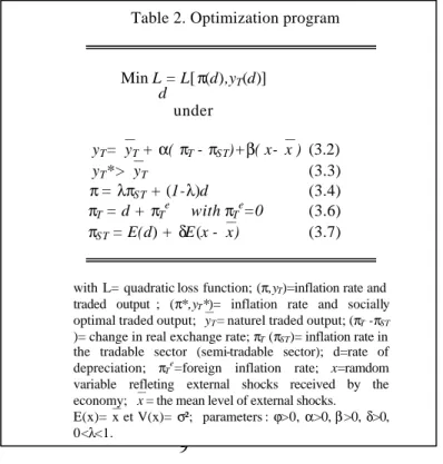
Table 2. Optimization program
Min L = L[π(d),yT(d)] d under yT=yT + α( πT - πST)+β( x-x ) (3.2) yT*>yT (3.3) π = λπST + (1-λ)d (3.4) πT = d + πTe with πTe=0 (3.6) πST = E(d) + δE(x -x) (3.7)
with L= quadratic loss function; (π,yT)=inflation rate and
traded output ; (π*,yT*)= inflation rate and socially
optimal traded output; yT= naturel traded output; (πT -πST
)= change in real exchange rate; πT (πST)= inflation rate in
the tradable sector (semi-tradable sector); d=rate of depreciation; πTe=foreign inflation rate; x=ramdom
variable refleting external shocks received by the economy; x = the mean level of external shocks. E(x)=x et V(x)= σ²; parameters : ϕ>0, α>0, β>0, δ>0, 0<λ<1.
3.1 the credibility of the pegged regime as a rule
The objective in this sub-section is to measure the welfare cost derived from the policy makers commitment a fixed exchange rate and not to properly adjust it in the context of adverse external shock.
In this case, no surprise change in parity can be expected and therefore the authorities have to decide an optimal rule. Thus, under rational expectation, E(d)=d and equation (3.7) becomes:
π=E(d)=d ( 3.d)
Substituting (3.6) and (3.7 ) in (3.4) yields π=πST =d (note that E(x-x)=0) and the optimal policy for the government is provided by the first order condition:
∂∂πL =0⇒2(π −π*)=0
This gives:
pPeg = p* = pST =d (3.8)
The inflation stays on target with the socially optimal value that is implicit in equation (3.2) takes the form:
(x x) T y Peg T y = +β − (3.9 )
Equation (3.9) is the equilibrium level of traded output that ensure vested interests for those industries where the equilibrium level of traded output varies with the external disturbances. Hence, by plugging (3.8) and (3.9) in (3.1), the expected value of the loss function under rules is expressed : *)² ² ²) T y T y (( Peg L =ϕ − +βσ ( 3.10)
In this case where the policy makers are pursuing a fixed exchange rate and agents know that the public will not be subject to an inflationary policy, the loss function is positive. In order to compare this exchange rate system with the situation that would arise if the government implemented a flexible exchange system, the social loss under discretionary policy will be calculated hereafter.
3.2 the discretionary policy under flexible exchange rate regime
Consider the case of fle xible exchange rate management whereby authorities and agents under rational expectations define the equilibrium value of inflation and level of traded production. The authorities know the rate of inflation set in the semi- tradable sector. Following the impact caused by the external shocks on the domestic economy the policy makers set d as an optimal rate of adjustment of the nominal exchange rate.
11 Equation (3.1) in terms of d, πST , x gives:
( ) + − − + + − + − − = 2 2 1 d) *) (y (d ) (x x) y* ( ( E ) x , , d ( L T ST T ST ST λπ π ϕ α π β π (3.11 )
By developing the expression and as the authorities’ objectives is to determine the optimal exchange-rate adjustment rule under rational behaviour, the first condition order yields:
0 1 1 0⇒ − + − − + − + − + − = = ∂∂d d( )² ( )( *) ²d ² (yT ty*) (x x) L ST ST π ϕ α απ α β λπ λ λ (3.e)
By re-organizing the expression the final solution for d, the optimal exchange rate adjustment rule is given as follow:
(
) (
)
− − − + − + − − − − + = ² ( )² ² ( ) ( ) * (y* y ) (x x) d α ϕ 1 λ 1 α ϕ λ1 λ πST 1 λπ αϕ T T αβϕ ( 3.12)Equation (3.12) represents the authorities’ reaction function where d is related to price changes in the semi-tradable sector to the nominal and real objectives followed by the government and external shocks received by the economy. Following the impact of those relationships, the authorities adopt an exchange rate policy.
Assuming that the authorities place sufficient importance on the real target as to allow that
∆=(α²ϕ+(1-λ)²)-1
>0, should rate of inflation increases in the semi- tradable sector, the
government will accelerate the depreciation rate of the currency. However, this will only partially occur since if devaluation makes the semi- tradable goods cheaper than the tradable goods, it also increases their demand leading to inflation rise:
0<∂∂d =∆( 2 − (1− ))<1 ST λ λ ϕ α π (3.f)
Then a price change of the semi- tradable goods induced by the demand tend to reduce the desirability of more flexible exchange rate.
When adverse external shocks occur, the government’s will force a depreciation of the domestic currency:
∂∂ =−∆αβϕ<0
x
d (3.g)
This is the main advantage of the flexible exchange rate regime that protects domestic economy from negative external shocks, specially for Euro CFA countries with a price-taking external sector which is subject to world markets commodity price volatility.
The reduction of the target value of inflation call then for an appreciation of the dome stic currency:
(
1)
0*=∆ − >
∂∂πd λ (3.h)
Considering the policy makers’ target for the tradable output and the natural level of traded output and assuming that yT*> yT, the government is always tempted to boost economic activity by implement ing an inflationary policy:
=∆ >0 − ∂(y*∂ y ) αϕ d T T (3.i)
To find out the equilibrium inflation rate under flexible exchange rate system, agents in the private sector under rational expectations, take into account the optimal exchange rate adjustment rule (3.12).
By taking the expectation of (3.12):
(
) (
)
− − − + − + − − − − + = ² ( )² ² ( )E(d) ( )E( *) E(y* y ) E(x x) ) d ( E α ϕ 1 λ 1 α ϕ λ 1 λ 1 λ π αϕ T T αβϕ (3.13)Assuming that πST =E( d)=d, the expected discrepancy between the tradable output and the
natural level of traded output, E(yT*-yT)= yT*-yT and note E(π
*)=π* and E(x-x)=0 by replacing into (3.13): ) y * y ( * ) d ( E ) d ( E ) ( −λ =λ +π +αϕ−λ T− T 1 1 (3.j)
Thus the expected modification in the exchange rate and the price changes thereof resulting in the semi- tradable goods is:
πST =E(d)=d=π*+ αϕ−λ(y*T− yT)
1 (3.k)
Equation (3.k) is introduced in equation (3.13) and it gives:
(
)
− + − + − − − − + − − ∆ = ² ( ) * (y* y ) ( ) * (y* y ) (x x) d α ϕ λ λ π αϕλ T T 1 λ π αϕ T T αβϕ 1 1 (3.l)after some simplification, the equilibrium level of the exchange rate depreciation becomes:
) T T y ) (x x * y ( * d = + − − − ∆ − αβϕ λ αϕ π 1 (3.14)
The equilibrium level of inflation under flexible exchange rate is given by replacing equation (3.l) and (3.14) in equation (3.4): − − ∆ − − + − + − − + = * (y*T yT) ( ) * (y*T yT) (x x) Flex αβϕ λ αϕ π λ λ αϕ π λ π 1 1 1 (3.m)
by simplifying and since πPeg =π*, it results then:
x x ( ) ( ) y * y ( T T Peg Flex − − − ∆ − − + = αβϕ λ λ αϕ π π 1 1 ) (3.15)
Equation (3.15) gives the level of the domestic inflation under flexible exchange rates. For a given real objective, it appeared that inflation is higher under flexible exchange rate regime as compared to the pegged one. Then, the expansionary policy represented by the discrepancy (yT*-yT ) is inflationary, notwithstanding the fact that such discretionary policy provides the ability to adjust the real exchange rate when external disturbanc es occur.
13
Indeed, by substituting equation (3.6) and (3.7) in equation (3.2), note that E(x-x)=0 and d is given by (3.14), the equilibrium of the traded output is expressed as follow:
Flex )
T y ( )² (x x
y
T + − ∆ −
= 1 λ β (3.16)
with ∆=(α²ϕ+(1-λ)²)-1, equation (3.16) shows that since (1-λ)²∆<1, under discretion the exchange rate adjustment allows the level of the traded output to be less sensitive to the adverse external shocks as compared to the fixed exchange rate case where (x x)
T y Peg T y = +β − . And as: Flex Peg ) T yT ² (x x y = −α ϕ∆β − (3.17)
Equation (3.17) establishes that due to the target set in the real sector, the traded output is higher (lower) under flexible rates than under fixed rates in case of negative (positive) external shocks. Consider the variance of the traded output in alternative exchange rate regime:
σ²yPeg= yT²+β²σ² and σ²yFlex= yT²+(1-λ) 4β²σ²
⇒σ²yPeg >σ²yFlex (3.n)
The expression (3.n) shows that the variance is higher under a pegged regime than under a flexibility exchange rate system. This means that a flexible exchange system, despite an inflationary bias provided by (yT*-yT ), allows the reduction of traded output variability. Given πTFlex and yTFlex , the expected value of the loss function under discretion is obtained by plugging (3.15) and (3.16) in (3.1) to get after some simplification as follow:
LFlex = (α²ϕ²/(1-λ)² + ϕ )(yT* -yT)² + ϕβ²(1-λ)²∆σ² (3.18) The expression (3.18) is also positive and in order to proceed to the selection of the exchange rate regime, the authorities have to compare the expected value of the loss function under both exchange rate regimes.
3.3 Welfare comparison of the two exchange rate regime
The issue is to determine ex ante among the two exchange rate systems, fixed (irrevocably) or flexible exchange arrangement which provides a lower level of expected loss, in regard to the structure of the economy, the authorities’ policy preferences and the impact of external disturbance on the economy. The optimal exchange rate regime is the one that minimize the expected value of the authorities’ loss function. The determination of the most convenient exchange system relies on the following criterion:
K= {LFlex- LPeg}, (3.19)
If K<0 then a flexible exchange rate regime is preferable If K>0 then a fixed exchange rate regime is preferable
By incorporating equations (3.10) and (3.18) in equation (3.19) and after some algebra and manipulations, equation (3.10) can be rewritten as:
K=α²ϕ²[(yT* -yT)²/(1-λ)²- β²∆σ²] (3.20)
This expression means that in order for K to be positive, thus allowing the fixed exchange rate to be preferred, the differential (yT* -yT) that measures the government ambition to develop the profitability of the tradable sector has to be higher:
0 > − ∂ ∂ ) T y * T y ( K
The higher the gap between the socially optimal traded output and the natural traded output, the more intense the government aversion is for an expansionary policy that overheat the economy and depreciate the currency. In this case, the fixed exchange system will be preferred.
Note specifically, (yT* -yT) should exceed the variance of the external shocks s ².
However, the stronger weight is placed on the real target f , the more preferable is the fixed exchange rate regime to the flexible one: ∂∂Kϕ >0
This seems quite paradoxical since the advantage of a fixed exchange rate system relies on a low inflation and a output level. If the authorities give much more importance to the real target in order to develop the profitability of the tradable sector than to reduce inflation, they will have the temptation to abuse the discretion power to alter the nominal exchange rate leading to inflationary costs.
However, in case of a small open economy, the higher its susceptibility to external shocks, the more a flexible exchange arrangement is preferred: ∂∂Kβ <0. In addition the higher the
variance of these external shocks s ², the better a flexible exchange rate will be to smoothen the consequences of adverse external shocks: <0
∂∂ ² K σ .
Finally the model designed to select an exchange rate regime suggests that a developing economy with less inflationary propensity will be better off by adopting a flexible excha nge rate regime in order to protect the profitability of the tradable sector and to reduce traded output variability. Furthermore, the more a small open developing economy is susceptible to the volatility caused by external shocks, the more it will be tempted to select a flexible exchange rate regime.
15
IVFIXES BUT ADJUSTABLE VERSUS FLEXIBLE EXHANGE RATE REGIME
An extension of an exchange regime choice model try to capture some real world features important for developing country. First, the fact that the fixed exchange rate may be rarely irrevocably fixed but, much to the contrary, they are frequently adjusted. Next, the “flexible” exchange rate regimes typically involve extensive bureaucratic management. Therefore, when the authorities clearly commit themselves to defend the established parity, the incentives to move away from the pegged currency could obey to the country’s prevailing political and institutional characteristics. Nevertheless, it is assumed that this abandonment leads to important political costs. The model will try to formalize the intervention of external political factors such as the special relationship with France which originated the Zone and its ties with Bretton Woods System and also the internal one derived, among others, from institutional rules and political cycles that must be considered in the selection process of an exchange rate regime.
4.1Sources and measures of political instability
In most developing countries, four sources of political instability can be identified: lack of administrative capacity, overzealous government rules and regulations, rent-seeking behaviour and inefficient political cycles (for extensive reviews and discussion see Nordhaus (1975), North (1990), Alesina (1992), Cukierman, Edwards, Tabellini (1992), Persson and Tabellini (1994)).
A state is weak when the sources of political instability are numerous and widespread and can be found in both democratic and dictatorial political system. The degree of political instability can be measured by the probability ? for a government at the beginning of the period t to loose election or not “survival” in office for the next period t+1. Following Baudasse, Desquillet and Montalieu (1994), the degree of instability, ? varies according to the degree of weakness or strength of the state, external and domestic political pressures to which it is subject, and the replacement frequency of the head of the state as:
ρ =((1−ϖ)κ)χ1 with 0<κ<1 (3.21)
where ϖ measure the strength or the weakness state during the period and:
if ϖ =0 then government is weak and its relations with the private sector and the agents are not satisfactory. The political system democratic or dictatorial is weak where rent-seeking is rampant. This induces to reject fixed exchange rate commitment.
If ϖ =1 then the government is strong. The public sector operates under strict commercial principles and the macroeconomic performance is superior.
κ represents political external and domestic pressures. In the international side, a government
that has an incentive not to honour its commitments, even if the situation is one of a fixed exchange rate, incur in a loss of “credibility”. In this case the government is considered as weak and conveys bad signals on its ability to implement the IMF and the World Bank’ supported reforms programs. Internally when facing forthcoming elections, the government seeking re-election has short-run incentives to renounce to a fixed exchange commitment to pursue inflationary policy.
χ represents the instability of the political system that captures replacements of the head of
the state. The weaker is χ , the more the government instability and hence the higher is ? and also the higher the possibility to loose re-election.
The decision to “tying one’s hand” when joining a fixed-exchange rate arrangement is not irrevocable (Obstfeld (1994). The decision is a political decision. Some situation of political instability weaken the exchange rate system (Eichengreen and Simmons, (1993)). According to Edwards(1996), a government can decide ex ante to adopt flexible exchange rate arrangement in order to avoid a political cost induced by the currency exchange rate deprecia tion. Therefore the political costs can be measured as follow:
C= C(?) avec C’>0 (4.1)
where the extent of the costs following the reneging to maintain the fix parity, depend on the political system (democratic or not), stable or not and the nature of the state (weak or strong). This is the reason why generally devaluation occur in the governments’ very early stages when its degree of popularity is higher. Klein and Marion (1994) show that the probability of a devaluation increases immediately after a replacement at the head of the state. Furthermore, the degree of political instability has an influence on the government’s preference for the present or future through the discount factor ? define as follow:
? = ? (?) avec ?’ <0 (4.2)
The weaker the probability for the policymakers in an unstable system to be re-elected at the beginning of the next period (? is higher), the more political decisions will favour short term actions for the present (the discount factor ? is small) and the more the temptation to devalue increase due to the relatively low costs resulting from expectations related thereto.
4.2 the loss function under flexible and fixed but-adjustable exchange rate regimes
The preceding analysis assumed under a fixed regime that rules are in such a way the exchange rate would never be altered. However, for a small developing country, there are costs associated with surrendering the use of the exchange rate as a policy instrument, particularly in the presence of large external shocks (Agénor and Montiel (1996). In practice, exchange rate arrangements involving a peg typically incorporate an “escape clause” or a contingency mechanism that allow to deviate from the declared parity under exceptional circumstances (Food and Isard (1989)).
Assuming in the foregoing model the developing country are facing with external shocks, the authorities maintain a fix parity when the external shocks are small but in other hand, are allowed to alter the fixed exchange rate discretionarily if the foreign shocks are large. The probability that the escape clause will be invoked and a discretionary policy followed is therefore:
q = Prob(|x|≤ µ), avec 0 ≤ q ≤ 1, 0 < µ≤ c (4.3)
where x the composite variable of external shocks that follows a uniform distribution over the interval (0, c), and c represents a given threshold. The agents form expectations before the realization of the external shocks.
17
Assume this characteristic of the excha nge rate fixed but adjustable regime to be included in the analysis of the choice ex ante between a flexible as compared to fixed but adjustable regime. Assume a two periods t and t+1, where under a pegged regime there is a positive probability q that the peg will be abandoned at the end of the first period t, the discount factor denoted by ?(?) and further that the authorities incur a political cost C(?) if the peg is abandoned. Therefore in this two period economy, the loss function is expressed as follow:
1 + + = t L t L L θ (4.4)
where as in the preceding analysis, the authorities have a distaste for inflation and for traded output deviation from a target level at the initial period t as:
Lt=γ(πt−π*)²+ϕ(yTt−y*)² (4.5)
where γ represent the weight attached to the distaste for inflation and ϕ the weight attached to the real target and the notations are the same as in the preceding analysis.
More specifically, in the two period economy the loss function under flexible exchange rate regime is as follow:
LFlex LFlext LFlext
1 +
+
= θ (4.6)
by developing, the expression (4.6) becomes:
L ( *)² (y y*)²
[
( *)² (y y*)²]
T Flex T Flex t T Flex t T Flex t Flex t − + − + − + − = + +1 π ϕ 1 π γ θ ϕ π π γ (4.7)Equation (4.7) represents as of social costs increase and depends on squared deviations of inflation from a socially optimal target value, π* and on squared deviations of level of output in the tradable sector from a desired target level yT* in the two periods t and t+1 following the
authorities preference ß for the present or the future.
Under the fixed but adjustable regime the loss function is expressed as follow in the two period economy : Peg t Peg t Peg L L L 1 + + = θ (4.8) At the end of the period t, the agents expect the probability (1-q) that the authorities maintain a pegged regime and the probability q for the peg to be abandoned with a political cost incurred equal to C. When the escape clause is exercised the country is assumed to move into a flexible system with probability q and to keep a fixed parities with probability (1-q), then during the second period t+1, the loss function is as follow:
− − + − + − + − + + + + + + = ( q)(( *)² (y y *)²) q(( *)² (y yT*)²) qC D T D t T Peg T Fixe t Fixe t t t L 1 1 1 1 1 β 1 γπ π ϕ γπ π ϕ (4.9) where pD
t+1 and yDt+1 denote the value of inflation and traded output in the second period, t+1, under the devaluation scenario. This means that they will be determined once the peg is abandoned as under the flexible system: Flex
t D t+1=π+1 π and Flex t T D t T y y 1 1 + + = .
So the loss function under the pegged regime in the two period economy is: + − + − − − + − = + + *)² (yT yT*)²) ( )( q ( L Peg t Peg t T Peg t T Peg t Peg ( *)² (y y *)² 1 1 1 γ π π ϕ θ ϕ π π γ +q( ( *)² (y y *)²) qC } T Flex t T Flex t+1 −π +ϕ +1 − + π γ (4.10)
Equation (4.10) expresses the social loss increase that include both the authorities’ time preference and the impact of the probability q to abandon the pegged regime, and the inflation and traded output deviations from their socially optimal level.
Assume that the country can choose ex ante between these two possible exchange rate regimes: flexible nominal rates or fixed but adjustable rates, the decision rules is based on the comparison between the value of the associated expected loss function.
4.3 decisions rules applied in the selection process of an exchange rate regime
As in the preceding analysis, the authorities compare the expected value of the loss function under both exchange rate system. The optimal exchange rate regime is the one minimizing the expected value of the authorities’ loss function. The determination of the most convenient exchange system relies on the following criterion:
K= E{LFlex- LPeg}, (4.11)
If K<0 then a flexible exchange rate regime is preferable If K>0 then a fixed exchange rate regime is preferable By replacing the expressions (4.7) and (4.8) in (4.9), the expression becomes:
{
( *)² (y y*)² [ ( *)² (y y*)²] ( Peg *)² (yPeg y*)² t t Flex t Flex t Flex t Flex t E K= γπ −π +ϕ − +θ γπ+ −π +ϕ + − −γπ −π −ϕ − 1 1{
( q)( ( *)² (yPeg y*)²) t Peg t − + − − + + − 1 1 1 γ π π ϕ θ +q yFlex y qC} }
t Flex t+ − *)²+ ( + − *)²)+ ( ( 1 1 π ϕ π γ (4.12)By plugging (3.8), (3.9), (3.15) and (3.16), and in addition it is assumed for simplification that pPeg =p
t+1Peg , ytFlex = yt+1Flex, ytPeg = yt+1Peg in the expression (4.10) and after some calculations
and, K becomes:
[
( q))(( ) ² )]
qC ² ² *)² )( q ( *)² ( Flex t Flex K =γπ −π +θγ1− π+ −π +ϕβ 2σ 1+θ1− 1−λ4∆ −1 −θ 1 (4.13)The sign of K is indeterminate and a number of hypotheses are derived by considering the first order conditions to find out the likelihood of choosing between fixed but adjustable (K >0) and flexible exchange rate (K<0) exchange rate regime.
From equation (4.13), it is possible to derive a number of hypotheses regarding the likelihood of a country to choose the fixed but adjustable exchange rate regime.
19
Therefore consider the changes in prices under flexible rates:
=2 − >0 ∂∂ = ( Peg *) t Flex K K Peg t π π γ π π (4.13a) and 2 1 0 1 1 1 > − − = + + ∂∂ = + *) )( q ( Peg t Peg t K K Peg t π π βγ π π (4.13b)
then in either period a higher rate of inflation under flexible rates increase the probability ex ante for the policymaker to chose a pegged regime.
Moreover a higher distaste for inflation ? will also increase the likelihood of choosing the pegged regime: ( *)² (1-q)( *)² 0 1 − > + − = + ∂ ∂ = γ π π β π π γ Flex t Flex t K K (4.14)
The higher is the government weight attached to fight against inflation, the more a fixed system will be chosen ex ante to favour monetary discipline and reduce inflationary pressures.
By considering political factors and particularly the authorities’ time preference in the selection process of an exchange rate regime, formally:
( q)( Flex *)² ² ² (1-q)( ) ² ) qC t K K =∂∂ = 1− + − + 1− 4∆ −1 − 1 π βσϕ λ π γ θ θ (4.15)
while the first term is positive, the second and the third terms are negative, the sign of K? is
indeterminate. This means that its sign depends on the degree of the political instability ?. The weaker is ? and then the country political stable, the higher is ? and then K?>0.
Regarding electoral policy cycles, if the horizon of elections is long enough, this relative political stability, that is stability in the policymakers ‘preference contribute to further the natural time preference for the future in the decision process (? is high enough). Furthermore, the higher is ?, the lower is the temptation to devalue when the commitment to defend the parity is clearly established because of the costs resulting from high devaluation expectations and the lower is the probability to select a flexible system (K?>0).
From equation (4.13), it is possible to derive a number of hypotheses regarding the likelihood of a country to choose the flexible exchange rate regime. A higher variance of external shocks, σ², that drives to raise traded output volatility under a pegged exchange rate regime in section III, will increase the likelihood that a flexible exchange rate will be selected:
=∂∂ = ²(1+ (1-q)(1− )4∆²−1)<0 ²
K ²
Kσ σ ϕβ θ λ (4.16)
The larger is the weight for the real target the more is the probability to choose ex ante a flexible exchange rate regime, analytically:
= 1+ 1− 4∆ −1 <0
∂ ∂
= K ² ²( (1-q)( ) ² )
Devarajan et Rodrik (1992) noted that countries where economic policy is highly politicised, where the central bank lacks autonomy generally put a higher weight for the real target ϕ relative to the weight for price stability. In the view of the objective to be re-elected, the policymakers further a temporary economic expansion relative to lower inflation that drives formally to: =− <0 ∂ ∂ = qθ C K K C (4.18)
This means that political uncertainties to be re-elected since increase the costs of abandoning the commitment to a fixed exchange rate rules and the likelihood to select ex ante a flexible excha nge rate regime.
On the other hand, a higher probability of abandoning the peg q makes likely the exchange rate regime to be selected:
1 4 1 0 1 − − − ∆ − − < − = ∂ ∂ = ( + *)² ² ²(( ) ² ) C q K Kq Peg t π θϕβσ λ θ π θγ (4.19)
Note that the first term is negative and the second term is positive and it is the political costs that induce the aforementioned likelihood. The political instability in the selection process of an exchange regime gives two offsetting forces:
Kρ= ∂∂Kρ =−θqC'+θ''Kθ (4.20)
The first term is negative meaning the higher is the political instability, the larger are the costs of abandoning the peg and the higher is the probability to adopt a flexible exchange rate regime. However, the second term is indeterminate a high political instability (ρ is higher) leads to Kβ<0 but as it is assumed initially β’<0, then β’ Kβ>0 and Kρ is indeterminate. The likelihood to select one of the two exchange rate regime can not be resolved analytically. Finally, analytically, the sources of political instability have no direct impact on the ongoing process to select an exchange rate regime. These factors do not intervene directly in the choice of an exchange rate system (Kρ is indeterminate) but rather through the government’s natural time preference for the present or the future, and the political costs associated with reneging to the commitments to defend the parity. However, country with a more unstable political system that have a higher propensity to follow inflationary policies will be attempted to select a flexible arrangement as compared to a fixed one. This is because the lack of authorities’ commitment is politically costlier.
21 IVCONCLUSION
The main objective of this paper has been to define an analytical framework allowing the determination of an optimal exchange rate regime for a small developing country.
An important characteristic of this approach is that the choice of an exchange regime is an integral part of a general optimization process. It calls therefore for an explicit specification of the objective function as a prerequisite to the analysis. The authorities’ preferences are assumed to commit themselves to lower rate of inflation around the socially optimal inflation and to high the level of the traded output to a socially optimal traded output. The optimal exchange rate regime is the one which minimize expected value of the authorities’ loss function under fixed versus flexible exchange rate regimes in a given economical environment.
The model of exchange rate regime shows that the advantage of a fixed exchange rate system relies on a lower inflation and not high level of production. If the authorities place much more weight on the real target to develop the profitability of the tradable sector than to reduce inflation, they will be attempted to abuse the discretionary power to alter the nominal exchange rate leading to inflationary costs. However, the model of exchange regime choice suggests that developing economy with less inflationary propensity will be better off by adopting a flexible exchange rate regime in order to protect the profitability of the tradable sector and to reduce traded output variability. Furthermore, the more volatile its susceptibility to the external shocks, the more this small open developing economy will be attempted to select a flexible exchange rate regime
This model of optimal exchange regime choice considers only the structural characteristics of an economy submitted to external disturbances and confines the analysis to the adjustment of the nominal exchange rate to be assumed as the key difference between the fixed and flexible exchange rate regimes. Hence, section IV extends the analysis to the case where the two options consist of flexible managed and pegged but-adjustable exchange rate regime. This is to take into account important real world features for developing countries, related to the fact that the fixed exchange rate are rarely irrevocably fixed, but can and often are adjusted. Regimes classified as “flexible” typically involve extensive management.
Furthermore, political characteristics of a country are considered in the selection process of an exchange rate regime. Indeed sources of political instability are induced, among others, by weakness of administrative capacity and cascading of government rules and regulations, inefficient political cycles and external political pressures (from the special relationship between France and the Euro CFA countries zone). Analytically, these factors do not intervene directly in the choice of an exchange rate system (Kρ is indeterminate) but rather through the government’s natural time preference for the present or the future, and the political costs associated with reneging to the commitments to defend the parity. However, countries with more unstable political system that have a higher propensity to follow inflationary policies will be attempted to select a flexible arrangement as compared to a fixed one. This is because the lack of authorities’ commitment is politically costlier.
Another real world important feature for developing countries which constitute a limitation of the analysis is the lack of an explicit distinction between the informal and formal sector in the model. This is an interesting point to include in a future theoretical research.
Finally, there are no ready made answer to the question of an exchange regime choice, as much as it depends on the authorities’ macroeconomic objectives, the specificity of the country structural characteristics and political considerations. This may call for the Euro CFA countries zone, as small open, export oriented economy submitted to external shocks and some political instability to evolve toward a greater flexibility that combines the advantages of both pegged and flexible arrangements. This could be an exchange regime with a nominal exchange rate allowed to fluctuate within margins. This decision to move to a more flexible exchange rate adjustment would contribute to “de-politicize” exchange rate adjustment. The centre of the band should be kept as the central rate in term of Euro to impose monetary policy discipline and to preserve the credibility provided by the European currency as long as the countries of Euro CFA zone maintain fairly close trade links with the European Union. The width of the band system would represent the economic activity level of the whole Euro CFA countries. Its effectiveness should be linked with a more independent regional central Bank. This will contribute to stabilize the exchange rate movements through credible margins.
This revised exc hange regime with margins by combining the advantages of both pegged and flexible arrangements would impose monetary policy discipline, provide some flexibility for proper policy responses to external shocks, limit exchange rate volatility, stop currency over-valuation and introduce some uncertainty on the exchange rate path so as to limit foreign borrowing incentives. Furthermore, this revised exchange arrangement should be first handled by an autonomous Central Bank in order to be efficient as much as the political factor has being recognized as the main reason explaining the duration of the Euro CFA zone. Finally, the Euro CFA countries evolving toward a greater flexible exchange arrangement should be accompanied by a strong monetary and fiscal policy discipline. This arrangement would be helpful to contribute to promote rapid and strong economic growth, thus reducing poverty, within an environment of price and exchange rate stability, in addition to a reasonable level of employment.
23
BIBLIOGRAPHY
Agénor P.R, Montiel P. (1996) : Development Macroeconomics, edited by Princeton University Press
Alexius A. (1999) : « Inflation Rules with Consistent Escapes Clauses », European
Economic Review 43(3)
Aghevli B., Khan M., Montiel P. (1991): "Exchange Rate Policy in Developing Countries: Some Analytical issues", IMF Occasional Paper 78, Washington: International Monetary Fund
Barro R., Gordon D. (1983): “Rules, Discretion, and Reputation in a Model of Monetary Policy”, Journal of Monetary Economics, n°12
Barth R., Chorng-Huey W. (1994): Approaches to Exchange Rate Policy, edited by Washington: International Monetary Fund
Baudasse T., Desquilbet J., Montalieu T. (1994) : « Les facteurs de rupture dans les relations
entre les pays en développement et institutions de Bretton Woods : les accords de confirmation du FMI », serie Economie internationale, 9-94/3/EI, Institut orléanaise de
finance
Calvo, G., Végh C. (1994): "Credibility and the Dynamics of Stabilization Policy: a Basic Framework" in Advances in Econometrics - Sixth World Congress - vol. II – édited by Christopher A. Sims - Cambridge University Press
Canavan C., Tommasi M. (1997): "On the Credibility of Alternative Exchange Rate Regime", Journal of Development Economics, vol.54,
Caramazza F., Aziz J. (1998): "Fixed or Flexible? Getting the Exchange Rate Right in the 1990's.", IMF Economic Issues n°13, Washington, International Monetary Fund Collins S. (1996): "On becoming more Flexible: Exchange Rate Regime in Latin America and the Carribean", Journal of Development Economics, vol. 51
Cuckierman E., Tabellini G. (1992): "Seignorage and Political Instability", American
Economic Review, 82
Devarajan S., De Melo J. (1987): "Adjustment with a fixed exchange rate, Cameroon, Ivory Coast and Senegal", The World Bank Economic Review, vol.1, n°31
Devarajan, S., Rodrik D. (1992): "Do the Benefit of Fixed Exchange Rate outweigh their costs? The Franc Zone in Africa", Working Paper Washington: The World Bank Edwards S., Tabellini G. (1994): "Political Instability, Political weakness, and Inflation: An Empirical Analysis" in Advances in Econometrics - Sixth World Congress - vol. II – edited by Christopher A. Sims - Cambridge University Press
Edwards S. (1996): "The Determinants of the Choice Between Fixed and Flexible Exchange Rate Regimes", NBER Working Paper 5756, September, Princeton University Edwards S. (1998): "Exchange Rate Anchors and Inflation: a Political Approach" in
Positive Political Economy: Theory and Evidence edited par Sylvester Eiffinger et
Harry Huizinga - Cambridge University Press
Edwards S., Savatano M. (1999): “Exchange Rate in Emerging Economies: What Do we Know? What Do We Need to Know?”, NBER Working Paper, n° 7228
Eichengreen B. Simmons B. (1993) : “International Economics and Domestics Politics : Notes on the 1920’s” in C. Feinstein, Banking and Finance between the Wars, Oxford, Oxford University Press
Eichengreen B., Masson P. (1998): "Exit Strategies Policy Option for Countries Seeking Greater Exchange Rate Flexibility", Occasional Paper, n°168, Washington, International Monetary Fund
Falla S. (1999) : Modern Exchange Rate Regimes, Stabilization Programs and
Co-ordination of Macroeconomic Policies- Recent experience of selected developing Latin American Economies, Ashgate Publishing Company
Fatas A. (1999): “Review of Changes in Exchange Rates in Developing Countries: Theory, Practice and Policy issues”, Journal of Economic Literature, 37(3)
Fisher S. (1977): “Stability and Exchange Rate System in a Monetarist Model of the Balance of Payments”, in R.Z Aliber, The Political economy of Monetary Reform
Fisher, Andreas, Orr (1994): "Crédibilité de la politique monétaire et incertitudes concernant les prix : l'expérience néo-zélandaise en matière d'objectifs d'inflation", Revue économique de
l'OCDE, n°2
Flood R., Isard P. (1989): “Monetary Policy Strategies”, Staff Papers, IMF, vol. 36 Flood R., Bhandari J.S, Horne J.P (1989): "Evolution of Exchange Rate Regimes", Staff
Papers, IMF, vol. 36
Fonds monétaire international (1997) : Perspectives de l'économie mondiale, octobre Frenkel J., Aizenman J. (1982): "Aspects of the Optimal Management of Exchange Rates", Journal of International Economics, vol. 13
Frenkel J., Goldstein M., Masson, P. (1991): "Characteristics of a Successful Exchange Rate System", Occasional Paper 82, Washington: International Monetary Fund
Frenkel J., Blejer M., Leiderman L., Razin J. (1997): "Optimum Currency Areas: New Analytical and Policy Developments” International Monetary Fund
Friedman M. (1953): "The Case for Flexible Exchange Rate ", in Essays in Positive
25
Galy M., Hadjimichael M. (1997): "The CFA Franc zone and the EMU", IMF Working
paper, n°156
Gosh A., Gulde A.M, Ostry J., Wolf H. (1995): "Does the Exchange Rate Regime Matter for Inflation and Growth", IMF Working Paper, Washington: International Monetary Fund
Gruner H., Hefeker P. (1995): "Domestic Pressures and the Exchange Rate Regime: Why economically Bad decisions are Politically popular?", Banca Nazionale del Lavoro
Quarterly Review, 48 (194)
Guillaumont P, Jeanneney S (1995): “Ebranlement et consolidation des fondements des francs CFA », Revue d’Economie du Développement
Hadjimichael M., Nowak M., Sharer R., Tahari A. (1996): “African for Growth: The African Experience”, Occasional Paper, n°143, Washington: International Monetary Fund
Hibbs D.A (1977): “Political Parties and Macroeconomic Policy”, American Political Science
Review, vol.71
Hoffmaister A., Roldos J., Wickham P. (1997): “Macroeconomic Fluctuations in
Sub-Saharan Africa”, Working Paper, Washington: International Monetary Fund
Holden P., Holden, M., Suss, (1981): "Policy Objectives, Country Characteristics and the Choice of an Exchange Rate Regime", Rivista Internazionale di Scienze Economice e
Commerciali, 28(10-11)
Hossain A., Chowdhury A. (1998): Open-Economy Macroeconomics for Developing
Countries, edited by Edward Elgar
Hugon P. (1999): “La zone franc à l’heure de l’Euro”, edited by Karthala
Isard P. (1995): Exchange Rates Economics, Cambridge Survey of Economic Literature, Cambridge University Press
Jansedric E. (1998) : “Macroeconomic Performance Under Alternative Exchange Rate Regime : Does Wage Indexation Matter”, IMF WP/98/118
Kenen P. (1969) "The Theory of Optimum Currency Areas: An Eclectic View", in Monetary
Problems of International Economy de Robert A. Mundell et Alexandre K. Swoboda,
Chocago: Presse de l'université de Chicago
Klein N., Marion N. (1994) : “Explaining the Duration of Exchange Rate Pegs”, NBER
Working Paper, n°4651
Kock G., Grilli V. (1993):"Fiscal Policies and the Choice Of Exchange Rate Regime, The