Yannick Le Pen
2Universit´
e de Nantes et LEN
Benoˆıt S´
evi
3Universit´
e d’Angers and LEN
Very preliminary – Please do not quote or cite
May 2007
Abstract: This article is concerned with modeling the dynamic and distributional properties of daily spot and forward electricity prices across European wholesale markets. Prices for forward contracts are extracted from a unique database from a major energy trader in Europe. Spot and forward returns are found to be highly non normally distributed. Alternative densities provide a better fit of data. In all cases, conditional heteroscedastic models are used with success to specify the data generating process of returns. We derive implications from the relation between spot and forward prices for the evaluation of hedging effectiveness of bilateral contracts. The relation is parametrized by the mean of multivariate GARCH models possibly allowing for dynamic conditional correlation. Because correlation between spot and forward returns is very low on each market, derived optimal hedge ratios are insignificant. We conclude to a great inefficiency for forward markets at least for short-term horizon. Hedging effectiveness is not improved, for our data, through the use of dynamic correlation models.
JEL Classification: G12, G32, G34.
Keywords: Electricity, multivariate GARCH, dynamic correlation models, non Gaussian densities, optimal
hedging, cross-hedging.
1Acknowledgement to be added.
2Address for correspondence: Department of Economics, University of Nantes, Chemin de la Censive du Tertre. Email
address: [email protected]
3Address for correspondence: Department of Economics, University of Angers, 13 all´ee Fran¸cois Mitterrand, BP 13633,
1
Introduction
The ongoing restructuring process in the European electricity sector has led to the emergence of a wholesale market for producers, distributors and non-physically invested traders. This market is bipolar with a spot part and a forward part for the trading of electricity in advance. Forward contracts allow hedging for actors economically exposed to the variability of electricity spot price.
In this paper we investigate through time series analysis the dynamic and distributional properties of daily spot and forward electricity prices across European wholesale markets. We use a unique database from a major energy trader about prices from over-the-counter markets (2002-2005) of power contracts to derive a first assessment of the efficiency of these markets. We also derive implications from the relation between spot and forward prices for the evaluation of hedging effectiveness of bilateral contracts by the mean of bivariate GARCH models. Finally, we investigate the power of dynamic correlation parametrization for hedging purpose. Our intuition is that prediction of the data generating process (DGP) for the correlation coefficient can improve the hedge ratio forecast.4 Some more
intuitions on this topic are given in the introduction of the paper by Ling and McAleer (2003) where it is argued that forecasting variances and covariance processes may induce some noises in the forecasting of the correlation coefficient if the specifications for the variances do not capture all the information, which is the case in general. Unfortunately, maybe due to the particularities of our data, no improvement in the forecasting of the hedge ratio is achieved.
But why is there a need for time-varying hedge ratio and time-varying correlation? The correlation constancy is a rather general problem because correlations estimations are involved in a number of issue. Firstly, correlation between financial returns are of primary importance to compute the efficiency frontier and market portfolio which gives the lowest risk-return ratio. To fully benefit from gains from portfolio diversification, an ex ante measure of the correlation is needed, which is usually estimated by ex post measures. Secondly, correlations are used to calculate risk ratio for VaR (see Jorion, 1995). A miscalculation of the correlations may under-evaluate the necessary provision for a firm facing a given aggregate financial risk. Thirdly, derivatives with several underlying assets can only be priced with an estimation of the correlation between considered assets. Fourthly, hedge ratio is computed by the covariance estimation which is correlation dependent.
The optimal hedge ratio (OHR) is defined as the proportion of futures contracts to cover the cash position in order to minimize the portfolio risk (Ederington, 1979). When risk aversion is not more assumed to be infinite and when futures prices are biased, the OHR can be defined with a reference to a given utility function. The OHR then incorporate a speculative component inversely proportional to the risk aversion coefficient. For static hedging, the risk-minimizing OHR is computed using OLS regression of cash prices returns on futures prices returns. Despite useful and easily computable, this static hedge ratio does not take into account the relevant conditioning information available to traders at the moment the decision is taken.
A dynamic version of the Ederington’s (1979) ratio can be established using available information. If we denote the spot and futures log differences for the ith market as si,t and fi,t, respectively, then the
minimum-variance hedge ratio is defined as
bt= Cov(si,t, fi,t|ψt−1)
Var(fi,t|ψt−1)
(1)
4The idea of modelling directly the hedge ratio is underlying in Moschini and Myers (2002) but the authors use a modified
where ψt−1is the σ-algebra generated by all the available information on all markets up to and
includ-ing time t. The role of the conditional correlation coefficient can be put forward usinclud-ing a straightforward modification of (1): bt= ρi,sf p hi,ss,t p hi,f f,t (2) where ρi,sf is the constant correlation coefficient between spot and futurs returns for the ith market
and hi,ss,t and hi,f f,t are variances for the same market conditionally on the available information for
spot and futures data, respectively. Because the hedge ratio could be estimated by the product of the correlation coefficient with the ratio of the standard deviations, the constancy of the correlation coefficient between spot and futures markets has to be further investigated.
The main contribution of this paper lies in the use of a wider class of densities for our return series and a larger number of ARMA-GARCH specifications to take into account autocorrelations also present in the series. Indeed, serial correlation is a key stylized fact of power price returns. This is explainable by the electricity financial market microstructure where a benefit can not be drawn from any predictability in the return overnight.
Our paper is organized as follows. In section 2, we present the background literature useful for our study. We present wholesale electricity markets in Europe, the concept of forward trading for risk reduction, some stylized facts about electricity price behavior and models dedicated to the representa-tion of these stylized facts and previous attempts to compute the time-varying optimale hedge ratio. The data used in the paper as well as descriptive statistics and preliminary non normality analysis are provided in section 3. Section 4 contains the econometric univariate methodology and findings on each series. In section 5 we detail some multivariate models and give their estimation results for some pairs of series of spot and forward returns. Implications for hedging are deduced. Finally some concluding remarks are offered in section 6.
2
Background
2.1
Wholesale electricity markets in Europe
European electricity markets have experienced some dramatic changes in recent years. The objective to reach some more cost-reflective prices for final consumer has led European Commission to introduce the opening of markets to competition into national laws.5 Despite the ideal of “Contestable Market”
is far from being attained, progress have been observed in most countries. At least, even if some markets remain highly concentrated, a wholesale market exists or in a single place (power exchange) either through bilateral contracts via some brokers. The intuition that a centralized market (Pool) is more efficient is disproved by the English experience. The British Pool established in 1991 has been abolished in 2001 for a more flexible structure (NETA) allowing for bilateral transactions. Today, despite numerous markets for voluntary trading give rise to a coordination problem, they remain less exposed to manipulation.
Nevertheless, attempts to install organized exchanges for electricity markets have not yet been suc-cessful. Several exchange places have collapsed or have been abolished. In addition to the British market, the California exchange collapsed in 2001 because of the authorization given to utilities to
5An exhaustive information on this subject is available on the European Commission DG Competition web site at:
trade bilaterally. The NYMEX power contracts have been abandoned because of a lack of trades. In this sense, Wilson (2002) concludes: “necessity and viability of exchanges remain doubtful”(p. 1327) As a matter of fact, even if the bilateral contracts are dramatically less transparent than exchanges, we must observe that these contracts remain the privileged tool for experienced actors in these mar-kets. The recent survey by Strecker and Weinhardt (2001) confirms this view for the European case. Authors show that trading is tremendously larger in OTC markets than in exchanges. Despite their study only considers the German case, our experience leads to think that this behavior may be true of the whole European market. Other developments on this issue can be found in Smeers (2004) or Bosco et al. (2006).
2.2
Forward markets for electricity and risk reduction
Deregulation of power markets and subsequent unbundling have led to the creation of forward mar-kets because of new risks involved in this activity. As wisely said by Wilson (2002) :“State-owned enterprises have the advantage that they share financial risks among all taxpayers. In the era of ver-tically integrated utilities, they too were effective shock absorbers because their own generation and transmission sufficed for most retail loads. External shocks to hydro supplies or fuel prices were mod-erated by long-term procurement contracts, and by regulations allowing fuel costs to be paid by retail customers via amortized charges. [...] Because regulators approved tariffs periodically, cost shocks and volatile wholesale prices were averaged and spread over long periods, and further moderated by cross-subsidies among large segments of customers. This scheme survived large fuel-cost shocks and high costs for nuclear plants, but ultimately the disparity in some states between the utilities costs and the prices offered by independent power producers motivated reconsideration.”(p. 1329) or “The insurance implicit in vertical integration and the regulatory compact ends when liberalized markets begin; the old risks remain but in the new regime the terms of trade between sellers and buyers are pecuniary risks for each party.”(p.1335)
Efficient forward markets would theoretically lead to an efficient risk-sharing along the supply chain. They would allow actors of the energy industry to be exposed to power prices volatility to a lesser extent. The need for hedging is motivated by estimated sample volatilities for electricity prices, that are by far the highest for commodities.6 Such levels for price volatilities are generally explained by the
conjunction of three factors: the non-storability of power, the rigidity of demand and the convexity of cost function.7 Which is expressed as follows by Borenstein (2002): “In nearly all electricity markets,
demand is difficult to forecast and is almost completely insensitive to price fluctuations, while supply faces binding constraints at peak times, and storage is prohibitively costly. Combined with the fact that unregulated prices for homogeneous goods clear at a uniform, or near-uniform, price for all sellers – regardless of their costs of production – these attributes necessarily imply that short-term prices for electricity will be extremely volatile. Problems with market power and imperfect locational pricing can exacerbate the fundamental trouble with electricity markets.”(p. 191). According to the author, causes of observed extreme volatility are themselves due to more profound characteristics of electricity
6The EIA (2002) Report on derivatives for energy commodities provides some interesting benchmarks about volatility
levels in commodity markets (see table 3 p. 12). For instance, during the period 1989-2001, estimated volatility for non-ferrous metals ranges from 12.0% to 32.3%. It ranges from 20.3% to 99.0% for agricultural commodities, from 38.3% to 78% for natural gas and petroleum and from 13.3% to 71.8% for meat. Remember that it is only 15.1% for S&P 500 during the same period. Volatilities for electricity prices range from 309.9% to 435.7% for major U.S. markets during the period 1996-2001.
7The convexity of the cost function has some distributional properties that we will explore during the estimation phase
of the paper. The intuition behind the consequence of convexity for price distribution lies in the following assertion : “With convex marginal costs and normally distributed demand, the distribution of spot power prices becomes positively skewed.”(Bessembinder and Lemmon, 2002, p. 1360) We therefore expect to find some significant skewness and kurtosis in our data.
markets. First, little flexibility has been built in to the demand side of the market. The seldom use of metering through demand-response program does not give a sufficient answer to the problem. Second, the price volatility resulting from inelastic demand and inelastic supply (when output nears capacity) is further exacerbated by the high capital intensity of electricity generation. Third, the tight supply situation is exacerbated if markets are not fully competitive. Tight supply conditions in electricity markets put even a fairly small seller in a very strong position to exercise market power unilaterally, because there is very little demand elasticity and other suppliers are unable to increase their output appreciably. Market power is easier to exercise in electricity markets when the competitive price would have been high anyway, it exacerbates the volatility of prices and further reduces the chance that prices will remain in a reasonable range.8
In its analysis of the microstructure of electricity markets, Wilson (2002) discriminates between forward markets for reserves, forward markets for transmission and forward markets for energy. By sequentially combining a day-ahead market with a real-time market, modern wholesale energy markets provide an efficient tool for managing trading. As pointed out by Wilson, “Real-time energy demand can typically be predicted day-ahead within 3% for each hour, so day-ahead scheduling largely suffices.”(p. 1326). This is a central remark for our analysis allowing to consider day-ahead markets as spot markets when speaking about risk reduction. The main risk incurred is then rarely through the spot but rather through the day-ahead market (or market index).
Forward markets allow longer commitments than in RT or DA markets, via bilateral contracts which are physical or financial. An evaluation from Wilson gives for a mature system up to 80% to long-term contracts, 20% to day-ahead and less than 10% to spot. Long-term contracts are often specified as contracts for differences (CfD) as extensively traded in the NordPool.
Of course, forward contracts are termed physical because delivery is expected, but because all trans-actions can be reversed by purchases or sales in the spot market, all forward contracts are inherently financial. Wilson adds: “The division of the market between long-term contracting directly or through brokers, and short-term (day-ahead or day-of) trough power exchanges is partly an artifact of the insti-tutional arrangements.[...] Their public purpose is to ensure a transparent and liquid forward market whose prices can be used as benchmarks less volatile than spot prices. Markets for purely finan-cial instruments such as futures contracts expand the influence of exchanges because they are used mainly as hedges against the exchange price and they are based on the exchange’s delivery points and conditions.”(p. 1327)
2.3
Behavior of electricity prices
The determination of an optimal hedge ratio as well as the pricing of derivatives or portfolio choice with energy products, requires a mathematical model for the behavior of the underlying asset price. These models can be distributed into three categories.
The first category is the one of equilibrium models among which Routledge, Seppi and Spatt (2001) and Bessembinder and Lemmon (2002) are recent examples devoted to electricity markets. In this kind of models, equilibrium values are obtained endogenously by demand and supply forces under some assumptions about utility functions of economic agents. Both models cited above are particularly
8The issue of market power mitigation through the creation and the improvement of a forward market is discussed
in Harvey and Hogan (2000). Authors argue that Allaz-and-Vila result – that forward trading leads to competition equilibrium (see Allaz and Vila, 1993) – only holds under rather restrictive conditions which are not met in the electricity industry (see references therein for early restrictions; a recent contribution by Liski and Montero (2006) provides last results on the issue).
noteworthy because they provide genuine intuitions concerning prices and forward premiums behaviors. For instance, the model of Routledge et al. (2001) allows for mean-reversion, heteroscedasticity and asymmetries in price probability distribution, that are well-known features of electricity price data. Identically, Bessembinder and Lemmon’s (2002) model permits forward premium to depend on second and third centered moments of demand, which are also stylized facts of electricity markets. Overall, modern equilibrium models provide testable hypothesis, generally in line with reality, but lack of practical applications for derivatives pricing.
The preferred category of risk manager is the second one, which regroups “reduced-form ‘finance’ models” (as coined by Routledge et al., 2001, p. 2). These models supply analytical solutions that are easier to use for pricing of derivatives, but they rely on an stochastic process chosen ex ante. The process has to take into account some particularities of power prices: mean-reversion, price spikes, zero and even negative prices, strong seasonality, among others. It is then generally a two or even three-factor model to obtain a better fit of the data. The equilibrium aspect is not present under the form of supply and demand functions but is part of the model through a risk premium for each risk factor of the model.
Recent examples of these models for commodities are Schwartz and Smith (2000) who develop a two-factor model which allows for mean-reversion to an estimated – through long-maturity futures contracts – long run mean and short-term variations – estimated through differences between short and long-term futures prices. The diffusion model by Barlow (2002) is a non-linear Ornstein-Uhlenbeck process which allows for spikes and fits Alberta’s power price series better than previous models. The paper by Lucia and Schwartz (2002) emphasizes the seasonal pattern of power prices in the NordPool, which is a predictable component of price. Two one-factor and two two-factor models along with a sinusoidal function capture this seasonal pattern with a strong mean-reverting effect. Predictability is shown to greatly influence derivatives pricing and are of primary importance due to the impossibility to use the standard cost-of-carry model (see also Eydeland and Geman, 1998). In the same spirit as Lucia and Schwartz (2002), Escribano et al. (2002) model the behavior of daily spot prices in Argentina, Australia, New Zealand, Scandinavia and Spain with stochastic models mixed with GARCH errors. Estimation concludes to some identical patterns as in Lucia and Schwartz’ study, namely mean-reversion, jumps and strong seasonality. Huisman and Mahieu (2003) model day-ahead base load prices for the Dutch APX market, the German LPX market9 and the UK market using a regime
switching model similar to Lucia and Schwartz (2002). The model performs better for their data than previous stochastic jump process to take into account the short duration of spikes and the stronger mean-reversion after occurrence of a spike.10 Recently, Geman and Roncoroni (2006) have proposed
a family of discontinuous processes featuring upward and downward jumps to model electricity spot prices. These processes allow for mean-reversion and spikes resulting from momentary imbalance between demand and supply. The estimated models fit the data from three US power markets quite well and remain sufficiently tractable for pricing and risk management activities.
The third category, the one we are interested in in the present paper, considers time-series models which are only based on historical data. The aim of these models is to quantify the importance of some factors – lagged values or exogenous variables – on spot and forward prices. Such econometric specifications are usable in risk management since seminal papers by Engle (1982) and Bollerslev (1986) whose models provide an estimation of the variance DGP through an ARMA-type structure. Derivatives pricing, as well as portfolio choice and hedge ratio determination then become possible.
9LPX stands for Leipzig Power Exchange which has merged with the European Energy Exchange (EEX) in 2002.
10Very recently, Huisman et al. (2007) have applied an identical model to hourly prices considering the data as a panel.
Econometric models are greedy in parameters to estimate but succeed in explaining stylized facts of electricity prices quoted above. Literature on this topic may be roughly divided between: (i) univariate models motivated by the approximation of the DGP for power returns, (ii) multivariate models interested in the joint behavior of some electricity markets returns and possibly the issue of price convergence and integration, and (iii) multivariate models of spot and forward and/or futures returns concerned with hedging.
Among main references for univariate analysis, we will keep in mind Hadsell et al. (2004) whose model resorts to the TARCH model of Zako¨ıan (1994) for the modelling of five US spot prices quoted on the NYMEX between 1996 and 2001.11 Their findings indicate persistence of volatility with an
asymmetric or “leverage effect” as described in Black (1976) in all markets. By decomposing their sample in sub-samples for each year, they put forward a learning effect `a la Figlewski (1984), i.e. the newness of the markets could explain the observed decreasing level of volatility. Hadsell and Shawky (2006) study the behavior of power day-ahead and retail-time prices in the eleven markets of the New York Independent Systems Operator (NYISO) during the period January 2001 to June 2004. Using a random walk model associated with a GARCH(1,1) specification for the innovations, it is shown that volatility is higher despite less persistent in the real-time market. An interesting finding of the paper is the relation between volatility levels and congestion which leads them to say that: “Market participants who are interested in forecasting volatility levels in electricity prices should start with forecasting expected congestion”(p. 173). Goto and Karolyi (2004) confirm the features of volatility clustering and jumps for power price data. Authors show that models with seasonality, time-varying conditional volatility and jumps fit price series in the US, NordPool and Australia quite well. Despite data come from markets with very different institutional structures, GARCH attributes and jumps seem to exhibit some similarities, which may be intrinsic to the physical nature of electricity. Bystr¨om (2005) resorts to extreme value theory to assess tails thickness in NordPool hourly spot prices. The distribution providing the best fit is the generalized Pareto distribution. Estimates are found to be significantly more accurate than those of standard GARCH models with or without Gaussianity.12 A
recent work by Rusco and Walls (2005) should be noticed because it is of interest for our paper. Its focus is on the non normality of electricity prices, what we explore as well. Authors resort to the skew-t and skew-the skew normal densiskew-ties and show skew-thaskew-t skew-these densiskew-ties beskew-tskew-ter fiskew-t skew-the daskew-ta of skew-the Californian market between April 1998 and 2000. Mount et al. (2006) use a regime-switching model (see Hamilton (1989) and Gray (1996)) to take into account the frequent observed spikes. The flexibility of their model comes from the fact that transition probabilities are functions of exogenous variables, namely load and reserve margin which available date at daily frequency. The estimation of a probability of switching from a low to a high regime is useful for risk management applications because it may improve the traders’ ability to forecast spikes. Koopman et al. (2007) propose an extension of a long memory model with GARCH errors to take into account a strong characteristic of power prices, namely the seasonality. Seasonality in power prices is intuitive because of the dependence of demand on weather conditions and business climate. The introduction of periodic coefficients in the mean equation leads to a better fit of day-ahead prices for NordPool, EEX, Powernext and APX markets. Finally, the most complete study of electricity prices in a restructured environment is perhaps the study by Knittel and Roberts (2005). Authors consider five different models to take into account six identified characteristics for prices series: mean reversion, time of day effects, weekend/weekday effects, seasonal effects, volatility clustering, extreme values. Among models are Lucia and Schwartz’ (2002)
11Some series begin in 1998 and 1999.
12Extreme value theory is of particular interest for risk management activities as VaR bounds estimates and futurs margin
Ornstein-Uhlenbeck processes for mean reversion, jump-diffusion processes for spikes13 and Nelson’s
(1991) EGARCH model for the leverage effect. These models fit the data quite well with significant parameters for the different characteristics given above. The study confirms that power spot prices contain a positive skew that is larger during periods of high demand variability (cf. Bessembinder and Lemmon, 2002). Results also indicate that the equilibrium model of Routledge et al. (2001) is fair in its predictions because of the strong observed mean reversion. Data confirm the presence of an “inverse leverage effect” (electricity price volatility tends to rise more so with positive shocks than negative shocks). Authors conclude by emphasizing the need of alternative distributions to the Gaussian because of the estimated higher moments for residuals.
Multivariate specifications are interested not only with prices behavior but also with price and volatil-ity price transmission between markets. In this field, De Vany and Walls (1999) use a vector error correction model to analyze the joint behavior of power spot prices in 11 regional US western markets between 1994 and 1996. Authors conclude to the presence of a unit root in price series in all markets but one. In addition, all market-pairs are cointegrated, which is for the authors a “first evidence on the performance of decentralized markets in pricing transmission and power in an open access environment”. A global pattern of nearly uniform prices seems to emerge despite a complex and ap-parently inefficient transmission network. Park et al. (2006) have recently confirmed some findings by De Vany and Walls, namely that a relation exists between prices of distant and not much connected regions.14 Bower (2002) is the first comprehensive study on this issue concerning restructured
Euro-pean markets. Data covers NordPool, the former English Pool and the UKPX market, the Spanish market (Omel), the German markets (EEX and LPX) and the Dutch market (APX). The author is interested in statistical relations existing between these markets. The correlation analysis allows to conclude to a good integration of different Scandinavian places, whereas returns in European markets appear to be independent from each other. Its cointegration analysis would conduct to conclude to a better integration between European countries, but this part of the paper has been criticized in the literature.15 In the spirit of Bower, Zachmann (2005) studies to which extent European electricity
wholesale day-ahead prices converge towards arbitrage freeness. Using an interesting set of data about cross-border capacity auctions between Germany, Denmark and the Netherlands, he concludes to the absence of arbitrage opportunities as soon as congestion costs are taken into account. Nevertheless, because market transparency and cross-border capacities are far from being sufficient, “a single Euro-pean market for electricity is still far off.”(p. 20) To the extent of our knowledge, Worthington et al. (2005) are the first to use some multivariate GARCH (MGARCH) models for electricity returns. They focus on the transmission of prices and price volatilities in five regional electricity spot markets, by using a BEKK model (Engle and Kroner, 1995). Results indicate that prices are not affected in level, but that volatility spillovers are present in nearly all five markets. This is an interesting conclusion because of the limited nature of the interconnectors between these markets.
Finally, multivariate models may be used to compute a constant or time-varying hedge ratio to cover a portfolio of assets in the electricity industry. References in this field are Bystr¨om (2003) who uses both the BEKK model and the Orthogonal GARCH (OGARCH) model from Alexander and Chibumba (1997) on daily price data from the NordPool between January 1996 and October 1999 and shows that variance reduction is better for a simple OLS hedge ratio. Nevertheless, there seems to be some (very moderate) gains from including heteroscedasticity in modelling price series. Shawky et al. (2003) are
13Results also are strongly related to those of Lucia and Schwartz (2002).
14Some others interesting conclusions concerning causality can be drawn from their study, but for the sake of place, we
refer the reader to the original paper.
15Boisseleau (2004) and Zachmann (2005) point out that the cointegration approach used in Bower’s study is not
also interested with the hedging effectiveness but for the Californian market (quoted on the NYMEX). The mean hedge ratio computed on 16 futures contracts traded between 1998 and 2000 is 1.63, which is in accordance with Moulton (2005). This is a far high ratio compared to other commodities, but the volatility of electricity prices also is typically many times higher than in other futures markets.16
Moulton’s (2005) study is concerned with hedging effectiveness of the NYMEX futures contract for the Californian market during the period August 1996 - December 2000. Because of the very low correlation between spot and futures returns, an OLS estimation for each contract leads to a very volatile hedge ratio (from 0.032 to 5.37 the initial position) which is in accordance with our findings on some markets. Because bilateral trading also existed in California at this period, we can wonder whether this market would be a better tool for risk management. The erratic behavior for the hedge ratio may explain the lack of success for the NYMEX contract. We explore such an issue concerning France and its power exchange.
2.4
Early models of time-varying optimal hedge ratio
Some papers use bivariate models with GARCH error structure to compute the OHR. Very few use a multivariate model to take into account the portfolio effect in the computation. Cecchetti, Cumby and Figlewski (1988), Baillie and Myers (1991) and Myers (1991) use a constant correlation model to estimate an optimal hedge ratio. Both show that OHRs obtained by the mean of time-varying estimates perform better in risk reduction that standard OLS estimates despite the increment is very limited. Sephton (1993) extends the Baillie and Myers (1991) model to three commodities. Empirical results confirm that there are efficiency gains in calculating the OHR using MGARCH. Sephton’s (1993) risk-minimizing and utility-maximizing OHRs coincide and are stationary. An interesting finding is that GARCH OHRs are significantly different (greater) from those based on the traditional OLS method. Kroner and Sultan (1993) model the first moments with a bivariate error correction model and the second moments with the Bollerslev’s (1990) bivariate constant correlation GARCH(1,1) model. The model provides greater risk reduction both within-sample and out-of-sample (rolling windows of 7 days).
More recently, Haigh and Holt (2000, 2002) extend the portfolio approach of Gagnon, Lypny and McCurdy (1998) which provides a portfolio extension to previous studies. Actually, the paper by Gagnon et al. (1998) is an empirical application of the formal model of Anderson and Danthine (1981) which is itself n-dimensional interpretation of Ederington (1979) and Holthausen (1979) models. This approach is useful because it takes into account any portfolio effets due to diversification and can therefore provide a more adapted hedge ratio when more than one markets are concerned.
3
The data
We first provide some description of the data utilized and then perform some tests to examine non-normality and serial correlation in the data. These tests will provide us necessary tools for determining appropriate specifications.
16A great part of the paper of Shawky et al. (2003) is concerned with the forward premium which is not studied in our
present paper. On this subject, in addition to above-cited papers (Bessembinder and Lemmon (2002) and Routledge et al. (2001)), a relevant reference is Saravia (2003). Its paper is motivated by the dependence between the forward premium and types of traders accepted in the market. She shows that after the New York electricity wholesale market opened to speculative traders, the forward premium significantly decreased. A very recent paper by Bessembinder and Lemmon (2006) also considers the forward premium as an investment tool.
3.1
Data description
Characteristics of data used in this paper are provided in Table 1. Spot prices series are from national exchanges or DataStream. Forward prices series are obtained from a major trader of energy commodi-ties in Europe.17 Each day the responsible of each desk of TRADER reports weighted average day
prices for each OTC market. Weights are in accordance with volume traded at each period of the day. This average is based on trades concluded on the day and if no trade occurred traders report their observations about bids and offers on the market. In this respect, the methodology used by TRADER is not different from the one employed by financial reporting agencies.18 In the extreme, if no bid or
offer occurred on the market, TRADER reports the Platts’ price which is a spread against related products.
Price series are made by TRADER itself which use a standard rollover procedure. We do not have precise dates for the rollover but it is made in such a way to keep a contract open if significant volume remain traded. An immediate advantage of our data on the standard commercially-provided data is that the dates are not determined in advance and can be adapted to the situation if it is needed.
3.2
Preliminary analysis
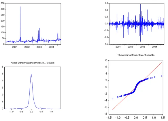
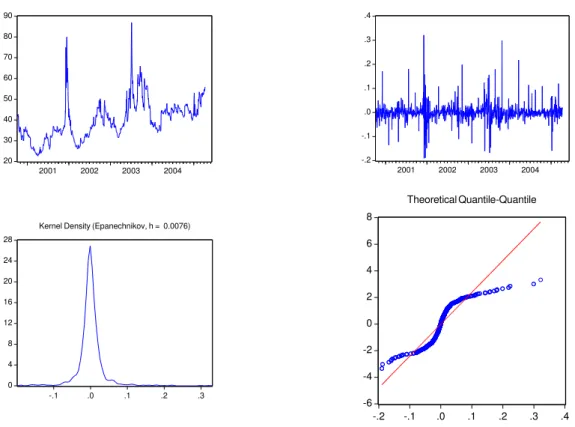
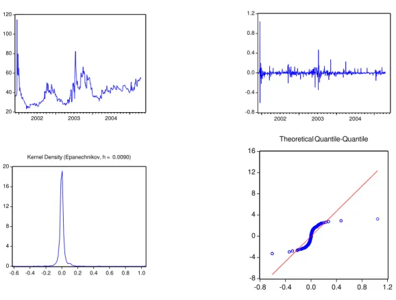
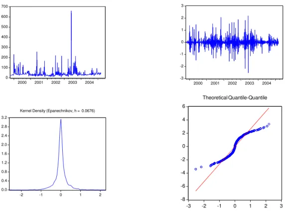
For each series of spot or forward prices, raw data Ptare converted to continuously compounded rates
of return yt ≡ ln(Pt/Pt−1). We then provide four figures for each series, namely the representation
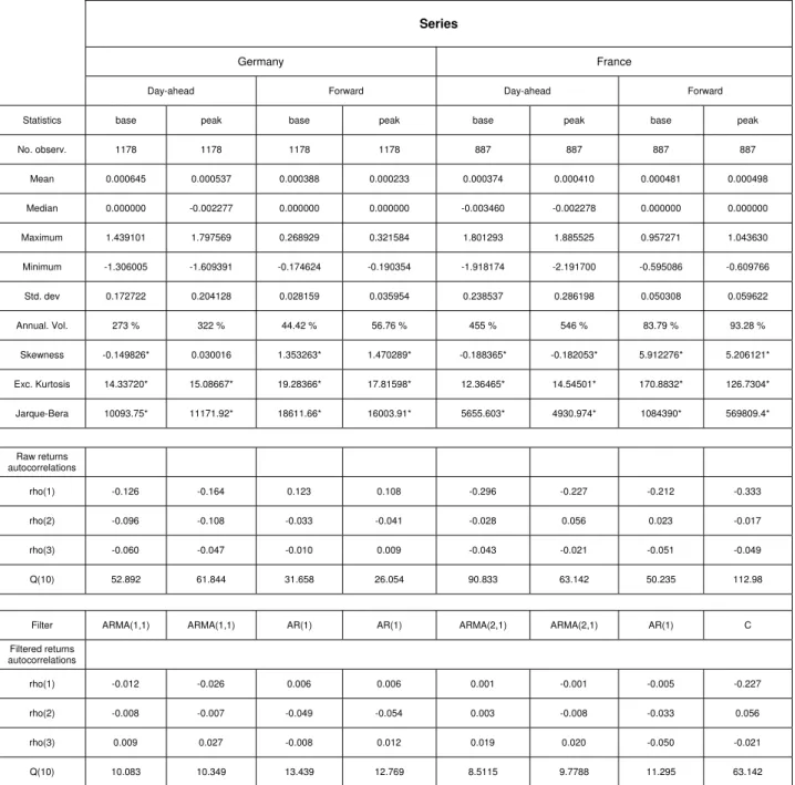
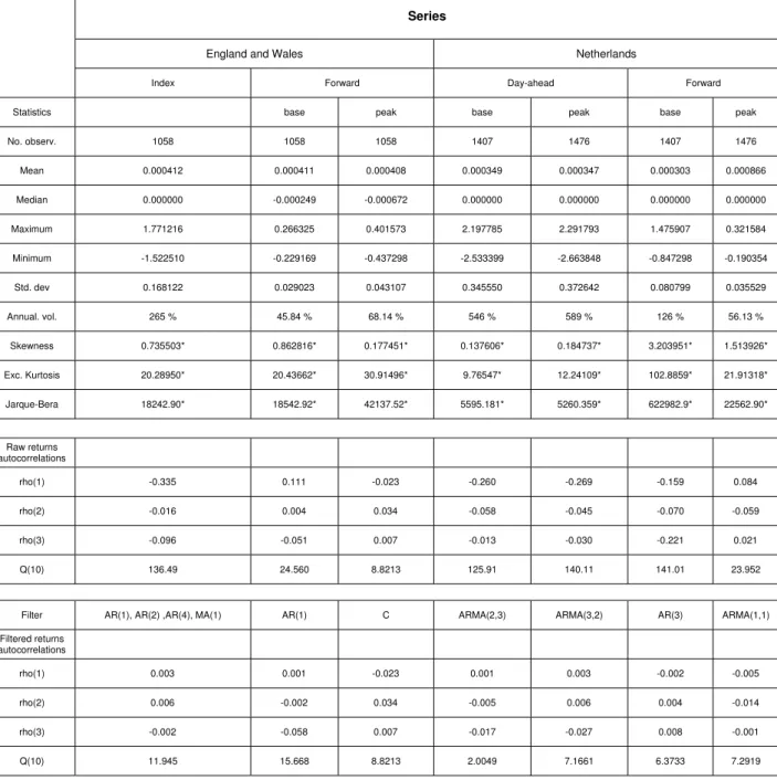
of raw data, return data, the kernel density of return data and a quantile-quantile plot (QQ-plot) against the Gaussian distribution. Simple observation of figures 1 to 15 confirms: (i) a very high level of volatility and the presence of some outliers in each series, (ii) an alternance of tranquil and volatil periods in return series (as described by Mandelbrot (1963) and Fama (1965)), (iii) an asymmetric distribution in most of the return series and (iv) a strong departure from normality. A wide range of descriptive statistics for returns are reported in tables 2 and 3. Inspection of the table reveals a mean return which is never significantly different from zero. The annualized volatility defined as √250 or √
365 times daily volatility, depending on the number of observations in a year, ranges from 44.42% to 126% for forward returns and from 265% to 589% for day-ahead returns. This exceptional level for volatility is a striking feature of power markets. Note that these levels of volatility far exceed figures provided in section 2.2 for other financial markets but are in line with historical volatilities in the U.S. markets.19
For all series, except day-ahead France and Germany, we observe a significant positive skewness, which confirms Bessembinder and Lemmon’s (2002) predictions. Because of the high level of sample-estimated skewness, the asymmetric behavior of the distribution may not be captured with a normal density. The observed kurtosis far exceed previous measures in other financial data, including com-modities returns and even emerging markets returns (see for instance Rockinger and Urga, 2001). This indicate the presence of many extreme returns implying thicker tails than normal in the distribution. Finally, the Jarque and Bera’s (1980) test is used to test for non-normality in the returns series. This test has only recently been shown to be valid for GARCH-generated processes by Fiorentini, Sentana and Calzolari (2004). The JB test strongly reject the normality hypothesis at any significance level, arguing for an alternative distribution. The need for a fat-tailed, possibly non-symmetric distribution
17During this study, we will call this trader “TRADER” (pseudonym) because the use of the data is subject to a
non-disclosure agreement.
18Heren, Platts, Argus or Bloomberg are major providers of OTC prices data for European energy markets. Note that
these information sources are extremely costly for academic purpose.
19Information gathered with professionals in electricity trading seems to indicate that differences observed in volatility
is then suggested.
We now concentrate on autocorrelations. As indicated by computed autocorrelations for the first three orders, our return data often exhibit some significant autocorrelation, suggesting a non random walk model as an appropriate filtration.20 This is confirmed with the Ljung-Box test statistics calculated at
the 10th order. In all cases (except French and British forward peak returns) the statistic indicate the presence of serial correlation. The extreme degree of kurtosis may however affect the power of the test. Autocorrelation is also present in emerging market return data, whose significant autocorrelation is generally related to thin trading and high transaction costs. The same applies for electricity markets. The presence of tranquil and more volatil periods is also confirmed through the use of Ljung-Box tests on squared returns, whose results are not reported here.21
4
Univariate analysis
Preliminary analysis suggested some ARMA-GARCH structures for our return series. Before multi-variate estimation, we determine the appropriate specification for each series, which will be kept in the multivariate case. The best lag structure for conditional means and variances are determined in the light of Akaike’s information criterion, Schwarz’ information criterion and residual diagnostic checks.
4.1
Econometric approach and estimation
After some filtration of the ARMA form for the return series – see tables 2 and 3 for the selected conditional mean equation specification – whose results are not reported here for sake of space, we search for the most appropriate GARCH(p, q) model for the parametrization of the conditional variance σ2 t as: σ2t = ω + p X i=1 βiσt−i2 + q X j=1 αjη2t−j (3)
with ηtthe disturbance term from the mean equation estimation or:
yt= E(yt|ψt−1) + ηt and ηt|ψt−1∼ D(ηt|ψt−1) (4)
where ψt−1denotes the σ-algebra generated by all the available information up through time t − 1 and
D(.|ψt−1) is an ad hoc distribution. As is well known, such a specification on the conditional variance
of rates of return allows for the alternance of more or less volatil periods as observed in Figures 1 to 15 and confirmed by some preliminary tests on the square of the residuals. The estimation is performed using the standard log-likelihood minimization. As demonstrated by Nelson and Cao (1992) The log-likelihood function for GARCH estimation needs not to be constrained.
4.2
Empirical results
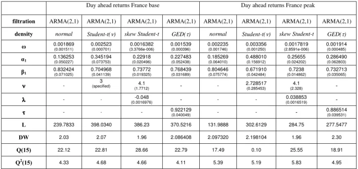
Tables 4 to 7 reports estimated parameters for the univariate GARCH specifications. In all cases but the German day-ahead base returns, we retain a GARCH(1,1) parametrization. This specification allows to remove any remaining serial correlation except for the German day-ahead peak returns.22
20Note that some autocorrelations in the returns are generally perceived as a proof of non efficiency in weak sense. Campbell
et al. (1997) note that serial correlation can exist in a long run General Equilibrium model without contradiction with the weak informational efficiency.
21Preliminary tests on the square of returns are not reported here as diagnostic tests. They are only used in a second step
to inspect for any remaining ARCH effect in the residuals.
Significance of parameters indicate that ARCH and GARCH effects exist in spot and forward returns series as suggested by returns plots in figures 1 to 15. In some cases, sums of coefficients are close to 1, indicating an integrated process. These results confirm previous results on electricity prices that persistence of volatility is strong (see for instance Hadsell et al. (2004)).
For all series, we perform TARCH or EGARCH specifications in order to detect any asymmetric responses to innovations.23 This kind of asymmetries is generally rejected in currency markets but
present in some stock and bond markets as well as in commodity markets. Our results indicate that there is no asymmetry.
4.3
Estimation under non-normality
A stylized fact of electricity return confirmed in our data is non-normality. GARCH models can take this feature into account. Indeed, despite the variability of the variance does not affect the unconditional variance, it does affect higher moments of the unconditional distribution of shocks. As shown in Campbell, Lo and MacKinlay (1997, p. 480), under heteroscedasticity, the unconditional distribution of the shocks has fatter tails than a normal distribution. Nevertheless, because of the strong non-normality of the financial returns, fitting of the conditional heteroscedastic models may still be enhanced by assuming a non-normal density for the error term.24 The very strong non normality
of our data also suggests to resort to non Gaussian densities.
Some papers assume a non-normal but symmetric distribution. Bollerslev (1987) uses a Student-t distribution to model the behavior of two exchange rates and five price indices. His GARCH(1,1)-t model fits the data better than a normal GARCH(1,1), which does not succeed in fully capturing the leptokurtosis aspect of the residuals. Baillie and Bollerslev (1989) compare Student-t distribution with exponential-power distribution in the study of exchange rates. Jorion (1988) selects a normal-Poisson mixture to model weekly exchange-rates. Nelson (1991) uses a generalized error distribution (GED). Hsieh (1989) uses Student-t, normal-lognormal mixture25, and GED (following Nelson (1991)) for the
modelling of daily exchange rates.
Other papers considers the issue of asymmetry. Hansen (1994) considers all moments as conditional. Theodossiou (1998) proposes an extension of the generalized Student-t distribution. The skewed GT distribution nests some other well-known probability distributions for some specific choice of the pa-rameters. A good survey on the use of non Gaussian densities – and particularly asymmetric densities – in conditionally heteroscedastic models is Bond (2000). The author emphasizes the asymmetric aspect of financial return series and the their treatment in the literature.
We retain four alternative distributions: the normal, the t, the Hansen’s (1994) skew Student-t and Student-the GED. Log-likelihood funcStudent-tions for Student-these densiStudent-ties are wriStudent-tStudent-ten using Student-the expression of Student-the density functions. For the Student-t density with ν degrees of liberty it is:
g(x|ν) = Γ ³ ν+1 2 ´ p π(ν − 2)Γ ³ ν 2 ´³1 + x 2 (ν − 2) ´(ν+1)/2 (5)
23The asymmetric response models allow to consider the so-called “leverage effect” highlighted by Black (1976). Despite
the possible existence of nonlinear dynamics in electricity returns, we do not use the APARCH model by Ding et al. (1993) which requires nonlinear optimization techniques (see Giot et Laurent (2003) for more details and an application to the determination of VaR bounds for several commodities).
24Bollerslev (1987, p. 544): “Even though the unconditional distribution corresponding to the GARCH(p, q) model
with conditionally normal errors is leptokurtic, it is not clear whether the model sufficiently accounts for the observed leptokurtosis in financial time series.”
The skewed Student-t density with ν degrees of liberty and an asymmetry parameter λ is written: g(x|ν, λ) = bc ³ 1 + 1 ν−2 ³ bx+a 1−λ ´2´−(ν+1)/2 x < −a/b bc ³ 1 + 1 ν−2 ³ bx+a 1+λ ´2´−(ν+1)/2 x ≥ −a/b (6)
with 2 < ν < ∞ and −1 < λ < 1 and the constants a,b and c as follows:
a = 4λc³ ν − 2 ν − 1 ´ ; b2= 1 + 3λ2− a2 ; c = Γ ³ ν+1 2 ´ p π(ν − 2)Γ ³ ν 2 ´ (7)
And the GED density is:
g(x|ν) = νΓ ³ 3 ν ´ 23 r Γ ³ 1 ν ´ exp(−12 ¯ ¯ ¯x λ ¯ ¯ ¯ν) (8)
where λ = Γ(1/ν)1/2Γ(3/ν)−1/22−2/ν is used to normalize the variance.
Tables 4 and 5 illustrate the better goodness of fit of non Gaussian distributions for French returns. The log-likelihood is always improved. This highlights the need for leptokurtic distribution for power returns data. However it is not possible to compare improvements for day-ahead and forward series. Note that results are similar for series of other countries.
5
Multivariate analysis and optimal hedging
As argued in the introduction, multivariate models can be used for the computation of optimal hedge ratios. Selected multivariate models for our study are: the BEKK model, the CCC model and the DCC model.26
5.1
Multivariate GARCH: the general case
The general specification for a constant correlation multivariate GARCH model of a n-dimensional process yt= (y1,t, ..., yn,t)0 is given by:
yt= E[yt|Ψt−1] + ηt (9)
ηt= ztΣ1/2t with E(zt) = 0 ; Vart(zt) = In (10)
where E[.|Ψt−1] is the expectation operator conditionally to the available information on all series.
ηt= (η1,t, ..., ηn,t)0 is the vector of innovations and Σt≡ [σij,t] is a n × n positive definite matrix with
σij,t= Covt(ηi,t+1, ηj,t+1). Because σii,t= Vart(ηi,t+1), Σ1/2t is a positive definite matrix. From these
properties of z and (10), it follows that E[ηη0|Ψ
t−1] = Σt. We then have a vector of returns whose
covariance matrix evolves through time. The mean equation (9) can be thought as a filtration for non zero mean returns.
26Recent surveys on MGARCH models are Bauwens, Laurent and Rombouts (2006) and Silvennoinen and Ter¨asvirta
In its most general form, the parametrization for the conditional covariance matrix was proposed by Bollerslev, Engle and Wooldridge (1988) as27:
vech(Σt) = ω + Φvech(Σt−1) + Λvech(ηtη0t) (11)
This general parametrization model Σt as a linear function of lagged values of Σt, lagged squared
errors and cross products of errors. The “curse of dimensionality” arises in this model because of the number of parameters to estimate in this model, which is O(n4), precisely n2(n + 1)2/2 + n(n + 1)/2.
In the case of three series, the number of parameters to estimate is for instance 78. In order to keep the model manageable for more than two series, restrictions have to be placed on this specification. In this respect, Bollerslev et al. (1988) assume Φ and Λ diagonal. In this VEC model, Σt only
depends in a linear way on its own lagged values and on lagged square errors. In this simpler model, the number of parameter to estimate becomes 3n(n + 1)/2 and thus only grows as O(n2).
To maintain a reasonable number of parameters and positive definiteness of the covariance matrix, different parametrizations for the conditional covariances matrices are proposed.
5.2
The BEKK model
We first study the BEKK model of Engle and Kroner (1995) (named after an earlier working paper by Baba, Engle, Kraft and Kroner). In its full parametrization, the BEKK model can be written as:
Σt= C0C + B0Σt−1B + A0ηt−1ηt−10A (12)
where C is a lower triangular matrix, and B and A are square matrices. Positive definiteness is guaranteed by the use of quadratic forms. Hence, strong restrictions that have to be made on the VEC model to ensure positive definiteness are bypassed. Restrictions of the BEKK model include the diagonal BEKK and the scalar BEKK. In the diagonal BEKK, matrices B and A are diagonal matrices. In the scalar BEKK, B and A are scalars. The richness of the structure is then greatly reduced and refers to the VEC model.
Drawbacks from the BEKK parametrization are: (i) the remaining significant number of parameters to estimate which still grows with O(n2). For a BEKK model with one lag on ARCH and GARCH
components, this give (5n2+ n)/2 coefficients (24 parameters for a trivariate BEKK(1,1,1) model).
(ii) the impossibility to interpret estimated coefficients. Any covariability persistence is then difficult to characterize. (iii) the implicit hypothesis of a constant correlation structure. It is then useful to enrich the structure of the model by allowing for time-varying correlations.
5.3
The Bollerslev’s (1990) CCC
In the Bollerslev’s (1990) model, covariances between i and j are allowed to vary only through the product of standard deviations with a correlation coefficient which is constant through time. The dynamic of standard deviations is governed by the GARCH(1,1) variances’ dynamic or any univariate GARCH model. Keeping the covariance matrix Σt≡ [σij,t], we have:
σii,t= ωii+ βiiσii,t−1+ αiiη2i,t (13)
and
σij,t= ρij√σii,tσjj,t (14)
27The “vech” (half - vec) operator stacks the non-redundant elements of a matrix – those on and below the main diagonal
As pointed out by Bollerslev (1990), under the assumption of constant correlation, MLE of the corre-lation matrix and sample-based correcorre-lation matrix coincide. Because of the positive semi-definiteness of the sample-based estimate, the same is guaranteed for the conditional covariance matrix. The main advantage of this model is to greatly simplify computation by keeping out of the likelihood function the correlation matrix. The number of parameters to estimate when a GARCH(1,1) is retained is n(n + 5)/2. The main drawback of this model is that the sign of the conditional correlation is constant over time once ρij is estimated. This may be a problem in the estimation of OHRs. This model has
been use, without success, for hedging purpose in Lien, Tse and Tsui (2002) on a panel of financial and non financial commodities.
5.4
Testing for non constant correlation
Tests of constant correlation have been proposed by Tse (2000) and Bera and Kim (2002). Details about these tests are given in the appendix. The use of these two tests is interesting for our data because while the IM test has good approximate nominal size, it lacks power. Empirical illustrations show that the constant correlation hypothesis is sometime severely rejected only because of the non-normality of the data. Conversely, the LM test is less adapted for smaller samples but is relatively robust against non-normality. Consequently, both tests are complements in our analysis.
Computed statistics for our data do not indicate any strong rejection or acceptance of the null hypoth-esis of constant correlation. For instance for France, the LMC – which follows a χ2with one degree of
freedom under the null of constant correlation – is 7.81.10−4 rejecting the hypothesis of non constant
correlation.28 Conversely, the value of the IM test we compute is 5.37 (with same critical levels). The
IM test thus argues for a rejection of the constant correlation hypothesis. We also perform a studen-tized version of the test. The value obtained is 0.250 arguing for a rejection of the null hypothesis. These findings are identical for other series and we then decide to estimate the DCC model for all series in order to investigate further the correlation constancy.
5.5
The DCC model of Engle (2002)
As highlighted by Erb, Harvey and Viskanta (1994), Longin and Solnik (1995,2001) or Tsui and Yu (1999), correlations between returns may not be constant in time. In their studies, correlations are stronger when prices are falling. To model this feature of the series some dynamic correlation models can be employed in order to avoid an implicit loss of information when estimating conditional variances and covariances. Among dynamic correlation models are Christodoulakis and Satchell (2002), Tse and Tsui (2002) and Engle (2002). We retain the Engle’s model for its tractability.
The general form of the Dynamic Conditional Correlation model introduced by Engle (2002) and Engle and Sheppard (2001) is defined by:
Σt≡ DtRtDt (15)
Rt≡ Q∗−1t QtQ∗−1t (16)
Qt= (1 − P X p=1 αp− Q X q=1 βq)Q + P X p=1 αp(ηt−pηt−p0) + Q X q=1 βqQt−q (17)
where Dt is a n × n diagonal matrix of time varying standard deviations defined by any univariate
GARCH model, Dt is a n × n time varying correlation matrix, Qt is defined by (16), Q is the
unconditional covariance matrix using standardized residuals from the univariate estimates, and Q∗t is a diagonal matrix of the square root of the diagonal elements of Qt. We then have the time varying correlation matrix defined as Rt ≡ [ρij,t] with [ρij,t] = √qqij,tiiqjj. Engle and Sheppard (2001) give
sufficient conditions for the positive definiteness of the DCC model.
Interestingly, the DCC model can be estimated in two steps and the number of parameters to estimate is greatly reduced. The model is then manageable for a greater number of series. The model also keeps intuition in the interpretation of the parameters, which is lost by using a factor model in the spirit of Diebold and Nerlove (1989) where parameters describe an unobserved variable. Nevertheless, this simplification is made at a cost. Indeed, an implicit assumption of the DCC model is that αp and
βq being scalars, all correlations obey the same dynamic.
5.6
Estimation results
The number of estimated parameters for the BEKK model is high and have no direct interpretation, so we do not report estimates here. For each series, all coefficients are significant, indicating that covariance matrix is dependent from its lagged value and dependent from lagged innovations. Despite the fact that the model seems to be well specified, the variance reduction is near zero or even negative (see Table 9). This conclusion confirms the poor power of the BEKK model for hedging purpose as highlighted by Bera et al. (1997) among others. This also questions the deeper issue of the predictive power of conditionally autoregressive heteroscedastic models. In addition, the computed OHRs with the BEKK specification appear highly volatil (see figure 16 for the French case) but ratios are similar in magnitude to Moulton’s (2005) hedge ratios.29 Estimation of the CCC model give identical results
with no variance reduction despite significant estimated parameters. This confirms findings from Lien et al. (2002) about low hedging effectiveness of the CCC model.
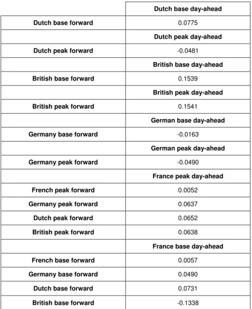
Estimation results for the DCC model are only reported for French data (see table 10). Again, results for other countries are in line with the French case. We observe that coefficients γ and δ are near from zero, indicating the absence of a dynamic structure for correlation. This may confirm the Tse’s (2000) test whose results reject the hypothesis of non constant correlation. Optimal hedge ratio and variance reduction for this model is computed but, of course, no significant improvement appears. Maybe the expected improvement for hedge ratio forecasting through the use of a dynamic correlation model is not achieved because of the very low sample correlation coefficient in our data. Some further investigations with other financial data may help to conclude on the power of this model for correlation forecasting.
The estimated parameters for the DCC model are provided in Table 10. Again, the estimates are significant for the spot returns but the ARCH term is not for forward returns. However, the model does not improve the CCC specification and gives similar conditional moments and optimal hedge ratio.
6
Concluding remarks
The analysis of returns of spot and forward markets for France, Germany, the Netherlands, and the UK leads us to conclude to a strong rejection of the random walk hypothesis. For all the series (except French and British forward peak returns) an autoregressive, possibly moving average, specification has to be retained. However, the use of non Gaussian densities greatly improves the data fit, particularly for spot returns. After filtration, a GARCH behavior is identified for all series, indicating a memory in the evolution of the returns’ variance.
As suggested by the very low level of sample correlations, the hedging effectiveness of forward markets is insignificant, especially if transaction costs are considered. More sophisticated time series techniques than the conventional OLS computation for the OHR do not improve – and sometimes decrease – variance reduction. Determination of the OHR through the use of dynamic correlation model does not enhance our results.
The present study can be extended in a number of directions. First, power of dynamic conditional correlation models may be further investigated using less specific financial data. Second, hedging effectiveness of European forward markets may be analyzed with other hedging horizons. Third a hedging portfolio in the spirit of Gagnon et al. (1998) may be computed, but we definitely doubt of the potential of forward markets for hedging purpose, at least for short-term. Fourth, the paper strongly argue in favor of non normal densities and this line of research, particularly active nowadays (see for instance Bauwens and Laurent (2005)), is promising for electricity returns. Finally, the specification of higher moments transmission and/or models of volatility transmission (see Hansen (1994), Harvey and Siddique (1999) and Brooks et al. (2005)) may provide interesting insights about the European integration of the electricity industry.
Appendix: testing for constant correlation in a MGARCH
Tse’s (2000) Lagrange Multiplier test
To test the relevancy of any dynamic model, we first use the Lagrange Multiplier (LM) test by Tse (2000). We do not retain the test suggested by Bollerslev (1990) because it is inappropriate as pointed out by Li and Mak (1994).30 In addition, Bollerslev’s procedure is not a test for constancy of correlation but for linear dependence between the conditional correlation coefficient ant its lagged values. Interestingly, Tse’s test does not need to estimate an encompassing model. The constant-correlation model is extended in way that allows for time-varying correlations and some key parameters in this extended model are then imposed to be zero. Study of the properties of the test in small samples using Monte Carlo methods shows that it has good approximation nominal size in sample sizes of 1000 or above.
Tse considers the following specification for the time-varying correlations:
ρij,t= ρij+ δijηi,t−1ηj,t−1 (18)
The constant correlation hypothesis can then be tested by examining the hypothesis H0: δij= 0 for all i and j. Nevertheless, specification in equation (18) does not guarantee that ρij,t is always below 1. This issue is left for the optimization stage.
The conditional variance matrix is defined as in the CCC original model and allows to compute the log likelihood Ltfor t = 1, ..., T in order to estimate the k parameters. We then obtain the k × 1 vector of scores s = ∂L/∂θ). We denote S as the T × k matrix with rows as score vectors defined above. The proposed LMC
statistic to test H0 is:
LM C = ˆs0( ˆS0S)ˆ−1ˆs = l0S( ˆˆ S0S) ˆˆS0l (19) with l the T × 1 column vector of ones and ˆS is S evaluated at ˆθ. The statistic is asymptotically distributed
as a χ2
M with M = n(n − 1)/2 the number of additional restrictions placed to constrain the model.
Bera and Kim’s (2002) Information Matrix test
A second test is Bera and Kim (2002). Their test is based on the Chesher’s (1984) interpretation that White’s information matrix (IM) test is a test of parameter heterogeneity. They thus apply this test to the Bollerslev’s (1990) CCC model to test for the constancy of parameters in time.
The test is based on the hypothesis that the variances of the parameters of interest are zero assuming they are constant through time. The test is not based on an arbitrary distributional assumption despite it is shown to be rather sensitive to non-normality. In addition, unlike Longin and Solnik (1995) and Tse (2000), absolute value of the correlation coefficient has no risk to exceed 1. The proposed statistic is derived from the efficient score form of the IM matrix test proposed by Orme (1990) and takes the form:
IMe= h PT t=1(ˆv ∗2 1tvˆ2t∗2− 1 − 2ˆρ2) i 4T (1 + 4ˆρ2+ ˆρ4) (20) with ˆ ρ = 1 T T X t=1 ˆ η∗ 1tηˆ2t∗ (21) and ˆ v∗ t = (ˆv∗1t, ˆv2t∗)0= ³ η∗ 1t− ρη2t∗ p 1 − ρ2 , η∗ 2t− ρη∗1t p 1 − ρ2 ´0 (22) where η∗
1t and η∗2t are standardized residuals for series 1 and 2, respectively. Under the null hypothesis of constant correlation, IMe follows a χ2 with one degree of freedom. Monte Carlo simulations show that the
behavior of the test is not too bad using a Student-t distribution.
30The Ljung-Box portmanteau test suggested by Bollerslev uses cross products of the standardized residuals and critical
values are based on the χ2 distribution. However the portmanteau statistic is not asymptotically distributed as a χ2
References
Alexander, C., Chibumba, A., 1997. Multivariate orthogonal factor GARCH. University of Sussex, Mimeo.
Allaz, B., Vila, J.-L., 1993. Cournot competition, forward markets and efficiency. Journal of Economic Theory 59, 1-16. Baillie, R., Bollerslev, T., 1989. The message in daily exchange rates: a conditional variance tale. Journal of Business
and Economic Statistics 7, 297-305.
Baillie, R.T., Myers, R.J., 1991. Bivariate GARCH estimation of the optimal commodity futures hedge. Journal of
Applied Econometrics 6, 109-124.
Barlow, M.T., 2002. A diffusion model for electricity prices. Mathematical Finance 12, 287-298.
Bauwens, L., Laurent, S., 2005. A new class of multivariate densities, with application to GARCH models. Journal of
Business and Economic Statistics 23, 346-354.
Bauwens, L., Laurent, S., Rombouts, J.V.K., 2006. Multivariate GARCH models: a survey. Journal of Applied
Econo-metrics 21, 79-109.
Bera, A.K., Garcia, P., Roh, J., 1997. Estimation of time-varying hedge ratios for corn and soybean: BGARCH and random coefficient approaches. Sankhya 59, 346-368.
Bera, A.K., Kim, S., 2002. Testing constancy of correlation and other specifications of the BGARCH model with an application to international equity returns. Journal of Empirical Finance 2002, 171-195.
Bessembinder, H., Lemmon, M.L., 2002. Equilibrium pricing and optimal hedging in electricity forward markets. Journal
of Finance 2002, 1347-1382.
Black, F., 1976. Studies of stock market volatility changes. 1976 Proceedings of the American Statistical Association,
Business and Economic Statistics Section, 177-181.
Boisseleau, F., 2004. The role of power exchanges for the creation of a single European electricity market: market design
and market regulation. PhD dissertation, Delft University.
Bollerslev, T., 1987. A conditionally heteroskedastic time series model for speculative prices and rates of return. Review
of Economics and Statistics 69, 542-547.
Bollerslev, T., 1990. Modelling the coherence in short-run nominal exchange rates: a multivariate generalized ARCH approach. Review of Economics and Statistics 72, 498-505.
Bollerslev, T., Engle, R.F., Wooldridge, J.M., 1988. A capital asset pricing model with time varying covariances.
Journal of Political Economy 96, 116-131.
Bollerslev, T., Wooldridge, J.M., 1992. Quasi-maximum likelihood estimation and inference in dynamic models with time varying covariances. Econometric Reviews 11, 143-172.
Bond, S.A., 2000. A review of conditional density functions in autoregressive conditional heteroscedasticity models. In: Knight, J. and Satchell, S.E. (eds) Return Distributions in Finance, Butterworth and Heinemann, Oxford.
Bosco, B., Parisio, L., Pelagatti, M., Baldi, F., 2006. Deregulated wholesale electricity prices in Europe. Mimeo, Universit`a Milano-Bicocca.
Bower, J., 2002. Seeking the single European electricity market – Evidence from an empirical analysis of wholesale market prices. Working Paper EL01, Oxford Institute for Energy Studies.
Brooks, C., Burke, S.P., Heravi, S., Persand, G., 2005. Autoregressive conditional kurtosis. Journal of Financial
Econometrics 3, 399-421.
Bystr¨om, H.N.E., 2003. The hedging performance of electricity futures on the Nordic power exchange. Applied Economics 35, 1-11.
Bystr¨om, H.N.E., 2005. Extreme value theory and extremely large electricity price changes. International Review of
Economics and Finance 14, 41-55.
Campbell, J.Y., Lo, A.W., MacKinlay, A.C., 1997. The Econometrics of Financial Markets. Princeton University Press, Princeton, NJ.
Cecchetti, S.G., Cumby, R.E., Figlewski, S., 1988. Estimation of the optimal futures hedge. Review of Economics and
Statistics 70, 623-630.
Christodoulakis, G.A., Satchell, S.E., 2002. Correlated ARCH: modelling the time-varying correlation between financial asset returns. European Journal of Operational Research 139, 351-370.
Christodoulakis, G.A., 2007. Common volatility and correlation clustering in asset returns. European Journal of
Opera-tional Research, in press.
De Vany, A.S., Walls, W.D., 1999. Cointegration analysis of spot electricity prices: insights on transmission efficiency in the western US. Energy Economics 21, 435-448.
Ding, Z., Granger, C.W.J., Engle, R.F., 1993. A long memory property of stock market returns and a new model.
Journal of Empirical Finance 1, 83-106.