Model checking of steady-state rewards using
bounding aggregations
Hind Castel
GET/INT/SAMOVARINT
9,rue Charles Fourier 91011 Evry Cedex, France
Lynda Mokdad
Lamsade Laboratory Universit´e de Paris Dauphine Place du Mar´echal de Lattre de Tassigny75775 cedex 16, France [email protected]
Nihal Pekergin
LACL Laboratory Universit´e Paris Est 61, av. du G´en´eral de Gaulle 94010 Cr´eteil Cedex, France [email protected]Abstract—This paper presents an algorithm based on
stochas-tic comparisons in order to check formulas with rewards on multidimensional Continuous Time Markov Chains (CTMC). These formulas are expressed in Continuous Stochastic Logic (CSL) which includes means to express transient, steady-state and path performance measures. However, computation of transient and steady state distribution are limited to relatively small sizes because of the state space explosion problem.
We propose a model checking algorithm based on aggregated bounding Markov processes in order to perform the verification on the bounds values instead of the exact one. The stochastic comparison has been largely applied in performance evaluation however the state space is generally assumed to be totally ordered which induces less accurate bounds for multidimensional Markov processes. We use the increasing set theory and the comparison by mapping functions in order to derive bounds on reduced state spaces. The relevance of the proposed checking algorithm is the possibility of a parametric aggregation scheme in order to improve the accuracy of the bounds and in the same time the precision of the checking, but in return with an increasing of the complexity.
I. INTRODUCTION
Continuous Time Markov Chain (CTMC) is the most use-ful mathematical model underlying many formalisms for the description and the quantitative analysis of stochastic discrete-event dynamic systems. Once a CTMC has been generated, the next step is to compute performance measures such as throughput, loss probabilities, etc. Continuous Stochastic Logic CSL can be used to express constraints on such mea-sures and model checking techniques are applied to automated analysis of these constraints. The CSL [1] was developed as a stochastic extension of the branching-time Temporal Logic (CTL) [5]. Stochastic model checking has been extended to models with some rewards on states and transitions in which logic formalisms as Probabilistic Reward Computational Tree Logics (PRCTL) and Stochastic Reward Logic (CSRL) [9] are used for performance and dependability applications.
We propose to check the rewards based formulas of stochas-tic models by applying stochasstochas-tic comparison approach. To check these formulas, transient or steady-state distribution of underling Markov chain must be computed. However, these models are usually represented by multidimensional processes
with very large state spaces. As a result, quantitative analysis to check formulas, is difficult if there is no specific solution form (product form solutions, ...). Since exact performance measures can only be obtained using numerical methods [18] with small sizes, it is important to develop new powerful mathematical tools for large state systems.
Related works. In this paper, we propose a model checking
algorithm in order to verify reward formulas on aggregated bounding Continuous Time Markov Chain (CTMC). In [15], a stochastic comparison based method is proposed to check state formulas defined over Discrete Time Markov Chain (DTMC) rewards. The authors have assumed a total order, and generate the aggregated Markov chains using the LIMSUB algorithm [8], based on lumpability constraints. In the present paper, we use an algorithm generating bounding aggregated Markov chains presented in [3], [4]. It is based only on a partial order which induces less constraints then a total order, and so more accurate bounds for multidimensional Markov processes. Also, we propose a parametric aggregation scheme in order to improve the accuracy of bounds and also the precision of the checking.
In [1,17], model checking algorithms for CTMC are pro-posed using lumping equivalence in order to reduce Markov chains state spaces. The notion of state equivalence relation also called stochastic bisimulation is introduced in order to build a reduced state space called quotient. The relation is based on the required conditions that must have equivalent states as equality of state labelling, rewards, exit rates. The advantage is the verification of CSL logic formulas on a reduced state space.
Compared with this study, the algorithm which we propose does not suppose lumping equivalence, and so it is easier to aggregate the state space, but in return the verification is made on bounding values instead of exact ones which does not let to decide for all cases.
This paper is organized as follows. Next, we present the CSL logic, focusing on formulas with rewards for perfor-mance study. In the section after, we present the stochastic comparison method on multidimensional state spaces in order
to generate aggregated bounding Markov chains. In section IV, we apply the algorithm to the model checking of large state Markov chains. We use the increasing set theory in order to generate bounds on performance measures with rewards. The section V is devoted to checking if loss probabilities in a tandem queueing network is included or not in an interval. Different parametric aggregation schemes have been proposed in order to show the trade off between improving the precision of the checking, and increasing the state space. As a conclusion, we resume advantages and limits of our approach. Finally, we resume in an appendix the stochastic ordering theory used in this paper.
II. MODEL CHECKINGMARKOV CHAINS
Continuous Stochastic Logic (CSL) is an extension of Computation Tree Logic (CTL) with two probabilistic oper-ators that refer to steady-state and transient behaviors of the underlying system.
CSL is a branching-time temporal logic with state and path formulas. The states formulas are interpreted over states of a CTMC, whereas the path formulas are interpreted over paths in CTMC [1]. In order to express the time span of a certain path, the path operators until (U) and next (X ) are extended with a parameter that specifies a time interval [1].
The CSL logic has been extended to continuous stochastic reward logic (CSRL) to specify performability measures over Markov reward models (MRMs). It contains operators that refer to the stationary and transient behaviour of the considered systems. To specify performability measures as logical formu-las over MRMs, it is assumed that each state is labelled with so-called atomic propositions. Atomic propositions identify specific situations the system may be in, such as “buffer full“, “buffer empty“ or “variable X is positive“ [9].
The MRM is a tuple M = (E, R, ρ) where E is a finite set of states, R : E × E −→ R≥0 is the rate matrix, and
ρ : E −→ R≥0 is a reward structure that assigns to each state
s a reward ρ(s), also called cost. The MRM has a fixed initial distribution α satisfying !s∈Eαs= 1, so the MRM starts in
state s with probability αs.
CSRL allows one to specify properties over states and over paths. A path is an alternating sequence s0t0s1t1. . . where
si is a state of the MRM and ti > 0 is the sojourn time in
state si. The accumulated reward for a finite path of length
n is given by !ni=0−1tiρ(i). Let I and J be intervals on the
real line, p a probability and #, a comparison operator, such as > or <. The syntax of CSRL is defined by the following grammar [9]: State-formulas: φ ::= true| a | φ ∨ φ | φ ∧ φ | ¬φ | P!p(φ) Path-formulas: φ ::= (φUI Jφ)| XJI(φ)
For the state formulas¬, ∨ and ∧ the meanings are as usual. For the formulaP!p(φ), it is valid in state s if the probability
measure of the set of paths starting in s and satisfying path
formula φ meets the bound #p. The path-operators nextX and untilU are used with two intervals. Interval I can be considered as a timing constraint whereas J represents a bound for the cumulative reward. In the following, we give examples for the both path-operators.
• P≤0.2(X(0,≤5∞)s) which means that with a probability at
most 0.2, a transition can be made to s-states at time t∈ [0, 5] such that the accumulated reward until t lies in (0, ∞).
• P≤0.2(aU(0,∞)≤5 b)) which means that b-state can be
reached with probability at least 0.2 at time t ∈ [0, 5] along a-states such that the accumulated reward until t lies in (0,∞).
In this paper, we consider steady-state reward formulas as given in [1] for discrete time Markov chains:
Steady-state Reward-formulas:
εI(φ) | L!p(φ)
These formulas are inspired from performance measures of CTMC with rewards.
• The formula εI(φ) is the long-run expected reward for
φ-states. If the steady-state exists, εI(φ) is satisfied if:
εI(φ) is satisfied iff
"
s!|=φ
π(s&)ρ(s&) ∈ I
• The formula L!p(φ) asserts that the steady state
proba-bility to be in φ-states meets the bound #p. L!p(φ) is satisfied iff
"
s!|=φ
π(s&) # p III. STOCHASTIC COMPARISON OF MULTIDIMENSIONAL
MARKOV PROCESSES
The stochastic comparison is a mathematical tool which allows to compute bounds on transient distributions and the stationary distribution of a Markov process. In fact, if the un-derlying Markov process does not have a specific solution form like a product-form or matrix-geometric solutions, etc. the computation of stationary probability distributions becomes difficult or intractable for multidimensional large state spaces. By means of the stochastic comparison method, it is pos-sible to overcome this problem by reducing the size of the state space of the underlying Markov process. Stochastic comparison is based on the definition of stochastic orderings between random variables, probability measures, or stochastic processes. In this paper, we use the stochastic comparison by mapping functions in order to reduce the state space size. We have summarized in the appendix the main concepts of stochastic comparisons of multidimensional Markov processes used in this paper.
Let X(t) be a large state space Markov process defined on a multidimensional and preordered (not necessarily a totally ordered) state space E, with an infinitesimal generator matrix Q. We suppose that the process is irreducible so the stationary
distribution Π exists, but it is very difficult to compute (not a specific solution form, and a large state space size).
The study of this system consists in the checking of the formula εI(φ), which is true if :
R(φ)∈ I where :
R(φ) ="
s|=φ
Π(s)ρ(s)
so εI(φ) is satisfied if the long-run expected reward rate per
time-unit for φ-states meets the bound of I = [Imin, Imax]. If
there is a closed-form for Π then it will be easy to compute and the verification can be easiliy done . Otherwise, as the state space size increases exponentially with the number of components, then it will be very difficult to verify εI(φ).
We propose to define aggregated bounding Markov processes [3,4], in order to derive an aggregated upper (resp. lower) bounding Markov process, from which we can compute the stationary distribution Πu(resp. Πl) defined on a smaller state
space. We verify the formula εI(φ) by computing an upper
bound (resp. a lower bound) Ru(φ) ( resp. Rl(φ)) to R(φ),
and testing if they are included in I.
We use the algorithm generating aggregated bounding Markov processes [3]. The goal of the algorithm is to derive :
• The Markov process {Xu(t), t ≥ 0} representing the
upper bound computed from{X(t), t ≥ 0}, and the many to one mapping function gu: E → Su, Su⊂ E.
• The Markov process {Xl(t), t ≥ 0} representing the
lower bound, computed from {X(t), t ≥ 0}, and the mapping function gl: E → Sl, Sl
⊂ E.
In [3], we have proved using the stochastic ordering theory described in the appendix that the algorithm generates aggre-gated Markov processes bounds for the exact process. For the upper bound, we have the comparison by the mapping function gu :
{gu(X(t)), t ≥ 0} *st{Xu(t), t ≥ 0}
and for the lower bound, by the mapping function gl:
{Xl(t), t ≥ 0} *st{gl(X(t)), t ≥ 0}
As results of the comparison of the processes, we have the comparison of transient and stationary probability distribu-tions. Only the second one is used in this paper, it is explained in the next section.
A. Probability distributions comparison
We consider here only the stationary case. From the propo-sition 1 in the appendix, we have the following relations :
" x|gu(x)∈Γ Π[x]f(x) ≤" x∈Γ Πu[x]f(x), ∀Γ ∈ Φ st(Su) (1) and : " x∈Γ Πl[x]f(x) ≤ " x|gl(x)∈Γ Π[x]f(x)∀Γ ∈ Φst(Sl) (2)
where f : E→ R>0, is an increasing function.
IV. MODEL CHECKING ON AGGREGATED BOUNDING
CTMC
In this section we use the stochastic comparisons and pre-cisely the algorithm generating aggregated Markov processes in order to check steady-state reawrd formulas.
A. States formulas bounds
We focus on the state formula with rewards εI(φ), and we
want to verify if it is true or not. We need to compute R(φ) given by :
R(φ) = "
s∈Eyes
Π[s]ρ(s)
where Eyes = {s ∈ E|s |= φ}, and ρ : E → R>0 is
not necessary an increasing function. For multidimensional processes, it is difficult to compute Π if there is no product form, because the state space size increases exponentially. So we propose to compute bounds to R(φ) in order to verify εI(φ). These bounds are computed from aggregated bounding
Markov processes generated from the exact Markov pro-cess. We apply the algorithm generating aggregated bounding Markov processes [3] in order to derive bounding aggregated Markov processes.
As some states of Eyeswill be aggregated, then the
compu-tation of the bounds will be made on the states of gu(E yes) for
the upper bound, and gl(E
yes) for the lower bound. Although
Eyes is not an increasing set, we could have the aggregated
sets gu(E
yes) and gl(Eyes) defined as increasing sets. In
the example 1 of the appendix, Eyes = {(0, 1)} is not an
increasing set, but g(Eyes) = {(1, 1)} is an increasing set.
We suppose that gu(E
yes) and gl(Eyes) are increasing sets
which could be very useful for the stochastic comparison of the stationary distributions.
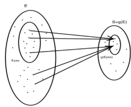
E Eyes . . .. .. . .. . .. . . . . . . . . . . . . . . . . . . . . S=g(E) g(Eyes) . . . .. . . . . .
Fig. 1. Aggregation of Eyes: the general case
From proposition 2 of the appendix, and Fig.1 where g is replaced by gu, we have : " x∈Eyes Π[x] ≤ " x|gu(x)∈gu(E yes) Π[x]
If we use the reward function ρ, and if we define an increasing function ρ1, representing an upper bound to ρ, then
we have the following inequality : R(φ) = "
x∈Eyes
ρ(x)Π[x]≤ "
x|gu(x)∈gu(Eyes)
ρ1(x)Π[x]
From equation 1 in section III-A , as gu(E
yes) is an
increasing set of Φst(Su), then we obtain :
" x|gu(x)∈gu(Eyes) ρ1(x)Π[x] ≤ Ru(φ) = " x∈gu(Eyes) ρ1(x)Πu[x] So we deduce that R(φ)≤ Ru(φ)
We study now the lower value case. From proposition 2 in the appendix, and figure Fig.1, where we replace g by gl, we
have : " x∈Eyes Π[x] ≤ " gl(x)∈gl(Eyes) Π[x]
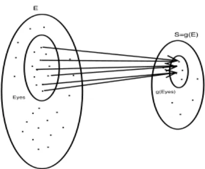
It is clear that the inequality sense is inadequate with the definition of a lower bound. We suppose the particular case where the states of gl(E
yes) are the mappings of states which
are only in Eyes, and not outside Eyes, as it is represented
in Fig.2. This assumption will be possible if we can define a mapping function gl from the set E
yes , verifying this
condition. E Eyes . . .. .. . .. . .. . . . . . . . . . . . . . . . . . . . . S=g(E) g(Eyes) . . . .. . . . . .
Fig. 2. Aggregation of Eyes: a particular case
It is equivalent to say that :
- ∃x | x -∈ Eyes, and gl(x) ∈ gl(Eyes)
In this case, we have : "
x∈Eyes
Π[x] = "
x|gl(x)∈gl(Eyes)
Π[x]
If we introduce the reward functions, and if we denote by ρ2 an increasing reward function representing a lower bound
for ρ, then we have : R(φ) = " x∈Eyes Π[x]ρ(x) ≥ " x|gl(x)∈gl(E yes) Π[x]ρ2(x)
From equation 2 in section III-A as gl(E
yes) is an
increas-ing set, we have : " x|gl(x)∈gl(E yes) Π[x]ρ2(x) ≥ Rl(φ) = " x∈gl(E yes) Πl[x]ρ 2(x) So we obtain : R(φ)≥ Rl(φ) B. Checking state formulas
From the computation of Ru(φ) and Rl(φ), we can verify
if εI(φ) is true or not. We have several cases :
1) Ru(φ) ≤ I
max and Rl(φ) ≥ Imin so as Rl(φ) ≤
R(φ)≤ Ru(φ), then we can say that ε
I(φ) is true.
2) Ru(φ) ≥ I
max or Rl(φ) ≤ Imin, then we can’t
conclude if εI(φ) is true or not, we can try another
aggregation scheme, more precise, defined on a larger state space size in order to improve the quality of the bounds and to be perhaps in the case (1).
3) Ru(φ) ≤ I
min or Rl(φ) ≥ Imax then εI(φ) is false.
From these inequalities, we define three boolean variables :
• cond1=Ru(φ) ≤ Imax and Rl(φ) ≥ Imin, • cond2=Ru(φ) ≥ Imax or Rl(φ) ≤ Imin, and • cond3=Ru(φ) ≤ Imin or Rl(φ) ≥ Imax.
Here we give the procedure BoundCheck which check if εI(φ) is true or not. As input parameters, the function takes
the infinitesimal generator Q, the interval I, and the set Eyes.
The result of the checking is contained in the boolean variable Check, which equals ”yes” if cond2 is verified, ”no” if it is cond3. In the checking we use the aggregated bounding process in order to derive the bounds used for the verification. As we have explained previously, if gu(E
yes) and gl(Eyes)
are increasing sets, then we can compare the stationary distributions, otherwise, we modify Eyes so as we obtain
increasing sets. The parametric aggregation is interesting for the verification : we begin with small sizes of aggregated Markov processes, and step by step we enlarge the process in order to improve the verification. In the procedure, we use a variable stop in order to stop this process. So if stop=’n’, we continue to improve the bounds, otherwise we stop and if it is cond2 that it is verified, then the variable Check is such that Check=unknown.
PROCEDURE BoundCheck(IN Q,I,Eyes,OUT Check) BEGIN
-Build aggregated bounding Markov processes
WHILE (cond2) AND (stop=’n’) THEN BEGIN
- Build a larger Markov process in order to improve the quality of the bounds.
END
IF (cond1) THEN Check=yes ELSE IF (cond2) THEN
Check=unknown ELSE IF (cond3)
THEN Check=false END
V. APPLICATION AND NUMERICAL RESULTS
The system understudy represents a path in a network defined as a series of network nodes (switches, routers) where transits only one flow of packets. We suppose that the leftmost node has the index 1, and indexes increase in the path until node n. This system can be represented by n finite capacity queues in tandem (see Figure 3).
1 2 n
Fig. 3. Tandem queueing network
External arrivals occur only in queue 1, after the flow transits in queues 2, . . . , n if there is enough place in each queue. We suppose that arrivals are Poisson in queue 1 with rate λ. Each queue i has an Exponential service time with rate µi, and a finite capacity Bi. After a service in queue
i, the customer transits to the next queue i + 1 if there is enough place, otherwise the customer is lost. This system is represented by a Markov process {X(t), t ≥ 0} on E = {0, . . . , B1}×. . .×{0, . . . , Bi}×. . .×{0, . . . , Bn}. Each state
x∈ E is represented by a vector: x = (x1, . . . , xi, . . . , xn).
where xi is the number of customers waiting in queue i. We
suppose that the stationary distribution denoted Π exists. We introduce the atomic proposition related to the state of the ith buffer : ith-full is valid if the ith buffer is full : xi= Bi. So in
this case, Eyes= {x ∈ E|xi= Bi}. The goal of this study is
to verify if the state formula εI(ith-full) is true or not, which
means if the long-run loss probabilities in buffer i is in the interval I. So εI(ith-full) is true if
R(ith-full) = "
x∈Eyes
Π(x)ρ(x) (3)
is included in I.Where ρ(x) = 1 if xi = Bi and otherwise 0
is an increasing function.
The numerical resolution of {X(t), t ≥ 0} in order to compute Π is very difficult or intractable : there is no product-form, and the number of states increases exponentially with the number of components. We propose to apply the algorithm generating aggregated bounding Markov processes in order to verify if Ru(ith-full) = " x∈gu(E yes) Πu(x)ρ(x) ∆ λi ε[10−10,10−1](fourth-full) Aggregation 1 Aggregation 2 10 50 unknown unknown 10 60 yes unknown 10 70 yes unknown 10 80 yes yes 10 90 yes yes 15 50 yes unknown 15 60 yes unknown 15 70 yes yes 15 80 yes yes 15 90 yes yes TABLE I
ε[10−10,10−1](fourth-full)WITHAGGREGATION1AND2ANDBi= 20
and Rl(ith-full) = " x∈gl(E yes) Πl(x)ρ(x) are included in I.
We give numerical results for the model with the following assumptions. Four buffers in tandem, service rates µi in each
queue is 100M b, the packet size is 512 bytes. λ varies from 50 Mb/s to 90 Mb/s, and we take Bi = B = 20, and Bi =
B = 40.
We propose to evaluate the state formula εI(fourth-full) in
order to verify if the packet loss probability of the fourth buffer is included in the interval I or not. This formula is verified from the computation of Ru(fourth-full) and Rl(fourth-full).
Two aggregation schemes are proposed in order to define the aggregated bounding Markov processes [3,4] : Aggregation1 which is a ”fine aggregation” and Aggregation2 a ”coarse aggregation”. In tables III and IV sizes of aggregated processes are given.
A. State formula verification
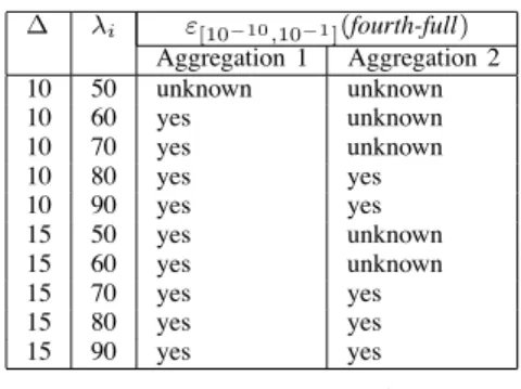
We verify the formula εI(fourth-full) in two different
inter-vals I, by computing Ru(fourth-full) and Rl(fourth-full). In
table I, we suppose that I = [10−10, 10−1], and we give the results of the verification for the two aggregation schemes. We have verified that for the two aggregation schemes, we are in the case that gu(E
yes) and gl(Eyes) are increasing sets, and
for the lower bound 2 is verified. As we have explained before, Aggregation1 is defined so as to provide more precise bounds values then Aggregation2. In tables III and IV, we can see that Markov chains sizes are larger with Aggregation1 then Aggregation2, and when ∆ increases, the sizes increases also. From table I, we can see that ε[10−10,10−1](fourth-full) is
in some cases unknown with Aggregation2, but true with Aggregation1, because the bounds are more precise. Another remark is that for an aggregation scheme, when ∆ increases, the precision improvement makes the state formula transits from an unknown response (Aggregation1, ∆ = 10, λi= 50)
to a positive response (Aggregation1, ∆ = 15, λi= 50).
For table II, given the same assumptions, we reduce the interval I which is now equal to I = [10−6, 10−2]. Clearly,
we can see globally that the verification is more often unknown then in the precedent case. Clearly, we couldn’t conclude
∆ λi ε[10−6,10−2](fourth-full) Aggregation 1 Aggregation 2 10 50 unknown unknown 10 60 unknown unknown 10 70 yes unknown 10 80 yes unknown 10 90 yes unknown 15 50 unknown unknown 15 60 yes unknown 15 70 yes unknown 15 80 yes unknown 15 90 yes unknown TABLE II
ε[10−6,10−2](fourth-full) :WITHAGGREGATIONS1, 2ANDBi= 20
Exact Aggregation1 Aggregation2 ∆=10 ∆=15 ∆ = 10 ∆=15 194481 158071 191751 61051 140091
TABLE III
STATE SPACE SIZE OF AGGREGATEDMARKOV PROCESSES FORB=20
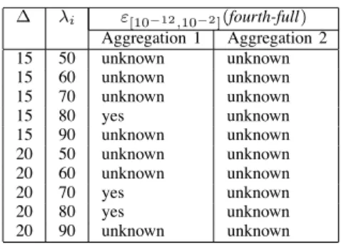
with Aggregation2, but the response can be obtained from Aggregation1, and with the increasing of ∆. The same remarks can be deduced from V and VI when we increase buffer sizes.
VI. CONCLUSION
In this paper, we have proposed a checker algorithm based on stochastic comparisons of multidimensional Markov chains. This algorithm has been applied to check state formulas with rewards defined on steady-state distribution, with CSRL logic. Quantitative analysis of large systems can be intractable if there is no specific solution as product forms. To overcome the state space explosion problem, we have proposed to use stochastic comparisons by mapping functions in order to define aggregated bounding Markov processes. We have defined an
Exact Aggregation1 Aggregation2
∆=15 ∆=20 ∆=15 ∆=20
2825761 1587311 2296141 438311 884101 TABLE IV
STATE SPACE SIZE OF AGGREGATEDMARKOV PROCESSES FORB=40
∆ λi ε[10−13,10−1](fourth-full) Aggregation 1 Aggregation 2 15 50 unknown unknown 15 60 yes unknown 15 70 yes unknown 15 80 yes yes 15 90 yes yes 20 50 unknown unknown 20 60 unknown unknown 20 70 yes yes 20 80 yes yes 20 90 yes yes TABLE V
ε[10−13,10−1](fourth-full)FORAGGREGATIONS1,2,ANDBi= 40
∆ λi ε[10−12,10−2](fourth-full) Aggregation 1 Aggregation 2 15 50 unknown unknown 15 60 unknown unknown 15 70 unknown unknown 15 80 yes unknown 15 90 unknown unknown 20 50 unknown unknown 20 60 unknown unknown 20 70 yes unknown 20 80 yes unknown 20 90 unknown unknown TABLE VI
ε[10−12,10−2](fourth-full)WITHAGGREGATIONS1, 2ANDBi= 40
algorithm which verify the state formulas using the upper and lower bounds generated by aggregated Markov processes. We have proposed a parametric aggregation in order to have a tradeoff between the size of the aggregated Markov chains and the accuracy of the bounds. This aggregation allows the checker algorithm to refine its verification by becoming closer to the exact model.
VII. REFERENCES
[1] S. Andova, H. Hermanns, J.P. Katoen, ”Discrete-time rewards model-checked”, Formats2003, LNCS 2791, 2003.
[2] C. Baier, B. Haverkort, H. Hermanns and J.P. Ka-toen, ”Model-Checking Algorithms for Continuous Markov Chains”, IEEE Transactions on Software Engineering, Vol. 29, NO. 6, June 2003.
[3] M. Ben Mamoun, N. Pekergin and S. Youn`es, ”Model Checking of Continuous Time Markov Chains by Closed-Form Bounding Distributions”, Qest’06.
[4] H.Castel, L.Mokdad, N.Pekergin, ”Aggregated bounding Markov processes applied to the analysis of tandem queues”, Second International Conference on Performance Evaluation Methodologies and Tools, ACM Sigmetrics, ValueTools 2007, October 23-25, 2007, Nantes, France.
[5] H.Castel, L.Mokdad, N.Pekergin, ”Stochastic bounds applied to the end to end QoS in communication systems”, 15th Annual Meeting of the IEEE International Symposium on Modeling, Analysis, and Simulation of Computer and Telecommunication Systems (MASCOTS 2007), October 24-26 2007, Bogazici University Istanbul, published by the IEEE Computer Society
[6] Clarke EM, Emerson A, Sistla A,P ,”Automatic verifi-cation of finite-state concurrent systems using temporal logic spacifications”, ACM Trans. on Programming Languages and Systems 8 (2) : 244-263, 1986
[7] M.Doisy, ”Comparaison de processus Markoviens”, PHD thesis, Univ. de Pau et des pays de l’Adour 92.
[8]J. M. Fourneau, N. Pekergin, ”An algorithmic approach to stochastic bounds”, in Performance Evaluation of Complex Systems: Techniques and Tools, LNCS 2459, 2002.
[9] J.M Fourneau, M. Lecoz, F. Quessette, ”Algorithms for irreducible and lumpable strong stochastic bound”, Linear Algebra and its Applications 386 (2004) 167-185, 2004.
[10] B.Haverkort,L.Cloth, H.Hermanns,J-P Katoen, C. Baiers, ”Model checking performability properties” Proc. of IEEE DSN’02, 2002.
[11] T.Lindvall, ”Lectures on the coupling method”, Wiley series in Probability and Mathematical statistics, 1992.
[12] T. Lindvall, ”Stochastic monotonicities in Jackson queueing networks”, Prob. in the Engineering and Informa-tional Sciences 11, 1997, 1-9.
[13] W. Massey, ”Stochastic orderings for Markov processes on partially ordered spaces” Mathematics of Operations Re-search, Vol.12, N2, May 1987.
[14] H.G. Perros, ”Queueing networks with blocking, exact and approximate solutions”, Oxford university press, 1994.
[15] N. Pekergin, ”Stochastic performance bounds by state space reduction”, Performance evaluation, 36-37, (1-17), 1999. [16] N.Pekergin, S.Younes, ”Stochastic model checking with stochastic comparison”, EPEW05, LNCS 3670, (109-124), 2005.
[17] D. Stoyan, ”Comparison methods for queues and other stochastics models”, J. Wiley and son, 1976.
[18] J.Sproston, S.Donatelli, ”Backward bisimulation in Markov chain model checking” , IEEE Transactions on Soft-ware Engineering, Vol. 32, NO.8, August 2006.
[19] W.J. Stewart, ”An Introduction to the Numerical Solu-tion of Markov Chains”, Princeton, 1993.
APPENDIX
A. Stochastic orderings theory
We present some theorems and definitions about stochastic orderings used for the generation of the aggregated bounding Markov chains.
Two formalisms can be used for the definition of a stochastic ordering : increasing functions [6,16] or increasing sets [12]. The *st ordering is the most known stochastic ordering,
it is equivalent to the sample path ordering (see Strassen’s theorem [16]. Stochastic orderings are defined only on discrete and countable state space E, where a binary relation * is defined at least as a preorder [16]:
We consider two random variables X and Y defined on E, and their probability measures given respectively by the probability vectors p and q where p[i] = P rob(X = i), ∀i ∈ E (resp. q[i] = P rob(Y = i), ∀i ∈ E). The *st ordering can
be defined using increasing functions as follows [16]: Definition 1: X *st Y ⇔ E[(f(X))] * E[(f(Y ))] ∀f :
E→ R, *-increasing whenever the expectations exist. Different methods are associated to the *st ordering: the
coupling [16], [10], and the increasing set theory [12]. We focus in this paper only on the *st ordering. The
key idea is to define a stochastic ordering from a family of increasing sets [12]. Let Γ⊆ E, we denote by
Γ ↑= {y ∈ E | y 2 x, x ∈ Γ}
Definition 2: Γ is called an increasing set if and only if Γ = Γ ↑
Let φst(E) the family of increasing sets which induces the
*st ordering:
φst(E) = {all increasing sets on E}
The *st ordering theorem using the increasing set theory
[12] states as follows: Theorem 1: X *stY ⇔ p *stq⇔ p(Γ) ≤ q(Γ), ∀Γ(φst(E) where p(Γ) =" x∈Γ p(x)
We present now the comparison of stochastic processes. Let {X(t), t ≥ 0} and {Y (t), t ≥ 0} stochastic processes defined on E.
Definition 3: We say that{X(t), t ≥ 0} *st{Y (t), t ≥ 0}
if X(t) *stY (t),∀t ≥ 0
As the stochastic comparison of processes is defined as the stochastic comparison at any time of the processes, then it is also equivalent to :
E(f (X(t))≤ E(f(Y (t)), ∀t ≥ 0
∀f : E → R, *-increasing whenever the expectations exist. Different methods can be used to define a stochastic order-ing : increasorder-ing sets and couplorder-ing [12,16,10].
Next, we suppose that the Markov processes are not defined on the same state spaces. In this case, we can compare them on a common state space using mapping functions. The relevance of this technique is to reduce the state space of the Markov chains in order to define bounding aggregated Markov chains. Let :
• X(t) a Markov process defined on E, we suppose that
the stationary distribution Π1 exists.
• Y (t) a Markov process defined on S⊂ E), we suppose
that the stationary distribution Π2 exists. • g be a many to one mapping from E to S.
The stochastic comparison of these processes by mapping functions is defined as follows [6]:
Definition 4: We say that
{g(X(t)), t ≥ 0} *st{Y (t), t ≥ 0}
if g(X(t)) *stY (t),∀t ≥ 0
If the state space S ⊂ E, then this theorem allows to compare the process X(t) with the process Y (t) defined on a smaller state space.
Proposition 1: If
{g(X(t)), t ≥ 0} *st{Y (t), t ≥ 0}
" g(x)∈Γ Π1(x)ρ(x) ≤ " x∈Γ Π2[x]ρ(x), ∀Γ ∈ Φst(S)
where ρ : E→ R>0, an increasing function.
B. Propositions, theorems proofs Proposition 2: " x∈Eyes Π[x] ≤ " x|g(x)∈g(Eyes) Π[x] Proof " x|g(x)∈g(Eyes) Π[x] = "
x∈Eyes|g(x)∈g(Eyes)
Π[x]
+ "
x'∈Eyes|g(x)∈g(Eyes)
Π[x] as ∀x ∈ Eyes, g(x)∈ g(Eyes), then clearly we have :
"
x∈Eyes|g(x)∈g(Eyes)
Π[x] = "
x∈Eyes
Π[x] and so we deduce that :
"
x∈Eyes
Π[x] ≤ "
x|g(x)∈g(Eyes)
Π[x]
Here we give a simple example about this proposition. Example 1: Let E ={(0, 0), (1, 0), (0, 1), (1, 1)}, with the preorder component by component. The mapping g : E → S where s ⊂ E is such that : g(0, 0) = (0, 0), g(0, 1) = g(1, 0) = g(1, 1) = (1, 1). So S ={(0, 0), (1, 1)}.
For Eyes = {(0, 1)}, then g(Eyes) = {(1, 1)}, which
is an increasing set, and !x∈EyesΠ[x] = Π[(0, 1)] ≤
!