HAL Id: hal-01333408
https://hal.archives-ouvertes.fr/hal-01333408
Submitted on 17 Jun 2016
HAL is a multi-disciplinary open access
archive for the deposit and dissemination of
sci-entific research documents, whether they are
pub-lished or not. The documents may come from
teaching and research institutions in France or
abroad, or from public or private research centers.
L’archive ouverte pluridisciplinaire HAL, est
destinée au dépôt et à la diffusion de documents
scientifiques de niveau recherche, publiés ou non,
émanant des établissements d’enseignement et de
recherche français ou étrangers, des laboratoires
publics ou privés.
Dealing with Large MDPs, case study of waterway
networks supervision
Guillaume Desquesnes, Guillaume Lozenguez, Arnaud Doniec, Eric Duviella
To cite this version:
Guillaume Desquesnes, Guillaume Lozenguez, Arnaud Doniec, Eric Duviella. Dealing with Large
MDPs, case study of waterway networks supervision.
14th International Conference on
Practi-cal Applications of Agents and Multi-Agent Systems, PAAMS, Jun 2016, Séville, Spain. pp.48-59,
�10.1007/978-3-319-39324-7_5�. �hal-01333408�
Draft: Dealing with Large MDPs, case study of
waterway networks supervision
Guillaume Desquesnes, Guillaume Lozenguez, Arnaud Doniec, and Eric Duviella
Mines Douai, IA, F-59508 Douai, France, Univ. Lille, F-59500 Lille, France [email protected]
Abstract. Inland waterway networks are likely to go through heavy changes due to a will in increasing the boat traffic and to the effects of cli-mate change. Those changes would lead to a greater need of an automatic and intelligent planning for an adaptive and resilient water management. A representative model is proposed and tested using MDPs with promis-ing results on the water management optimization. The proposed model permits to coordinate multiple entities over multiple time steps in or-der to avoid a flood in the waterway network. However, the proposed model suffers a lack of scalability and is unable to represent a real case application. The advantages and limitations of several approaches of the literature are discussed according to our case study.
Keywords: Markov Decision Process, Inland waterway network, Large model
1
Introduction
Climate change is a main concern in our modern society. In the last years, the effects of global change on the inland waterway network has been studied. The general agreement is that the intensity and the occurrence of flood and drought periods will increase [17].
In parallel, the use of inland navigation to decongest road and railway traffic is in vogue. An increase of ships traffic is thus expected in the coming years. All these evolutions tend to complicate the water management in inland waterway networks and make human planning less and less relevant.
An inland waterway network is an artificial water system interacting with the natural environment. Most of these interactions are only partially known: illegal discharges, exchanges with groundwater tables, local weather influence, . . . The control of a such a network is thus subjected to uncertainties and a stochastic modeling seems therefore more adapted.
Markov Decision Processes (MDPs) are widely used for planning on stochas-tic models and provide plan for all configurations of the model. To the best of our knowledge, MDPs have not yet been used to model the inland waterway net-work in order to make them resilient and more stable. However previous net-work
II
has been made on this topic, using flow network with the strong hypothesis of a deterministic model [16].
MDP framework permits to model the evolution of an uncertain system but induces intractable model in most of the applications. Those large MDPs make the policies of an optimal control hard to compute and require specific algo-rithms [3,15]. A stochastic modeling of the network is proposed, allowing to plan a coordination of all entities in the network. The main complexity comes from the distribution of water transfer possibilities over a territory. An optimal con-trol represents all possible join water transfers considering all complete network situations. This paper aims to draw back the limitations of such an optimal cen-tralized model applied to waterway network and to discuss about approaches that take advantage of distributed control.
In this paper, the problem of inland waterway network management in a context of climate change is presented in section 2. A naive modeling of the network using MDP is proposed in section 3 and some results and the limitations are shown in section 4. Finally a description and comparison of MDP approaches for large scale and distributed model is proposed in section 5 with regard to inland waterway network supervision.
2
Waterway Network Supervision
An inland waterway network, see figure 1a is a large scale system, mostly used for navigation. It provides both economic and environment benefits [13,14] while providing quiet, efficient and safe transports of goods [5]. It is mostly composed of
(a) Small part north of France inland waterway net-work
Navigation Rectangle
NNL HNL
LNL
(b) Navigation rectangle
canalized rivers and artificial channels, and is divided by locks. Any part between two locks is called a navigational reach. For the sake of simplicity, navigational reach will be called reach on the rest of this paper.
The water level of a reach must respect the conditions of the navigation rectangle, see figure 1b, and be as close as possible from the Normal Navigation Level (NNL). The lower and upper boundaries of the rectangle are respectively
III the Lower and Higher Navigation Level (LNL & HNL). The main concern of the operator consists in maintaining acceptable water level in all the reaches of the inland waterway network.
In normal situation, having a boat crossing a lock is the main disturbance of the water level, since using a lock drains water from the upstream reach and release water to the downstream reach. Furthermore the water level is affected by ground exchanges, natural rivers, weather and other unknown factors, like illegal discharges. Locks are not dedicated to control the water level, so gates are used to send water downstream and pumps can be used to send some upstream.
At the moment, the navigation is only allowed during daytime, with few ex-ceptions, notably on Sunday. Reaches management is based on human expertise gathered over the time. But in a context of climate change, that will increase the effect of floods and droughts, and with a will to increase the traffic, notably by allowing 24 hours a day traffic, those methods start to show their limits.
The objective is to determine a global planning, to maintain the navigation conditions in the entire network, by taking into account uncertainties of the problem, such as weather and traffic in a context of climate change and increasing navigation traffic. Planning over multiple time steps allows a better anticipation of possible events and a better reaction over unexpected events, using real-time information of the network using level sensors spread through the reaches.
3
Using Markov Decision Process
Markov Decision Process (MDP) is a generic framework modeling control possi-bility of stochastic dynamic system as probabilistic automaton. The framework is well adapted to Waterway Network Supervision while the state of the network is fully observable (in term of water volumes) and the control is uncertain due to uncontrolled water transit.
3.1 MDP model
A MDP is defined as a tuple hS, A, T, Ri with S and A respectively, the state and the action sets that define the system and its control possibilities. T is the transition function defined as T : S × A × S → [0, 1]. T (s, a, s0) is the probability
to reach the state s0 from s by doing action a ∈ A. The reward function R is defined as R : S × A × S → R, R(s, a, s0) gives the reward obtained by attaining s0 after executing a from s.
A policy function π : S → A assigns an action to each system state. Optimally solving a MDP consists in searching an optimal policy π∗ that maximizes the expected reward. π∗maximizes the value function of Bellman equation [1] defined on each state: Vπ(s) = X s0∈S T (s, a, s0) × ( R(s, a, s0) + γVπ(s0) ) with a = π(s) (1) π∗(s) = arg max a∈A ( X s0∈S T (s, a, s0) × ( R(s, a, s0) + γVπ∗(s0) ) ) (2)
IV
The parameter γ ∈ [0, 1] balances the importance between future and imme-diate rewards. With γ set close to 0 the immeimme-diate action with the maximal re-ward will be taken while a γ close to 1 will permit the control to accept penalties if future gains could be important. Multiple algorithms exist to solve optimally a MDP, a notable version is Value Iteration [19]. It constructs iteratively the value function V , using equation 3, until convergence or until a specified number of iterations has been done. The last Vi obtained is then used to generate the
optimal policy with equation 2. The first value function, V0 is initialized at 0.
Vi+1(s) = max
a∈A(
X
s0∈S
T (s, a, s0) × ( R(s, a, s0) + γVi(s0) ) ) (3)
3.2 Naive Waterway Network Control
The objective is to plan the best course of actions for the whole network over t time steps, knowing that some conditions may differ on each time step and can affect the inland navigation. For instance the weather might become rainy which will increase the water volume of affected reaches or more boats than expected could traverse the reach resulting in an higher lock usage.
N represents the number of reaches in the network. Since large time steps are used, we make the assumption that the water level is the same or nearly same at all point in a reach.
A state of the model is defined as an assignation of volume for all the reaches in the network at a given time. Similarly an action is defined as an assignation of volume for each controlled point of transfer (locks, pumps and gates). The MDP formalism requires discrete set of states and actions, but since the volumes are continuous, we discretized them using intervals.
Each reach is divided in intervals, all of the same size, except the first and the last intervals which gather values that are outside of the navigation rectangle. Those two are considered to be of infinite size and represents everything that must be avoided at all cost. The water transfer points use a similar partition as the reaches, except that there is no infinite size intervals, since it is supposed to be fully controlled. More formally, the set of states S of the model is defined as the combination of all possible reaches volumes intervals for all time steps.
For a reach i, the intervals result from a regular discretization of volumes from less water than minimal authorized 0 to more than the maximal authorized riout.
S = {1, . . . , t} ×
N
Y
i=1
[0, riout] (4)
In a similar way, we define the set of actions A as the discretized volumes planed for transfer between between two adjacent reaches. Action is time inde-pendent, so we simply have
A = Y
i,j∈[0,N ]2
V where Li,j represent the set of all possible volume transfer of the transfer point
linking reach i to reach j and reach 0 represents external rivers linked to the reaches. In fact, there is only a limited number of transfer points and most of the Li,j do not permit any controlled transfer (Li,j= ∅).
We denote ai,j ∈ Li,j the transfer volume planed from reach i to reach j
in the action a ∈ A. To simplify the notation, ai defines the part of the action
affecting the reach i as
ai = N
X
j=0
( ai,j aj,i) (6)
We define two operators ⊕ and on (R ∪ I)2 → R, that can respectively
add and substract intervals of numbers and/or numbers, the result being alway a real.
I being the set of all possible intervals of our network. Our operators are respectively a simple addition and subtraction using the value of the member if it is a real, or its average value if it is an interval.
Our transition function T (s, a, s0) represent the probability to reach the state s0 by doing action a from the state s and taking into account the possible tem-poral variation. It results from discussions with experts of the north of France waterway network. Trivially, for s at time step t and s0 at time step t0, s0 is only reachable if t0 = t + 1.
Since the transition of each reach is independent from other reach, it only depends on the previous state and its incoming and outgoing water. A first source of uncertainty comes from the uncontrolled water modeled as a list of the temporal variations, noted Var .
Temporal variations are local changes to one or more reaches or transfer points during one or more time steps with some probabilities, for example rain on a reach is a temporal variation. Since those temporal variations are not repre-sented in the action space nor in the state space, they only affect the transition function. The uncontrolled volume of water affecting the reach i is noted vi∈ Var
and P (vi|t) represents the probability that the random variable vioccurs in time
step t. P (vi|t) is built based on data of uncontrolled water displacement
com-bined with weather forectasts.
The second source of uncertainty results from the discretization in interval of volume, causing an approximation in the state representation.
Let define P (ris0|ris, ai+ vi) the probability that the volume of water in
reach i at time step ts+ 1 will be included in interval ris0 if the action ai is
performed and with vi uncontrolled transfer on i:
P (ris0|ris, ai+ vi) = p= if ris⊕ ai+ vi ∈ ris0 p+ if ris⊕ ai+ vi∈ ris0+ 1 p− if ris⊕ ai+ vi∈ ris0− 1 0 else (7)
where p= is the probability to get the expected volumes by taking into account
VI
corresponding to a superior (resp. inferior) water level, with respect to
p++ p−+ p== 1 and p+= p−
The transition function states the product of the two sources of uncertainty:
T (s, a, s0) = N Y i=1 X ∀vi∈Var P (vi|t) × P (ris0|ris, ai+ vi) ! (8)
Finally, we define a reward function, representing the current goal of the operators, to greatly penalize the distance to the normal navigation level for each reach with a small cost for all water movement. More formally we define :
R(s, a, s0) = −1 × N X i=1 (NNLi ris0)2+ ai ! (9)
where NNLi is the volume corresponding to reach i being at normal navigation
level. If ris0 is outside the navigation rectangle we replace it by a large value c
and half this value if ris0 is only partially outside the navigation rectangle.
4
Test on a network
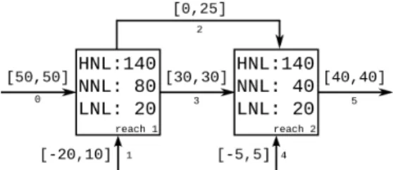
To test this approach, we made a realistic waterway network (see figure 2), with two reaches and six transfer points. Then the MDP is solved and the policy is tested on several scenarios.
Fig. 2: Waterway network
4.1 Network characteristics
On figure 2, the reaches represented by squares, with a specified volume range, in units of volume, and the arcs correspond to the transfer point with a minimum and maximum capacity. A negative value meaning this transfer point can be
VII used to import and export water. We simulate this network for 8 day and night periods, with locks closed during the night, giving us 16 time steps.
The two reaches volumes are divided in 9 intervals, 7 of size 20 and 2 of infinite size. The points of transfer 1, 2 and 4 are divided in intervals of size 5 (respectively 6, 5 and 2 intervals). The points of transfer 0, 3 and 5 transfer a constant amount of water. Since we were planning on 16 time steps, we had 9 × 9 × (16 + 1) = 1377 states. An extra time step is added to mark the end of the last planning step, all states within this time step are absorbing, which means T (s, a, s) = 1 and have R(s, a, s) = 0 to have no influence on the planning. In a similar way, the number of actions is 6 × 5 × 2 = 60.
We used c = 10000 as an arbitrary large value for being outside of the navigation rectangle. To valide the performances of our model, the probabilities of the intervals has been set arbitrarily to p== 0.9 and p+= p−= 0.05.
4.2 Some results
To analyze empirically the quality of the policy generated, we made a few simu-lations. We made 4 scenarios, the first one being an ideal scenario : both reaches start from their NNL and there is no perturbation. The second scenario consists of the first reach starting from its lowest bound and the second from its highest bound, still with no temporal perturbation. The third one is the opposite of the second one first reach from its highest, second from its lowest. And finally the last scenario is similar to the first one, except that during one time step an heavy rain may happen, with high probability, and would overflow the first reach if nothing is done to prevent it.
Since the policy actions are intervals, we decided to test our scenarios using random values from the chosen intervals to apply to the transfer points, rather than the best at the moment or the average value of the interval to test the quality of the chosen interval. Running each simulation 5 times allowed us to reduce the randomness impact while preserving clarity. It is important to note that the simulations use a continuous modeling of the systems, in both reaches volumes and transfered volumes.
We created our network so that the optimal policy of the first scenario would allow to maintain both NNL at all time steps. We can see in figure 3a, that we are only close from it. This is caused by our discretization. Since we represent an interval by its average value, it is possible for a reach to reduce or increase its level while not changing its state causing the reach to continue to decrease or increase its level.
The reaction of the network to some event that put the two reaches on the extremity of their navigation levels, is visible in figure 3b and 3c. We notice that the recovery is way faster in the second case because the upstream reach has to empty itself and the downstream needs to be filled unlike the second case where the opposite scenario is happening and each reach has to maintain a minimum impact on the other one to avoid making the other outside of its navigation level. In the last scenario, heavy rain is supposed to happen between step 7 and 8 causing the first reach to overflow if it is close to its NNL. And to prevent that we
VIII
(a) From NNL no perturbation (b) From LNL & HNL no perturbation
(c) From HNL & LNL no perturbation (d) From NNL with perturbation Fig. 3: Different scenarios
see that, few time steps before the event, the first reach will empty itself in the second reach, making it go further from its NNL but by doing that preserving the integrity of the system, if the perturbation happens.
4.3 Limitations in scaling up
A naive implementation of the transition function consists in creating a |S|2×|A| matrix, which would contain 13772× 60 = 1.137 677 40 × 108values, assuming 8
bytes to store each value would mean approximatively 0.91 GB of memory space only for the transition function.
Since, doing an action means that the time step will change, except on the dummy time step, only a small subset of the states, containing at most t+1|S| states can be reached. A sparse matrix would allow us to reduce drastically the size of the matrix, since only non zero values and their indices has to be stored, so as long as more than half of the matrix is empty, using the sparse matrix is beneficial. By calculating the optimal policy of our example, we have been able to observe a few results. Firstly it converges very fast and works as intended but the construction of the transition function takes most of the time. Since time isn’t cyclic, it is possible to find the optimal action for all states corresponding to a certain time step, if it is the last one or if the next one already has optimal action for the states. This allow us to add a max bound to the number of iterations required to find the optimal policy to the number of time steps, here 17.
IX
5
Approaches to Workaround Naive Model Limitation
By increasing the size of our example or its precision, we quickly encounter memory limitations. Furthermore, the state domain, by construction, grows ex-ponentially in the number of reaches and, real application such as the inland waterway network in north of France contains around 50 reaches. Our naive approach wouldn’t be able to calculate an optimal policy for this application.
To workaround spatial limitations, some extensions of the MDP have been defined in the literature such as a factored representation of the model. An other technique consist in decomposition where the MDP is split into local sub-MDPs. Investigation focus on approaches permitting to plan a policy covering the entire state space. For now, we are not interested in approximation as based on Monte-Carlo tree-search [11] where the computed policy fit only probable states. This approach requires to know the initial states and a continuous mechanism if the system derives toward uncover states.
5.1 Factored MDP
The factored MDP approach aims to represent in a compact way the transition and reward functions, as introduced by Boutilier, Dearden, Goldszmidt et al. [4]. For that purpose states are represented by an assignation of variables. Every variables may have no influence on the value of a specific variable at the next time step. The idea behind factored MDPs is to explode the state space to group similar part of states in the transition and reward functions.
Hoey, St-Aubin, Hu and Boutilier [10] use algebraic decision diagram (ADD) to represent in a more compact way transition, reward and value functions by capturing regularity in the respective function.
Guestrin, Koller and Parr used factored MDP to solve multi agent planning in [8]. They approximate the value function as a linear combination of localized value functions. Their method exploits both state and action space structure. This allows to solve problems with over 1028 states and a 109 actions.
Fur-thermore agents need a coordination graph, to decide their action on runtime. However this approach assumes that agents interact only with a few of other agents.
This limitation is bypassed by a rule-based approach introduced by Guestrin, Venkataraman and Koller in [9], this approach worst case being faster than the previous approach worst case, nevertheless in some case the previous approach is faster. Furthermore the rule-based approach doesn’t require the rules to be mutually exclusive unlike tree or ADD representation.
In our case, the state space (resp. action space) results in the cartesian prod-uct of the state space (resp. action space) of each reach. But the state of a reach usually doesn’t depends directly on the state of nearby reaches, only their ac-tion matters, when a reach receive water, the volume of the source isn’t used to determine its new level. Since we assume moving water is always possible, reach never full nor empty, because such action are forbidden in the model, the state of reaches are independant and we could exploit it to factorize our MDP.
X
5.2 Decomposed MDP
The decomposition of an MDP permits to decrease the complexity of the policy computation by building a hierarchy between local problems and a global so-lution [3,7]. It is particularly efficient in spatial problems as it is based on the topological aspect of transitions.
Decomposed MDP splits the state spaces into sub-MDPs in a way the union of sub-MDPs cover the total MDP. Dean et al. [7] proposed two approaches to solve Decomposed MDP. The first iterative approach consists in solving each sub-MDP iteratively until a stable point is reached. A stable point match that all the sub-policies are coherent among each other. This solution do not guaranty to speed-up the policy computation but guaranty the optimality of the total policy (the union of sub-policies).
The second hierarchical approach consists in defining a set of parameters for each sub-MDPs in order to compute a finite collection of sub-policies. Then, a high level global MDPs is defined on “macro-states” to select the appropriates sub-policies to apply in order to have a coherent global behavior. This solution permits to control the policy computation but does not guaranty the optimality of the solution. The quality of the total policy take benefit from rich parameter definition but, with a cost on the computation resources.
In most real problems, Decomposed MDP could reduce policy computation (with or without optimal guaranty) but require to compute a partition in the state space [18,20]. If there are no evident decomposition, partitioning is a very hard [2], and could penalize a decomposition approach.
Waterway MDP is not easily decomposable while each state represents a snapshot of the entire networks. However, an option exists in considering sev-erals levels of deterioration of navigation conditions. Each sub-MDP matching deteriorate condition will produce a policy of supervision oriented to the normal navigation conditions. For example with a Waterway MDP decomposed in tree sub-MDP: normal, flood and drought, we can expect that the supervision policy will keep the system in normal states (close to NNL) with spare dependencies be-tween the tree sub-MDPs. This way, solving first the normal sub-MDP and them the two deteriorate sub-MDP will speed-up the policy computation. However, decomposition will not impact transition function construction and storage.
5.3 Distributed MDP
Distributed MDPs appear as ad-hoc solution to solve cooperative problems on agent based modeling. Such an approach is developed to solve Decentralized MDP [6,15] (a framework where the policy have to be distributed over agents and performed in a decentralized way). Each agent is responsible in computing its own policy considering its part of a mission. Protocols based mechanisms allow the agents to adapt their policies to reach a common interest. Distributed MDP is used for example in robotic mission to deal with traveling salesmen coordination [12].
XI This approach combines factorization and decomposition ideas. The total MDP is split in several sub-MDP by partitioning the set of variables defining the states and actions. Each sub-MDP is responsible for a subset of problem variables and ignores the others. In agent based modeling, each sub-MDP will match agent capability in the group (individual perceptions and actions).
An iterative approach is used to solve Distributed MDP while each iteration will modify each sub-MDP structure (transition and/or reward values). The computation is stopped when policies are stable for all the sub-MDPs (agents). The state space explored to compute the policy could be significantly reduced. That permit to speed-up computation, however, they are no guaranty on the optimality of the solution.
Waterway network would be easily distributable as the transit points are already distributed over a territory. An agent in the agent based model will be responsible for the control of one or few connected transit points and the coordi-nation mechanism will be based on the reaches which are common to two or more agents. Distributed MDP seems very promising, for our problematic, because it can significantly decrease computation complexity and it allows flexible network definition. However, the result by using such an approach remain uncertain con-sidering that distributed MDP solving is a young approach with mostly ad-hoc contribution to specific application and no generic framework established yet.
6
Conclusion
In this paper, we present a MDP based approach to optimize the water manage-ment in inland waterway network with a global view and planning on a given horizon. This approach aims to reduce the impact of drought and flood that may be increased by climate change in the next years.
Using MDPs, it is possible to model the dynamic and the uncertainty in such a system to optimize navigation conditions. However, this model is quickly limited by the size of the state space and thus we presented possible trails to circumvent this limitation. We investigated Factored MDP, Decomposed MDP and Distributed MDP. Factored and Distributed MDP take advantage to variable correlations in state and action definitions. Variable correlation is relevant in distributed problems as water management in inland navigation.
In future works, we plan to explore Distributed MDP based on an agent modeling of the waterway network even though this solution does not guarantee the optimality. We expect a better control of the required computation resources which is required to handle any size of networks. Determining the probability to reach the expected interval will also be explored, alongside the discretization.
References
1. Bellman, R.: A Markovian Decision Process. Journal of Mathematics and Mechan-ics 6, 679–684 (1957)
XII
3. Boutilier, C., Dean, T., Hanks, S.: Decision-theoretic planning: Structural assump-tions and computational leverage. Journal of Artificial Intelligence Research 11, 1–94 (1999)
4. Boutilier, C., Dearden, R., Goldszmidt, M., et al.: Exploiting structure in policy construction. In: IJCAI. vol. 14, pp. 1104–1113 (1995)
5. Brand, C., Tran, M., Anable, J.: The uk transport carbon model: An integrated life cycle approach to explore low carbon futures. Energy Policy 41, 107–124 (2012) 6. Chades, I., Scherrer, B., cois Charpillet, F.: A Heuristic Approach for Solving Decentralized-POMDP: Assessment on the Pursuit Problem. In: SAC ’02: Pro-ceedings of the 2002 ACM symposium on Applied computing. p. 5762. ACM, New York, NY, USA (2002)
7. Dean, T., Lin, S.h., Lin, S.h.: Decomposition Techniques for Planning in Stochastic Domains. In: 14th International Joint Conference on Artificial Intelligence (1995) 8. Guestrin, C., Koller, D., Parr, R.: Multiagent planning with factored mdps. In:
NIPS. vol. 1, pp. 1523–1530 (2001)
9. Guestrin, C., Venkataraman, S., Koller, D.: Context-specific multiagent coordina-tion and planning with factored mdps. In: AAAI/IAAI. pp. 253–259 (2002) 10. Hoey, J., St-Aubin, R., Hu, A., Boutilier, C.: Spudd: Stochastic planning using
decision diagrams. In: Proceedings of the Fifteenth conference on Uncertainty in artificial intelligence. pp. 279–288. Morgan Kaufmann Publishers Inc. (1999) 11. Kocsis, L., Szepesvri, C.: Bandit Based Monte-Carlo Planning. In: Frnkranz, J.,
Scheffer, T., Spiliopoulou, M. (eds.) Machine Learning: ECML 2006, p. 282293. Lecture Notes in Computer Science, Springer Berlin Heidelberg
12. Lozenguez, G., Adouane, L., Beynier, A., Mouaddib, A.I., Martinet, P.: Punctual versus continuous auction coordination for multi-robot and multi-task topological navigation. Autonomous Robots p. 115 (2015)
13. Mallidis, I., Dekker, R., Vlachos, D.: The impact of greening on supply chain design and cost: a case for a developing region. Journal of Transport Geography 22, 118– 128 (2012)
14. Mihic, S., Golusin, M., Mihajlovic, M.: Policy and promotion of sustainable inland waterway transport in europe–danube river. Renewable and Sustainable Energy Reviews 15(4), 1801–1809 (2011)
15. Nair, R., Varakantham, P., Tambe, M., Yokoo, M.: Networked Distributed POMDPs: A Synthesis of Distributed Constraint Optimization and POMDPs. In: National Conference on Artificial Intelligence. p. 7 (2005)
16. Nouasse, H., Rajaoarisoa, L., Doniec, A., Duviella, E., Chuquet, K., Chiron, P., Archimede, B.: Study of drought impact on inland navigation systems based on a flow network model. In: Information, Communication and Automation Technolo-gies (ICAT), 2015 XXV International Conference on. pp. 1–6. IEEE (2015) 17. Pachauri, R.K., Allen, M., Barros, V., Broome, J., Cramer, W., Christ, R., Church,
J., Clarke, L., Dahe, Q., Dasgupta, P., et al.: Climate change 2014: Synthesis report. contribution of working groups i, ii and iii to the fifth assessment report of the intergovernmental panel on climate change (2014)
18. Parr, R.: Flexible Decomposition Algorithms for Weakly Coupled Markov Decision Problems. In: 14th Conference on Uncertainty in Artificial Intelligence. p. 422430 (1998)
19. Puterman, M.L.: Markov Decision Processes: Discrete Stochastic Dynamic Pro-gramming. John Wiley & Sons, Inc. (1994)
20. Sabbadin, R.: Graph partitioning techniques for Markov Decision Processes de-composition. In: 15th Eureopean Conference on Artificial Intelligence. p. 670674 (2002)