HAL Id: hal-01962218
https://hal.archives-ouvertes.fr/hal-01962218
Submitted on 20 Dec 2018
HAL is a multi-disciplinary open access
archive for the deposit and dissemination of
sci-entific research documents, whether they are
pub-lished or not. The documents may come from
teaching and research institutions in France or
abroad, or from public or private research centers.
L’archive ouverte pluridisciplinaire HAL, est
destinée au dépôt et à la diffusion de documents
scientifiques de niveau recherche, publiés ou non,
émanant des établissements d’enseignement et de
recherche français ou étrangers, des laboratoires
publics ou privés.
Adaptive Time, Monetary Cost Aware Query
Optimization on Cloud Database Systems
Chenxiao Wang, Zach Arani, Le Gruenwald, Laurent d’Orazio
To cite this version:
Chenxiao Wang, Zach Arani, Le Gruenwald, Laurent d’Orazio. Adaptive Time, Monetary Cost Aware
Query Optimization on Cloud Database Systems. International workshop on Scalable Cloud Data
Management (SCDM@BigData), Dec 2018, Seattle, United States. �hal-01962218�
Adaptive Time, Monetary Cost Aware Query Optimization on Cloud Database
Systems
Abstract--Most of the existing database query optimization
techniques are designed to target traditional database systems with one-dimensional optimization objectives. These techniques usually aim to reduce either the query response time or the I/O cost of a query. Evidently, these optimization algorithms are not suitable for cloud database systems because they are provided to users as on-demand services which charge for their usage. In this case, users will take both query response time and monetary cost paid to the cloud service providers into consideration for selecting a database system product. Thus, query optimization for cloud database systems needs to target reducing monetary cost in addition to query response time. This means that query optimization has multiple objectives which are more challenging than one-dimensional objectives found in traditional paradigms. Similar problems exist when incorporating query re-optimization into the query execution process to obtain more accurate, multi-objective cost estimates. This paper presents a query optimization method that achieves two goals: 1) identifying a query execution plan that satisfies the multiple objectives provided by the user and 2) reducing the costs of running the query execution plan by performing adaptive query re-optimization during query execution. The experimental results show that the proposed method can save either the time cost or the monetary cost based on the type of queries.
Keywords—Query Optimization, Cloud Computing, Cloud database
I. INTRODUCTION
Query optimization on a cloud database differs from optimization on a traditional distributed database for several reasons. First, a cloud database is provided to the user via a leasing service with several options of payment [5]. The user would need to take the monetary cost paid to the cloud service provider for query processing into consideration on top of the query response time. While in traditional database query optimization, the monetary cost is usually negligible because the infrastructure configuration is fixed and the monetary cost is paid up-front. Thus, in the usage of a cloud database system, the user can provide both the query response time limit and monetary budget of a query, which are defined as User
Constraints. Query optimization becomes multi-objective to
satisfy multiple user constraints [5]. Secondly, a cloud database is elastic. Cloud service providers provide a finite pool of
virtualized on-demand resources [11]. Similarly, users can decide the number and types of containers on which they would like to run their queries, and they can change the combination of container types over time. If users select more containers or more powerful containers, the time cost of the query execution may decrease, but the monetary cost may increase. That is, the time cost often contradicts the monetary cost. Query optimization on cloud databases should balance both time and monetary cost so that the users can obtain the result of the query with all the user constraints are satisfied. So, cloud database systems are responsible for providing the users with a feasible query optimization solution to deliver the query results that satisfy the user constraints as well as minimize the multiple costs of query execution. Besides that, the time and monetary costs needed to execute a query are estimated based on the data statistics that the query optimizer has available when the query optimization is performed. These statistics are often not accurate, which may result in inaccurate estimates for the time and monetary costs needed to execute the query [2]. Thus, the query execution plan (QEP) generated before the query is executed may not be the best one. Adaptively optimizing the QEP during the query execution to employ more accurate statistics will yield better QEP selection, and thus will improve query performance. There are some existing techniques that address part of these issues, which is that the selected QEP is suboptimal ([1][2][4][5][3][12][13][18][20]). However, they did not optimize queries based on both time and monetary costs and did not take adaptive optimization into consideration.
Optimizing a query on a cloud database environment requires an important consideration. Since the query will be executed on multiple nodes, one must consider how to allocate computational resources optimally, as there are an infinite number of workload/node combinations. However, not all the allocation solutions are feasible. Users will have query constraints, and resource allocation will strongly influence performance. Thus, optimal resource allocation becomes a problem, known simply as the scheduling problem [16][17]. The scheduling algorithm is also applied to resource allocation on cloud systems [9]. Besides that, good data statistics are critical to deriving a good schedule. They will affect the overall performance of query execution, as a sub-optimal query execution schedule will be produced by the optimizer if data statistics are erroneous. An effective schedule is based on accurate cost calculations of the tasks to be scheduled. It would
Chenxiao Wang
1Zach Arani
1Le Gruenwald
1Laurent d'Orazio
21 School of Computer Science
University of Oklahoma Norman, Oklahoma, USA
{chenxiao, myrrhman, ggruenwald}@ou.edu
2 CNRS,IRISA
Rennes 1 University Lannion, France
be beneficial if we could use the actual runtime query statistics instead of their estimates in the query optimization process. This is because estimates may not be as accurate as the actual running statistics. However, existing techniques either focus on optimizing queries based only on time, which is not sufficient for cloud database environments [2][3][6][19], or do not consider query re-optimization for more accurate statistics [7][12][13][21][22].
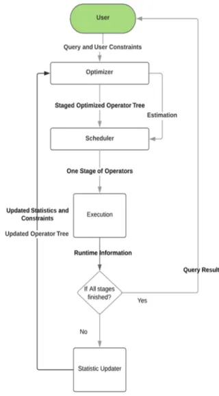
In this paper, we present an approach that adaptively optimizes queries based on query execution time and monetary costs. This approach will first generate multiple QEPs with different time and monetary costs. Each QEP is assigned a score using the Normalized Weighted Sum Algorithm (NWSA) based on its time and monetary cost estimation [20]. By using the NWSA model, a QEP that satisfies both the user constraints of time and monetary costs can be easily found. The estimated execution time and monetary cost of each QEP are normalized using user-defined maximum values for each objective. The score is the accumulation of these normalized value. The QEP with the lowest score is then selected and will be executed stage by stage. After a stage is executed, the statistics will be updated and used to re-optimize the remaining stages until all stages are executed and the query is finished. The procedure is captured in Fig. 1.
The rest of the paper is organized as follows. Section II discusses the related work. Section III formulates the query execution plan optimization problem. Section IV presents the proposed adaptive query optimization method. Section V presents the experimental results comparing our approach with the case when no adaptive query optimization is employed. Finally, Section V provides the conclusions and future research.
II. RELATED WORK
A. Adaptive query optimization
There are existing query optimization techniques that adopt re-optimization during execution ([2][6][19]). Bruno et al. [2] have proposed a query optimization method during query execution. The query execution is paused for multiple times at points defined by the re-optimization policy. At each of the points, a new estimation of the cost to execute the remaining query parts is made with the statistics collected from the finished parts of the query. The unexecuted parts of the query are adjusted with the new estimation. The adjusted query applies more accurate estimations, improving query performance. Costa et al. [6] proposed an adaptive optimization algorithm which dynamically adjusts the number of nodes. First, the optimizer estimates the finishing time of the current query periodically. Whenever the optimizer detects that the finishing time violates the service level agreement (SLA)—which is an agreement between the user and cloud provider—the query will be re-optimized and one new computational node will be added to participate in query execution. Otherwise, the query continues to
be executed. Liu et al.[19] have proposed a method that enables
queries to be optimized by runtime conditions. The re-optimization is incremental, meaning it does not require the whole query to be generated from the beginning. The executed part of the QEP will be pruned from the search space and a new QEP will be generated based on the unfinished part of the old one. This new QEP will be added to the search space and the algorithm will find the optimal QEP from the new search space.
This will significantly reduce the overhead of doing re-optimization. These existing approaches ([2][6][19]) optimize the QEP adaptively, but the objective is only based on the query response time, while our work is aimed at both the query response time and monetary cost.
B. Multi-objective query optimization
Some existing techniques optimize the query execution plan not only based on query response time but also based on other costs of executing the query ([1][5][7]). Kllapi et al. [1] have proposed a method that can schedule any dataflow on a set of containers to form one (or more) schedule(s). This means the estimation of time and monetary cost of executing this schedule will satisfy multi-user constraints. This algorithm assumes that the dataflow is available in a Directed Acyclic Graph (DAG) format, and the cost estimation is done by running each query operator in an isolation environment. After that, a greedy algorithm is used to assign the operator to the containers. One or more schedule generic algorithms are used to optimize this assignment to find which satisfies the user constraints. This
approach solves the multi-objective optimization problem, but it completes the optimization before the query execution and does not re-optimize the query execution plan during execution. Karampaglis, Z. et al. [5] have proposed a more accurate cost model to measure both query execution time and monetary cost. By using this cost model, the costs are calculated based on the DAG after the query has been compiled. These costs guide the query optimizer to allocate different query operators to different VMs for execution. D.Stamatakis and O.Papaemmanouil [7] have proposed a framework that models cloud resource allocation for multiple queries to meet the multi-objectives specified in the service level agreement (SLA). This framework offers a new grammar for the specification of performance criteria and performance models through which developers can explore factors affecting data processing efficiency. However, resource allocation is provided by the developers and is evaluated to find a SLA satisfying the allocation. There is no explicit optimization method to adjust the allocation and the allocation only depends on the input of the developers.
III. QUERY EXECUTION PLAN OPTIMIZATION PROBLEM
FORMULATION
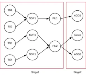
In this paper, we propose a method that extends the query optimization techniques presented in [1][2]. The method in [1] applies query re-optimization but considers only time while the method in [2] considers both time and monetary costs but does not employ query re-optimization. We combine the advantages of both. Our method is aimed to: (i) find a query execution plan which satisfies the user constraints, and (ii) reduce either the time cost or the monetary cost to execute a query. In our model, a QEP consists of a series of operators and these operators are divided into groups based on their dependencies and characteristics. The operators that can be executed on one container will be grouped together in one group which is called a Stage. Fig. 2 shows an example of a DAG generated by the query optimizer for the following query:
SELECT Department, count(Name) FROM STUDENT
GROUP BY Department WHERE Grade <=‘C’;
In this figure, TS, SOR, FIL and AGG stand for TableScan, Sort, Filter and Aggregate operators respectively. The subscripts distinguish the same operator that is executed in parallel on different data. And the arrows denote the dependencies between different operators. For example, AGG operators must wait for its previous operator, FIL to be finished.
A query execution schedule can be used to define the allocation of operators and containers, as well as the starting and ending time of execution. This kind of schedule is modeled as
= , , ,
where assign denotes an assignment of an operator to a
container. denotes the operator op in the i-th optimization;
denotes the container j; tstart and tend denote the start and
ending timestamps of the operator. The cost of a schedule is defined as
( ) = ,
which is a two-dimensional variable describing the amounts of time and money for the execution of a QEP. Similarly, the
constraint = , is also a
two-dimensional variable which describes the time and money cost requirements for the execution of a QEP. We say that
( ) if the costs of a schedule is equal
to or less than the user constraints on every dimension.
Similarly, ( ) ( ) denotes if
both time and monetary costs of Schedule A are less than the time and monetary costs of Schedule B.
We make the following assumptions: The containers are heterogeneous, i.e. containers have different CPU processing power and leasing price. The cost of a schedule will be varied as each schedule operator will be assigned to a different container and each container has a different CPU capacity and container configuration. If the accumulative CPU usage of all the operators in one container exceeds the capacity of the container, the estimated execution time of these operators will be multiplied by the CPU usage. Thus, the time of each schedule will be different depending on the container assignment. The monetary cost of the schedule will be changed accordingly. To find a schedule that satisfies the user constraints, a search optimization algorithm is needed which we will describe in the next section.
IV. ADAPTIVE QUERY EXECUTION OPTIMIZATION In our proposed method, a regular query optimizer first generates an initial QEP. Then this QEP will be divided into stages and executed by the execution engine stage by stage. After finishing each stage, the data statistics will be updated. These statistics include the cardinality, selectivity, max and min values for each attribute in each database table. By updating these statistics, the estimation of the resulting data size used in the next stages will be updated accordingly. The rest of the stages in the QEP are also sent to the query optimizer for re-optimization using the updated statistics. Three things are required to be submitted to the system by the user: the query, the
Figure 2. QEP is divided into different stages after being compiled from the query
time constraint, and the monetary cost constraint. Our adaptive optimization algorithm (AOPT) presented in Algorithm 1 is the main framework which gives an overview of how the query is processed. Algorithm 1 will call Algorithms 2 and 3. Algorithm 2 describes how the containers are assigned to execute the QEP and Algorithm 3 describes how each schedule is optimized individually.
As we can see in Algorithm 1, the user submits a query and the time and monetary cost constraints for finishing the query. In Line 1, the query is compiled into a query optimizer tree. This tree contains all the physical operators needed to process the query. Line 2 shows that these operators are grouped into different stages. The operators that do not required the results from their previous operators can be grouped together. In Line 3, the Optimizer_Tree is processed one stage at a time. In Line 4, a stage is mapped to a DAG according to their dependencies in the Optimizer_Tree. In Line 5, Algorithm 2 is called to generate an initial schedule which is optimized by Algorithm 3 in Line 6. The result is then obtained by executing all the operators in the current stage according to the Optimized_Schedule. The finished operators in the current stage are then eliminated from the Optimizer_Tree. The process from Line 3 to Line 10 is repeated for each stage until all the stages are finished and the final result is returned to the user. The following paragraph explains how to find an optimized schedule and illustrates the cost reducing re-optimization process of this
schedule. To better illustrate the idea, we provide a running example. Suppose we execute the query given in Section III, and the user constraints are as follows: the query response time must be less than 2 minutes, and the monetary cost must be less than $30. Assume that each container costs $0.1 per second. The database table STUDENT is stored in 3 separate locations. Each table has three columns, Name, Department and Grade, and each of the three tables contains 65,000 rows of data. The first step is converting the query to the optimized operator tree like in traditional database systems. The query optimizer groups these operators including TableScan, Filter, Sort, Aggregation, Merge, and Partition into different stages. For example, Stage 1 and Stage 2 are shown in Fig. 3.
After the stages are formed, the first operator TableScan will be executed on 3 data partitions in parallel on 3 different
Algorithm 1: ADAPTIVE OPTIMIZATION (AOPT) DESCRIPTION:
This is the main query processing algorithm which includes query optimization, query re-optimization, and query execution. INPUT:
Sql: query.
CONS: two-dimensional variable containing time and money constraints.
C: a set of containers each of which has the percentage of the current CPU usage and the network bandwidth.
P: unit price of leasing one container. Minimum value: a loop control parameter. Iteration-limit: a pre-defined variable. OUTPUT:
Result: the result of the query.
1. Ops <- compile query Sql to get its set of compiler-generated operators
2. Optimizer-Tree <- generate a multi-staged optimizer tree from the set of operators Ops
3. for each stage in the multi-staged Optimizer-Tree 4. G <- map the stage in Optimizer-Tree to form a
dataflow graph
5. Initial-Schedule <- call function DISPATCH(G, C, CONS) to assign operators to containers to form the initial schedule
6. Optimized-Schedule <- call function
OPTIMIZE(Initial-schedule, CONS, Minimum value, Iteration-limit, P) to find the optimized schedule for the initial schedule
7. Result <- execute the current stage of Optimized-Schedule
8. Optimizer-Tree <- Eliminate the finished operators from the Optimizer-Tree
9. Update constraints and data statistics 10. end for
11. return Result
Stage 1:
Table Scan: [Table=student.chunk1; estimate number of
rows=30,000; Data Size=300 KB]
Filter:[Column=student.grade; expression=‘>=C’ ;
estimate number of rows=30,000;Data Size=300 KB; cardinality=4; ]
Sort: [Column=student.department; estimate number
of rows=32,500; Data Size=32.5 KB; order=ascending]
Stage 2:
Aggregation:[expression=count(student.name);
estimate number of rows=32,500; Data Size=32.5 KB]
Partition: [key=STUDENT.Department ; cardinality=5;
estimate number of rows=5]
Merge: [expression=sum(count(STUDENT.Name)),
number of partition=5; estimate number of rows=5]
Output:
[Column=Department,count(STUDENT.Name), format=text]
Figure 3. A QEP compiled from the SQL query. This QEP contains stages, operators and the estimations of these operators.
containers and the allocation of containers is decided by the Algorithm 2. In Algorithm 2, the execution time of each operator executed on each container is first estimated. Then, from Line 6 to Line 9, a set of candidate containers are found for the next operator that has no dependencies. These candidate containers are the ones that the operation execution time estimate satisfies the user time constraint. From Line 13 to 19, this operator will be assigned to the container which has the shortest estimation time. This assignment is then added to the schedule with its current timestamp as the starting time. The current timestamp plus the estimating execution time is added as the ending time. This process keeps repeating until all the operators in the DAG have been assigned. Since this schedule is not optimized yet, it is called the initial schedule. One initial schedule looks like the following:
initial_schedule= { Assign( ,c1,12.3,75) Assign( ,c1,0,12.3) Assign( ,c2,0,65) Assign( ,c3,12.3,65) Assign( ,c1,75,75.05) Assign( ,c2,75,75.05) }
where Assign( ,c1,0,75) means the sort operator is
assigned to be executed on the container 1, the estimated starting time is 0 and the estimated ending time is 75. This initial schedule may not meet the constraints, so it will then be optimized by the simulation annealing algorithm [5] presented in Algorithm 3. This creates an optimized schedule which satisfies user constraints. The following is an example of an
optimized schedule. We can see that the assignment of is
changed from c1 to c3. optimized_schedule= { Assign( ,c1,12.3,75) Assign( ,c3,0,12.3) Assign( ,c2,0,65) Assign( ,c3,12.3,65) Assign( ,c1,75,75.05) Assign( ,c2,75,75.05) }
From the optimized schedule above, we obtain the estimated total time for executing the query as 75.05 as the last operator finished at 75.05 seconds and the monetary cost is calculated by each container cost $0.1 per second which is
$0.1
∗ (75.05 )(3 ) = $22.515
After the completion of a stage, the statistics are updated with the new statistics collected from the finished stage. The user's constraints will be adjusted to reflect the remaining constraints for the unfinished stages. Each new constraint is computed as follows:
New Constraint = Old Constraint − (Elapsed Cost + Overhead)
where the Elapsed Cost is the accumulated actual time and monetary cost of all the previously executed stages and the Overhead is the overhead of collecting the new statistics and updating the estimations. For example, after the execution of Stage 1, we update the constraints first as follows:
= 120 − (75.05 + 0.01 )
= 44.94
= $30 − ($22.515 + $0.003)
= $7.482
Then we update the operators in the unfinished stages with the new statistics gathered from the completed stages. For example, the actual data size after executing the FIL operators in Stage 1 is lower than the estimated data size before the query is executed. Then, the number of containers needed to execute the AGG operator in Stage 2 is reduced accordingly; otherwise, the number of containers used in Stage 2 is not updated and there will be some wasted containers. In our example, the number of containers needed to execute Stage 2 is reduced from 2 to 1. Thus, the total monetary cost is reduced. Using the same procedure, this AGG operator will still be sent to the scheduler to be optimized and executed.
Algorithm 2: DISPATCH [1] DESCRIPTION:
This algorithm assigns containers to the stages of QEP. INPUT:
G: the dataflow graph. C: a set of containers.
CONS: two-dimensional variable containing time and money constraints.
OUTPUT:
SG: Schedule with assignment of operators to container. 1. SG. assigns <- Ф
2. ready <- {operators in G has no dependencies} 3. for all operators in dataflow graph G
4. estimation_duration <- {estimate execution time of each operator}
5. end for
6. while ready != Ф do
7. n <- {Next operator to assign}
8. Candidates <- {containers that assignment of n 9. satisfy CONS}
10. if candidates = Ф then 11. return ERROR 12. else
13. C <- {the container which has minimum time cost if this operator run on this container}
14. assign(n,C) 15. ready <- ready - {n}
16. ready <- ready + {operator that have no dependencies}
17. start_time<- {current timestamp} 18. SG.assigns <- SG.assigns + {assign(n, c,
start_time, start_time+estimation_duration)} 19. end while
An optimized schedule of Stage 2 is:
optimized_schedule= {
Assign( ,c1,75.05,75.10) }
Suppose the time cost of finishing AGG operator is 0.05 sec. In the original schedule, the monetary cost of finishing Stage 2 is
(2 ) $0.1
∗ (0.05 ) = $0.01
and after the query re-optimization, even the time remains unchanged, but the monetary cost becomes
(1 ) $0.1
∗ (0.05 ) = $0.005
For this partial query, the monetary cost is halved. This will benefit the total time cost as well as the monetary cost of the whole query execution plan. Such savings are substantial considering the high number of queries issued in many real-world applications.
V. EXPERIMENT AND RESULT
A. Dataset and Configuration
We used 10 virtual machines to simulate the cloud environment. Each virtual machine had a 3.0Ghz single CPU and 2GB of RAM. A virtual machine is defined the same as the containers mentioned in the previous section.
A synthetic dataset was used and the maximum data size in the experiment is 1.9TB. One database table named PATIENT with the attributes pid, patient_firtname, patient_lastname,
birthday, and heart_rate is populated with varied volumes of
randomly generated data. Two different types of queries were executed on this table to test the impacts of query types on the performance of our algorithm. In the first query type, the query operator changed after reoptimization. In the second query type, the number of containers used to execute a query changed after reoptimization. These two types of queries are adopted from [2]. For each set of experiments, we ran 30 different query instances of the same type on each data size and averaged out the query response time and monetary costs.
B. The Impact of Data Size on Different Degrees of Parallelism
We hypothesize that query re-optimization is able to reduce the degree of parallelism of a query execution plan. This means the query response time and monetary cost will be reduced as fewer computational nodes are planned to be used.
The example Query 1 given below was executed to test whether the time cost or monetary cost will be affected by the query execution plan’s degree of parallelism [2]. This is because the number of containers used in the query execution will be influenced. In this query there are sub-queries that select data from different partitions of the table and are executed in parallel, so there is a high degree of parallelism in this query.
Query 1:
SELECT pid,RecursiveUDA(hr) AS sb FROM (SELECT pid, hr, FROM patient_1 UNION
Algorithm 3: OPTIMIZE (OPT) DESCRIPTION:
This algorithm optimizes a schedule using Simulation Annealing[8].
INPUT:
Initial_schedule: a schedule to be optimized.
Cons: a two-dimensional variable containing time and money constraints.
Minimum value: a loop control parameter. Iteration_limit: a pre-defined variable. P: unit price of leasing one container. OUTPUT:
SG: an optimized schedule with estimated time and money costs that satisfies the constraints
1. old_schedule <- Initial_schedule
2. old_cost <- GET_COST(old_schedule, P) 3. while T is greater than Minimum value 4. while i is less than Iteration_limit
5. new_schedule <- {find a neighbor schedule of old_schedule}
6. new_cost <- GET_COST(new_schedule, P) 7. if new_cost dominates old_cost and
new_cost satisfies Cons
8. {add the new_schedule to the schedule space} 9. old_schedule <- new_schedule
else
10. ap <- {calculate the acceptance probability with old_cost, new_cost and T}
11. if ap is greater than a multi-dimension value 12. in every dimension 13. old_schedule <- new_schedule 14. end if 15. end if 16. i++ 17. end while 18. reduce the value of T 19. end while
20. return SG <- {select a schedule from the schedule space}
FUNCTION: GET_COST (Schedule, P) INPUT:
Schedule: a schedule needs to be evaluated for the cost. P: unit price of leasing one container.
OUTPUT:
Cost: a two dimensional variable contains time and monetary costs of the input schedule.
1. Cost.time<- Ф 2. Cost.money<- Ф
3. for each assignment A in Schedule 4. if A.tend is the largest timestamp
5. Cost.time<-A.tend
6. end if
7. Cost.money<-Cost.money+(A.tend-A.tstart)*P
8. end for 9. return Cost
SELECT pid, hr, FROM patient_2 UNION
SELECT pid, hr, FROM patient_3 ) AS R
WHERE UDF(pid,hr)>80 GROUP BY pid
We purposely made the size of the intermediate data of execution extremely small after the User Defined Function (UDF) was performed. We expect to see that if re-optimization is applied, the new intermediate data size used in the remaining stages will result in a change of containers used accordingly. (shown in Table I). And evidently, the monetary cost will also change.
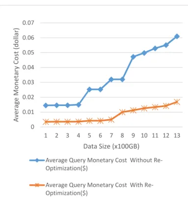
From Fig. 5, we can see that the monetary cost of query execution has been reduced with the re-optimization. However, the query response time does not notably change, only within an 8% difference, while the query monetary cost is reduced over
40% on average. This is because the degree of parallelism is updated after each stage; if the degree of parallelism is small, we will schedule fewer containers for the rest of the QEP execution. Thus, the monetary cost is reduced. For example, when the data size is over 1,000 GB, the peak number of containers needed without re-optimization is 8 but this number is reduced to 2 with re-optimization. As 6 fewer containers are used in query execution, this saves monetary cost.
C. The Impact of Data Size on Different Physical Operators
In this experiment, we studied the impact of physical operators and the impact of different data sizes on these physical operators. Physical operators will be changed with different data statistics even with the same logical operators in the QEP. Similarly, if the QEP is not re-optimized, this change will not be detected before the query is actually executed and the statistics are updated. To reflect this change, we changed the type of the Join operator during the query execution. To test its impact, we ran the following Query 2 [2]:
Query 2:
SELECT R.p_id,R.p_name,R.sc,S.p_hr
FROM (SELECT p_id, p_name, AVG(p_bp) AS sc FROM patient GROUP BY p_id,p_name) AS R JOIN (SELECT p_id,p_hr
FROM patient
WHERE UDF(p_id,p_hr)>80 ) AS S
ON R.p_id=S.p_id
Figure 5. Impact of data size on monetary cost for execution of Query 1.
0 0.01 0.02 0.03 0.04 0.05 0.06 0.07 1 2 3 4 5 6 7 8 9 10 11 12 13 Avera ge Mo n et ary Co st (d o lla r) Data Size (x100GB)
Average Query Monetary Cost Without Re-Optimization($)
Average Query Monetary Cost With Re-Optimization($)
Figure 4. Impact of data size on query response time of Query 1
0 20 40 60 80 100 120 140 160 180 1 3 5 7 9 11 13 15 17 19 Avera ge Q u ery Resp o n se Time (seco n d ) Data Size (x100GB)
Average Query Response Time Without Re-Optimization(sec)
Average Query Response Time With Re-Optimization(sec)
TABLEI.THECOMPARISONOFPEAKNUMBEROFCONTAINERS USEDINEXECUTIONOFQUERY1
Data Size (x100GB) Peak number of Containers used without Re-optimization Peak number of Containers used with Re-optimization 1 4 2 5 4 2 10 8 2 15 8 2 20 8 2
In this query, there is a Join of two subqueries. The data size of each subquery is unknown. We want to see how the physical operator of this Join will change depending on the data size of the subquery. So, we purposely made the data size of the right side of the Join operator small enough to fit in the cache. As a consequence, the Shuffle Join operator will be changed to the Broadcast Join operator for every query execution.
As seen from Fig. 6, when the physical operator of Join was changed from Shuffle Join to Broadcast Join, the execution time was reduced. This is because the BroadCast Join is executed around 40% faster than Shuffle Join in this environment. The overall time cost using re-optimization
has a rough 20% improvement average over no re-optimization. Also, as shown in Fig. 7, the bigger the data size, the more time was saved with re-optimization as opposed to without re-optimization. This is despite the fact that both approaches will require more time for query execution. The results show that re-optimization is valuable for large data size. The monetary cost between the two approaches was close, with only a 4% difference as shown in Fig. 8. This divergence in monetary cost occurs when some part of the query is executed on the containers with higher unit price after re-optimization.
V. CONCLUSION AND FUTURERESEARCH
In this paper, we proposed a method that adaptively optimizes a query execution plan to satisfy both the query response time and monetary cost objectives. A query is first converted to a multi-staged query execution plan. Then, after the completion of each stage, the query execution plan is adjusted with the new database statistics to reduce the time and monetary costs. This is done until all the stages are finished and the final query result is obtained. Our experimental results show that query re-optimization is able to improve either the time cost or the monetary cost depending on the type of queries to be executed. If the queries need a high degree of parallelism, then the monetary cost can be reduced (see Fig. 5 and Table I). If the queries contain different Join physical operators after query re-optimization, then the time cost can be reduced.
Our results show that after query re-optimization, either the query response time or the monetary cost benefits from our algorithm. For executing queries using query re-optimization on different containers like Query 1 in Section IV, the query response time is 20% less than the query response time without optimization. Although, the monetary cost before and after re-optimization remains similar, with only a 5% difference. For queries that have operators changed during query re-optimization like Query 2 in Section IV, the monetary cost is
0 5 10 15 20 25 30 35 40 45 50
Response Time (sec) Monetary Cost (x $0.001)
Shuffle Join without Re-optimization BroadCast Join with Re-optimization
Figure 7. Impacts of Data Size on Time for Executing Query 2.
0 10 20 30 40 50 60 70 1 2 3 4 5 6 7 8 9 10 11 12 13 14 15 16 17 18 Avera ge Q u ery Resp o n se Time (seco n d ) Data Size (x100GB)
Average Query Response Time Without Re-Optimization(sec)
Average Query Response Time With Re-Optimization(sec)
Figure 8. Impacts of data size on monetary cost for executing Query 2.
0 0.005 0.01 0.015 0.02 0.025 0.03 0.035 0.04 0.045 0.05 1 2 3 4 5 6 7 8 9 10 11 12 13 14 15 16 17 18 Avera ge Mo n et ary Co st (d o lla r) Data Size (x100GB)
Average Query Monetary Cost Without Re-Optimization($)
Average Query Monetary Cost With Re-Optimization($)
Figure 6. Impact of physical operators on time and monetary cost for execution of Query 2.
roughly four times less than without using re-optimization, while the query response time is almost the same in both techniques.
As query re-optimization has notable overhead, we plan in our future work to develop methods for determining when to re-optimize. This is so we can avoid unnecessary re-optimization, that is, re-optimization that does not improve query execution costs. We plan to use machine learning algorithms to predict when to re-optimize queries so that the re-optimization will gain on time cost and/or monetary cost.
ACKNOWLEDGMENT
This work is partially supported by the National Science Foundation Award No. 1349285.
REFERENCES
[1] H.Kllapi, E.Sitaridi, M.Tsangaris, and Y.Ioannidis, "Schedule optimization for data processing flows on the cloud," Proc. 2011 ACM SIGMOD International Conference on Management of data (SIGMOD '11).2011, pp. 289-300. DOI: https://doi.org/10.1145/1989323.1989355
[2] N.Bruno, S.Jain, and J.Zhou, "Continuous cloud-scale query optimization and processing, " Proc. VLDB Endow. 6, 11, August 2013, pp. 961-972. DOI: http://dx.doi.org/10.14778/2536222.2536223
[3] A.Meister, S.Breß, and G.Saake, "Cost-aware query optimization during cloud-based Complex Event Processing," Lecture Notes in Informatics (LNI), Proceedings - Series of the Gesellschaft Fur Informatik (GI), P-232, pp. 705–716.
[4] N.Robinson, S. A.McIlraith, and D.Toman "Cost-based query optimization via AI planning," Proc. the National Conference on Artificial Intelligence, 3, pp.2344–2351.
[5] Z.Karampaglis, et al. "A Bi-objective Cost Model for Database Queries in a Multi-cloud Environment," Proc. the 6th International Conference on Management of Emergent Digital EcoSystems. (MEDES '14), 2014,Buraidah, Al Qassim, Saudi Arabia, pp.109-116.
[6] C. M.Costa, and A.L.Sousa, "Adaptive Query Processing in Cloud Database Systems," Proc. 2013 International Conference on Cloud and Green Computing, Karlsruhe, Germany, September 30 - October 2, 2013 pp. 201–202, IEEE Computer Society.
[7] D.Stamatakis, and O.Papaemmanouil,"SLA-driven workload management for cloud databases," Proc. 30th International Conference on Data Engineering Workshops, (ICDE 2014), Chicago, IL, USA, March 31 - April 4, 2014,pp. 178–181, IEEE Computer Society.
[8] S.Kirkpatrick, C. D. Gelatt, and M. P. Vecchi. "Optimization By Simulated Annealing". Science 220.4598, 1983, pp 671-680.
[9] Y. Gao, Yanzhi Wang, S. K. Gupta and M. Pedram, "An energy and deadline aware resource provisioning, scheduling and optimization framework for cloud systems," 2013 International Conference on
Hardware/Software Codesign and System Synthesis (CODES+ISSS), Montreal,QC,2013,pp.1-10.doi: 10.1109/CODES-ISSS.2013.6659018 [10] I. Abdelaziz, E. Mansour, M. Ouzzani, A. Aboulnaga and P. Kalnis,
"Query Optimizations over Decentralized RDF Graphs," 2017 IEEE 33rd International Conference on Data Engineering (ICDE), San Diego, CA, 2017,pp.139-142.doi: 10.1109/ICDE.2017.59
[11] T. Mastelic, A. Oleksiak, H. Claussen, I. Brandic, J. Pierson and A. Vasilakos, "Cloud Computing", CSUR, vol. 47, no. 2, pp. 1-36, 2014. [12] Z. Abul-Basher, "Multiple-Query Optimization of Regular Path
Queries," 2017 IEEE 33rd International Conference on Data Engineering (ICDE), San Diego, CA, 2017, pp.1426-1430. doi: 10.1109/ICDE.2017.205
[13] W.Wu, J. F Naughton, and H. Singh, "Sampling-Based Query Re-Optimization, " Proc. 2016 International Conference on Management of Data (SIGMOD'16).pp.1721-1736.
DOI:https://doi.org/10.1145/2882903.2882914
[14] R.Marcus and O.Papaemmanouil, "WiSeDB: A Learning-based Workload Management Advisor for Cloud Databases," Proc. VLDB Endowment. 9. 10.14778/2977797.2977804, 2016
[15] S.Soltesz et al. "Container-Based Operating System Virtualization", Proc. the 2nd ACM SIGOPS/EuroSys European Conference on Computer Systems 2007 (EuroSys '07), 2007.
[16] M. G. Xavier, M. V. Neves, F. D. Rossi, T. C. Ferreto, T. Lange and C. A. F. De Rose, "Performance Evaluation of Container-Based Virtualization for High Performance Computing Environments," 2013 21st Euromicro International Conference on Parallel, Distributed, and Network-Based Processing,Belfast,2013, pp.233-240.doi: 10.1109/PDP.2013.41
[17] R. Graham, "Bounds for Certain Multiprocessing Anomalies", Bell System Technical Journal, vol. 45, no. 9, pp. 1563-1581, 1966.
[18] B. Malakooti,"Operations and production systems with multiple objectives,", Wiley, Feb 2014
[19] M. Liu, Z. Ives and B. Loo, "Enabling Incremental Query Re-Optimization", Proc. 2016 International Conference on Management of Data (SIGMOD'16), 2016, pp.1705-1720.
DOI: https://doi.org/10.1145/2882903.2915212
[20] F. Helff, L. Gruenwald and L. d'Orazio, "Weighted Sum Model for Multi-Objective Query Optimization for Mobile-Cloud Database Environments," in Proceedings of the Workshops of the EDBT/ICDT 2016 Joint Conference EDBT/ICDT 2016, Bordeaux, France, 2016.
[21] S.Hiroyuki, M.Minami, and T.Keiki, "An improved MOEA/D utilizing variation angles for multi-objective optimization," Proc. the Genetic and Evolutionary Computation Conference Companion (GECCO '17). ACM, New York, NY, USA, 2017,pp.163-164.
DOI: https://doi.org/10.1145/3067695.3076037
[22] G.Abhinav, and D.Kalyanmoy, "Adaptive Use of Innovization Principles for a Faster Convergence of Evolutionary Multi-Objective Optimization Algorithms," Proc.the 2016 on Genetic and Evolutionary Computation Conference Companion (GECCO '16 Companion), Tobias Friedrich (Ed.). ACM, New York, NY, USA, 2016, pp.75-76.
DOI: https://doi.org/10.1145/2908961.2909019
[23] Amazon, Amazon EC2 Pricing, 2015. [Online].Available: https://aws.amazon.com/ec2/pricing/?nc1=h_ls. [Zugriff am 18 08 2015].