HAL Id: hal-02391242
https://hal.archives-ouvertes.fr/hal-02391242v2
Submitted on 10 Dec 2019
HAL is a multi-disciplinary open access
archive for the deposit and dissemination of
sci-entific research documents, whether they are
pub-lished or not. The documents may come from
teaching and research institutions in France or
abroad, or from public or private research centers.
L’archive ouverte pluridisciplinaire HAL, est
destinée au dépôt et à la diffusion de documents
scientifiques de niveau recherche, publiés ou non,
émanant des établissements d’enseignement et de
recherche français ou étrangers, des laboratoires
publics ou privés.
Resource allocation for edge computing with multiple
tenant configurations
Andrea Araldo, Alessandro Stefano, Antonella Stefano
To cite this version:
Andrea Araldo, Alessandro Stefano, Antonella Stefano. Resource allocation for edge computing with
multiple tenant configurations. SAC 2020: 35th Symposium On Applied Computing, Mar 2020, Brno,
Czech Republic. pp.1190-1199, �10.1145/3341105.3374026�. �hal-02391242v2�
Resource Allocation for Edge Computing with Multiple Tenant
Configurations
Andrea Araldo
Télécom SudParis Institut Polytechnique de ParisFrance
andrea.araldo@telecom- sudparis.eu
Alessandro Di Stefano
University of Catania Department of Electrical, Electronicand Information engineering Italy
Antonella Di Stefano
University of Catania Department of Electrical, Electronicand Information engineering Italy
ABSTRACT
Edge Computing (EC) consists in deploying computational resources,
e.g., memory, CP Us, at the Edge of the network, e.g., base stations, access points, and run there a part of the computation currently
running on the Cloud. This approach promises to reduce latency, inter-domain traffic and enhance user experience. Since resources at the Edge are scarce, resource allocation is crucial for EC. While
most of the studies assume users interact directly with the Edge submitting a sequence of tasks, we instead consider that users will
interact with different Service Providers (SPs), as they currently do in the Web. We therefore consider the case of a Network Operator
(NO) that owns the resources at the Edge and must decide how much resource to allocate to the different tenants (SPs).
We propose MORA, a polynomial time strategy which allows the NO to maximize its utility, which can be inter-domain traffic savings, improved users’ QoE or other metrics of interest. The core
of MORA is that (i) it exploitsservice elasticity, i.e., the fact that
services can adapt to the resources allocated by the NO and rely on
a remote Cloud for the excess of computation, (ii) it is suitable for micro-services architecture, which decomposes a single service in a set of components, which MORA places in the different
computa-tional nodes of the Edge and (iii) it copes withmulti-dimensional
resources, e.g., memory and CPUs. After analyzing the properties of the algorithm, we show numerically that it performs close to the optimum. To guarantee reproducibility, the numerical evaluation is
performed on publicly available traces from Google and Alibaba clusters and in synthetic scenarios and our code is open source.
CCS CONCEPTS
•Networks → Cloud computing; Network management;
Pro-grammable networks; • Computer systems organization → Cloud computing; n-tier architectures;
Permission to make digital or hard copies of all or part of this work for personal or classroom use is granted without fee provided that copies are not made or distributed for profit or commercial advantage and that copies bear this notice and the full citation on the first page. Copyrights for components of this work owned by others than the author(s) must be honored. Abstracting with credit is permitted. To copy otherwise, or republish, to post on servers or to redistribute to lists, requires prior specific permission and /or a fee. Request permissions from [email protected].
SAC ’20, March 30-April 3, 2020, Brno, Czech Republic
© 2020 Copyright held by the owner/author(s). Publication rights licensed to ACM. ACM ISBN 978-1-4503-6866-7/20/03. . . $15.00
https://doi.org/10.1145/3341105.3374026
KEYWORDS
Cloud Computing, Edge Computing, Resource allocation, Container
systems, Network optimization
ACM Reference Format:
Andrea Araldo, Alessandro Di Stefano, and Antonella Di Stefano. 2020.
Re-source Allocation for Edge Computing with Multiple Tenant Configurations.
InThe 35th ACM/SIGAPP Symposium on Applied Computing (SAC ’20), March
30-April 3, 2020, Brno, Czech Republic. ACM, New York, NY, USA, 10 pages. https://doi.org/10.1145/3341105.3374026
1
INTRODUCTION
Under the paradigm of Edge Computing (EC), computational
ca-pabilities, e.g., memory and processing elements, are deployed di-rectly in the access networks, close to the users. This enables low
latency applications, reduces the traffic going out from the access networks and can improve user experience. EC is complementary to
Cloud [30]. In the Cloud, resources are usually assumedelastic, i.e.,
they are always available, as long the third party Service Provider (SP) is willing to pay. On the contrary, contention emerges in the
Edge between SPs sharing limited resources and the problem arises of how to allocate them between SPs.
The problem we solve in this work is the one of a Network Op-erator (NO), owning limited computational resources in its Edge
network, which must decide how to distribute them to different SPs. The goal of the NO is to maximize its own utility, which can
repre-sent bandwidth or operational cost saving or improved experience for his users [7, 15].
The core of our approach is that we exploitservice elasticity: a
service can run at the Edge under different configurations. Today, these scenarios are common in services as video streaming, in which
the SP has to deliver different encodings of the same video and can choose whether to pre-package all these representations and store
them, which requires a high amount of memory. Alternatively, with Just In Time Packaging ( JITP) SPs can store just few representations
and package the missing ones on-the-fly, only when needed, which saves memory space but incurs more CP U usage [15]. In the Edge, we do not have resource elasticity as in the Cloud, but at least we
can exploit service elasticity, which is the aim of MORA. We show that, by doing so, the NO can increase its utility with respect to the
classical case of one monolithic configuration per SP.
Furthermore, we consider the distributed nature of Edge
re-sources, which can be scattered across different nodes and the fact that services follow a microservice architectural style (Sec. V.B of [26]): a service is composed of different microservices running
oncontainers. This allows fine-grained and responsive service adap-tivity and resource exploitation, which makes containers attractive for Edge computing [12].
Another important aspect of MORA is its polynomial time effi-ciency. Since user demand is expected to change in fast time-scales
and so are the resources required by the SPs, the allocation must be calculated ideally within few seconds. For example, a Content Delivery Network usually recalculates the association between
de-mand and computing nodes every 10 to 30 seconds [22]. Some work assumes even higher re-allocation frequency [30].
The paper is organized as follows: §2 discuss the related work; §3 describes the architecture we have in mind; §4 reports an
Inte-ger Linear Programming (ILP) formulation of the multiple-tenant multiple-configuration allocation problem; §5 describes MORA, its
computational complexity and gives a bound to the optimal so-lution; §6 reports the numerical results on synthetic data and on publicly available traces.
2
RELATED WORK
We study the case of Metro Edge Cloud and Mobile Edge Comput-ing [12, 27], in which there are computation nodes concentrated
in small data-centers located into the Network Operator Central Office (CO) or co-located in the base station. While there is vast
literature on EC [12, 26, 27], we focus in this section just on work concerning resource allocation. We survey applications of this prob-lem on EC and also on completely different domains, if the applied
methodology gives useful insight for our problem. To the best of our knowledge no previous work has attempted to exploit service
elasticity (§ 1), which we show instead in this paper to improve resource exploitation in a resource constrained environment like
EC. This is, we think, the main merit of our work.
2.1
Resource allocation for container-based EC
The problem of containers resource allocation has been investigated
using time-slicing [25], Fuzzy [29], linear programming models [32], reinforcement learning [24]. Others authors also employ non-standard techniques like vertical elasticity [5]. Most work considers
only a single type of resource to allocate, i.e., CP U [25], with few exceptions [24, 29]. Some work considers all resources aggregated
in one single pool [24], while others [5, 29] consider that they are distributed across different nodes, which complicates the allocation
problem. The objective is generally to minimize network traffic, energy [32] or execution time [24].
As for the information to support the allocation decision, most
work is based on a “monitor-and-decide” approach [5, 24, 29], but it is becoming common to also use detailed information on the
workloads by the users [4, 11, 29]. When implementing allocation strategies, a Docker scheduler [5, 25] is mostly assumed.
2.2
Edge-Cloud hierarchy
EC is complementary to Cloud, i.e., the usual assumption is that a part of service computation is peformed at the Edge and the rest on
the Cloud and similarly a part of the required data seats at the Edge and the rest on the Cloud. In a sense, the Edge-Cloud infrastructure is hierarchical [13, 23, 30], where Edge resources are the leaves
and the upper nodes are Cloud clusters. In [30] the decision of
how much capacity must be provisioned across the levels of the
hierarchy. Similar to our proposal, workloads have requirements and can fit into a node if its capacity is not violated, but resources
are mono-dimensional. A similar problem is tackled by [23], but nodes are modeled as queues and CP U and network traffic are
jointly considered. Queueing models are also employed in [13], which focuses on load balancing between Edge and Cloud. The set up all this work is different from ours, as they do not consider
contention between multiple tenants, i.e., the SPs of our set up.
2.3
Other resource allocation problems
Game theory is used to allocate resources between tasks submitted by users [16]. In our work, instead, contention does not emerge between user tasks, but between third party services. Recent
litera-ture exists on cache allocation, in which the NO allocates memory to third party SPs to minimize bandwidth consumption [7] or QoS
and fairness [10] (CP U is ignored). Similar to our proposal, but in a simpler context, the tasks modeled in [20] can run in different
configurations, each using a different combination of resources and resulting in a different perceived utility for the users. Their model explicitly represent the relation between resource usage, an
indication of the “quality” achieved and some “utility”. However, in their numerical experiments simulation input datas are randomly
generated. We thus preferred to associate a certain resource usage to a utility for the Network Operator directly, assuming this
rela-tion can be obtained by measurements (of bandwidth consumed, of users’ QoE [9]). Moreover, [20] do not consider multiple-servers and
multiple-containers. Authors of [31] assume users send a sequence of tasks and each can run under different configurations, requiring a combination of different resource types. They assume users want
to run as many tasks as possible and their utility is number of tasks run. While this task-centric vision is more suitable for Grid-like
environments, we instead adopt the assumption services and users behave like in current applications in the web environment: instead
of submitting task, users instantiate connections with services and use them along a span of time. Therefore, while in [31] resources are consumed every time a task is submitted, we instead assume,
as in current Internet services, that resource consumption is not tight to the single task submitted. Take, for example, the case of
a video streaming service which requires memory to cache the most popular videos: memory is consumed in a "persistent" way,
i.e., independent of the single task submitted by users. We assume however that SP declares the resources needed based on its
pre-dicted demand. To summarize, differently from [31], our resource consumption does not come from single user’s tasks, but from the needs of SPs. Furthermore, utility is not the one of users, but the
one of the NO. Therefore, while [31] maximize the user utility or the product of users’ utility, we maximize instead the NO utility, as
the NO invested for Edge resources and wants to capitalize them. As a consequence, our problem is different and requires a different
strategy.
3
ARCHITECTURE AND INTERACTIONS
3.1
Limits of current architectures
Edge Computing is already being employed by big players in the Internet. As an example, Netflix deploys its own hardware, called
Resource Allocation for Edge Computing with Multiple Tenant Configurations SAC ’20, March 30-April 3, 2020, Brno, Czech Republic DeploymentFile = =Option =SP Proxy =Edge Node reque st request MORA Algorithm Edge Master decis
ion decisio
n deploys Edge Cloud Cloud 1 1 2 3 3 4 5 5 6 6 7 7 =Container SP1 SP2
Figure 1: Architecture of MORA .
Open Connect Appliances (OCAs) [3], into Internet access networks
and serves a fraction of users’ traffic directly from there. This gener-ates a utility to the NO, in terms of inter-domain traffic saving. On the other hand, Netflix has all its business assets (content and user
information) in its boxes and does not need to share it with NOs.
The limit of this solution is its limitedpermeability: it is unfeasible
in terms of cost and physical space to install hardware appliances to the very edge of the network, i.e., in many base stations, central
offices, access points, etc. Moreover, many other SPs, in addition to Netflix, would benefit from having their hardware installed in access networks, but it would be impractical for NOs to install them
all. Furthermore, SPs with less bargaining power than Netflix would have no strength to convince NOs to deploy their hardware
appli-ances. These limits can be overcome if appliances are virtualized, as it is already done in Cloud environments. We thus propose that
an NO deploys computational resources at the edge, e.g., memory and processing units, and then allocates slices of them to several
third party SPs. The SP can then use its assigned slice as it were a dedicated hardware. Memory encryption technologies [8] can guarantee that data and processing remain inaccessible to the NO,
even if they run in its premises. The problem we investigate in this paper is how to allocate resources to each SP in this setting.
Note that, while big players may continue to use their hardware appliances, our virtualized solution is probably the only way small
or medium SPs can reach the Edge of the network.
3.2
MORA architecture
The goal of MORA algorithm is to choose, for each SP, one of the
possible configuration options in which the service can run at the edge. We show here how our framework could be deployed in Edge
Computing. The entities and the interactions taking place periodi-cally, i.e., every 5 minutes, between them are depicted in Fig.1. Edge
resources are handled by anEdge Master, e.g., a Kubernetes Master,
managed by the NO. OneSP Proxy runs for each SP, which sends 1○
a request to the Edge Master, similar to Kubernetes Deployment
files. A request reports different configuration options at which the SP can run its service at the Edge. In particular, an option is a set of
containers. Therefore, in the request the requirements, e.g. memory and CP U, of all containers are reported. The request also reports the utility associated to each option, e.g., the bandwidth saved by
that configuration option with respect to the case where the SP has no containers running at the Edge. The Edge Master collects
the requests from the different SPs; runs MORA algorithm○ to2
Table 1: Summary of the notation.
Parameters
M Number of nodes
N Number of service providers
Ji Number of options by SPi
Zi, j Number of containers for optionj of SP i
cl,m Amount of resourcel in node m
wl,zi, j Amount of resourcel required by the container z of
optionj by SP i
ui, j Utility given by choosing optionj of SP i
Decision variables
xi, j Binary variable, 1 if the optionj by SP i is chosen, 0
otherwise
yz,mi, j
Binary variable, 1 if the containerz of option j by SP i
runs on nodem, 0 otherwise
select an option for each SP; communicates○ the decision to all3
SP Proxies; and deploys○ the containers of the chosen options,4
using the appropriate container images, pre-stored in a repository.
Connections from users to a certain SP are intercepted○ by the SP5
Proxy [21], which decides whether to associate users locally to the
Edge○, if the resources of the deployed containers are sufficient.6
Otherwise, the users are associated to a remote Cloud○, similarly7
to [13].
4
SYSTEM MODEL
We consider the case of a Network Operator (NO) owning an Edge
Computing infrastructure, composed ofm = 1, . . . , M nodes.
Re-sources are of typel = 1, . . . , L. In the numerical results we will
considerL = 2 resource types, namely memory and processing,
which are considered by modern orchestration frameworks as
Ku-bernetes.1Each nodem has a capacity cl,m, which is the amount of
resource of typel available. We have i = 1, . . . , N services
compet-ing to use the resources available at the edge. Similar to [14], we
consider that there is no unique way to run a service at the edge. If abundant resources are available, a service can be configured in
order to exploit them all, thus almost completely running at the edge. If less resources are available, the service may configure itself so to adapt to those and to move some of the computation and data
to some remote servers or cloud computing infrastructures (§ 1). We represent this possibility by specifying different configurations
(oroptions)j = 0, 1, . . . , Ji for the same service. In short we will
denote withij the j-th option of service provider i. We assume
services are “containerized” [26]. Therefore, each configurationj
is composed of a set of containersz = 1, . . . , Zi, j, each of which
requireswi, j
l,zunits of resource typel. The multiple configurations
in which a Service Provider (SP) can run its service at the edge denotes its capability to adapt to different amounts of resources
available. Each configuration results in a certain utilityui,z for
the Network Operator (NO), which in the simplest case represent bandwidth saving [7], which is what we consider in our results with
Alibaba cluster traces. Utility can in genral be cost savings [15],
1
QoS or fairness [10], elaboration time savings [16], depending on
the application and the information available. As commonly done in the literature [10, 15, 17], we adopt a “snapshot” approach by
assuming that the resources needed for the configurations and the other characteristics of the configurations are known at the moment
of taking the resource allocation decision. In our case, we assume they are declared by the SP itself, which is the only one knowing exactly the algorithms and the data involved in its computation.
This is in line with today containerized environments. For example, in Kubernates it is possible to define memory, CP U and bandwidth
limits when Deployment files are submitted. As commonly done in the literature [17, 22] we assume that there are mechanisms able to
provide good estimates of resources and utility, which fall outside the scope of this paper. Note also that we do not consider the cost of
instantiating and realising containers, since the snapshot approach cannot capture this kind of dynamics. We plan to fill this gap in future work.
The decision of the NO about which option from each SP should be accepted in the Edge and where to place the correspondent
con-tainers can be formulated in the following Integer Linear Program (ILP) as proposed in a previous work [6]. The binary decisions
vari-able arexi, j, which is 1 if thej-th option of the SP i is chosen, and
yi, jz,m, which is 1 if thez-th container of the j-th option of SP i is
placed on nodem.
The symbols used in the paper are reported in table 1.
max N ∑ i=1 Ni ∑ j=1 ui, j⋅ xi, j (1) s .t . M ∑ m=1 yz,mi, j =xi, j i = 1 . . . N j = 1 . . . Ji z = 1 . . . Zi, j (2) N ∑ i=1 Ji ∑ j=1 Zi, j ∑ z=1 yz,mi, j ⋅ wi, jl,z≤cl,m l = 1 . . . L m = 1 . . . M (3) Ji ∑ j=1 xi, j≤ 1 i = 1 . . . N (4) xi, j, yz,mi, j ∈{0, 1} i = 1 . . . N j = 1 . . . Ji z = 1 . . . Zi, j m = 1 . . . M (5)
The objective is to maximize the utility (1), setting the binary
variablesxi, j. Constraints (2) guarantee that each containerz of
the chosen optionj of SP i (xi, j = 1) is deployed (∃m ∈ {1 . . . M} ∶
yi, jz,m = 1). Constraints (3) guarantee that the sum of the
require-ments for the set of containers deployed on the same nodem for
each resourcel is less than the total amount of available resources
in nodem so that these containers can actually run on the node.
Finally, constraints (4) ensure that a SP can deploy at most one option in the Edge cluster.
Proposition 1. Problem P is NP-hard.
Proof. P reduces to a Knapsack Problem withL = 1, M = 1, Ji =
1, i = 1, . . . , N and Zi, j = 1, i = 1, . . . , N ; j = 1, . . . , Ji, which is
NP-hard. □
Reducing to 1 some of the dimensionsL, M, Ji, Z, we can reduce
the problem to Set-union Knapsack, Multiple-Choice Knapsack or Knapsack Problems. Our problem is complex and we rule out
the possibility to construct Fully Polynomial Time Approximation Schemes, as §9.4.1 of [18] shows that they cannot exist (unless
P=NP), already for the simpler case ofM = 1, Zi, j = 1 andJi =
1, i = 1, . . . , N , which is known as l-KP. All we can do is then to
propose a heuristic and show it is close to the optimum numerically.
5
MORA
We now introduce MORA, our proposed strategy.
5.1
Preliminary definitions
The MORA heuristic uses aggregate values for the resource
re-quirements and availability, in order to neglect, at a first stage, the complexity represented by the fact that resources available are
scat-tered across different nodes, resource required are split in different container requirements and requirements are multi-dimensional.
To this aim, we need to define the overall resource requirements
of an optionj of a SP i as wli, j= Zi, j ∑ z=1 wi, jl,z. (6)
We introduce a numberhl ≥ 0, that we call “relevance value”, since
its role is similar to the relevance values in §9.5.1 of [18]. We also
define the generalized resource utilization of an optionj of a SP i
as: wi, j= L ∑ l =1 hl⋅ wli, j (7)
To ease computation, MORA heuristic algorithm does not consider
all the possible options, but it first removes thedominated options
and thenLP-dominated options, defined as follows, which do not
provide significant utility gain with respect to the resources they require.
Definition 1. For any SPi, an option j is dominated by another
optionj′ ≠j iff (i) ui, j
′
>ui, jandwi, j′ ≤wi, j or (ii)ui, j′ ≥ui, j
andwi, j′<wi, j. An option is dominated, if it is dominated by some
other option.
Before giving the definition of LP-dominance, we need to define
theefficiency of a jump as follows.
Definition 2. For a service provideri = 1, . . . , N , the efficiency
of a jumpj → j′, wherewi, j′>wi, j is:
ei, j→j′= u i, j′ − ui, j wi, j′ − wi, j (8)
Definition 3. A non dominated optionj of a SP i is LP-dominated,
if there exist other non dominated optionsj′, j′′such thatui, j′<ui, j<
ui, j′′,wi, j′<wi, j <wi, j
′′
andei, j′→j′′ ≥ei, j
′→j
The optionj is an
LP-extreme if it is neither dominated nor LP-dominated.
The names “LP-dominance” and “LP-extremes” come from the fact that the concept is related to the LP-relaxation of the Mutliple
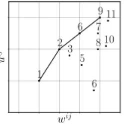
Resource Allocation for Edge Computing with Multiple Tenant Configurations SAC ’20, March 30-April 3, 2020, Brno, Czech Republic wij u ij 1 2 6 9 3 5 6 8 7 10 11
Figure 2: Example of set of options of a SPi. The options
con-nected by the line constitute the ordered list of LP-extremes.
Fig. 2 illustrates the concept of LP-extremes, similarly to Fig. 11.1 of [18]. We order the LP-extreme options in the list defined as
follows.
Definition 4. For each SPi, we denote with jithe list of its
LP-extreme options. We denote withji[k] the option at its k-th position.
This list is ordered in increasing values ofwi, j, such thatwi, j
i[k]
≤ wi, ji[k+1]. In the first position of such list we add a fictitious “null”
option, such thatwi, j
i[0]
=ui, j
i[0]
≜ 0.
Proposition 2. For any SPi, the list ji of LP-extremes can be
computed inO(∣Ji∣ ⋅ Ri), where Ri is the number of LP-extremes.
Proof. Ch. 11 of [18] shows that LP-extremes correspond to
the convex hull of the set of optionsj = 1, . . . , Ji. To compute the
convex hull we use [19], which has the complexity above. □
5.2
MORA Algorithm
The Multiple Option Resource Allocation (MORA) algorithm is shown in Algorithm 1. It takes as input the set of parameters of the ILP (9)-(4) describing the scenario plus a configuration parameter
hl forl = 1, . . . , L. The algorithm returns a solution, i.e. values for
any decision variable. The algorithm solves two decision problems
that the NO must solve: (i)Option selection: which option (or
config-uration) per SP must be accepted (variablesyz,mi, j ) and (ii)Container
placement: in which Edge nodes we should place the containers of
the selected options (variablesyi, jz,m). The pseudo code of Alg. 1 is
mainly devoted to option selection and calls Alg. 2 for the container
placement.
5.2.1 Option selection. MORA is iterative. In each iteration,
each SPi has a current position ki, which corresponds to the
op-tionji[ki]. Each SP i has also a jump efficiency Ei(line 6), which
denotes the efficiency achieved when advancing its position, i.e.,
the utility gain obtained going from optionji[ki] to ji[ki+ 1]
di-vided by the additional generalized resource utilized. Observe that
ui, ji[k] < ui, j i[k+1] andwi, j i[k] < wi, j i[k+1] by construction, and thusEi > 0.
Then, in each iterationt, we select a SP and we check whether
we can change its current optionji[ki] to ji[ki+ 1]. We say that
service provideri performs a jump ji[ki] → ji[ki + 1]. As one
can expect, we select the SP whose jump efficiency is the highest
(line 12). We call this SP thejumping SP of iterationt, as it is
the one that changes option (the options of the other SPs remain
unchanged).
We then try to place the containers of the jumping SPi∗(line 13).
If we succeed, we advance its current option, thus allowingi∗to
jump fromji
∗
[ki∗] to ji∗[ki∗+ 1] (line 15). Otherwise, we remove
the optionji
∗
[ki∗+ 1] that we have not been able to place. We
update the jump efficiency ofi∗.
The algorithm terminates when the listsjiof all the SPs have
been visited (line 10).
5.2.2 Container placement. The placement operations are
de-scribed in Alg. 2. We will refer toplacement as a mapping of a
container to an edge node. The algorithm works by constructing
atentative placement ˆyz,mi, j , ∀i, j, z,m. If we are able to construct a
feasible tentative placement, i.e., we are able to place all the
above-mentioned containers in the available nodes without violating the
resource constraints, we update the actual placementyi, jz,m
accord-ingly (Line 21). Otherwise, we ignore the tentative placement and we leave the actual placement unchanged.
The tentative placement is practically identical to the actual
placement (Line 1), except for the containers of the jumping SP
i∗. Since we want to place the containers of the new optionj∗
of SPi∗, we first reset all its previously selected options (Line 2).
Then, we iterate through the containers of optionj∗of SPi∗, and
we try to place them one by one. In order to place a containerz,
we first check what are the nodesℳ(z) whose residual capacity
is enough to host it (Line 7) and we chose one of them (Line 10). Similarly to Sec.III.C of [28], this choice is based on the product of
residual capacities, but we use arg max while [28] chooses arg min. Since the performance of our algorithms are already good with this
current rule, we defer the exploration of other rules in future work. To summarize, at each iteration we take a hierarchical decision: we first select an option of a service provider, based on the best
jump concept. Then, we try to place the composing containers in the available nodes. Note that the operations within each iteration
does not correspond to any change to the actual resource allocation. The algorithm is always executed until the terminating condition,
and only after that the result is taken to decide the actual resource allocation.
5.3
Properties of MORA
We now characterize MORA in terms of time complexity, we find
an upper bound of the problem and we discuss the impact of the
algorithm parametershl.
5.3.1 Computational Complexity. MORA is a polynomial time
algorithm. We omit the following proof for lack of space.
Proposition 3. The time complexity of MORA isO(N
2
JRZML)),
where J is the maximum amount of options per SP and Z is the
maximum number of containers per option andR the maximum
number of LP-extremes per SP.
5.3.2 Upper bound. Knowing the upper bound of P is important,
Algorithm 1 MORA algorithm.
Input:ui, j, wl,zi, j, cm,l, hl.
Output:xi, j, yi, jz,m, upper bound ˆu.
//Initialization
1: Setxi, j∶= yi, j
l,m∶= 0 for all l, m and all options i, j
2: for all SPi ∶= 1, . . . , N do
3: Computewi, j, j = 1, . . . , Ji, as in (7).
4: Compute the ordered listjiof options of SPi as in Def. 4.
5: Initialize the current positionki ∶= 0 on such list.
6: Compute
Ei∶= {e
i, ji[ki ]→ji [ki +1] ifki
+ 1 ≠ end of the list −∞ otherwise
7: end for
//Main loop
8: for Iterationt ∶= 0, 1, . . . do
9: ifEi= −∞ for i ∶= 1, . . . , N then
10: break // We arrived at the end of all listsji.
11: else
12: i∗∶= arg maxiEi//Jumping SP
13: success := placeContainers(i∗, ji[ki] + 1) // see Alg. 2
14: if success = True then
15: ki
∗
∶= ki
∗
+ 1 // Advance current option
16: else
17: Remove theki
∗
+ 1-th element of the list ji
∗
.
// Note that, now the option that was in the
//ki
∗
+ 2-th position (if any), now goes to the
//ki ∗ + 1-th position. 18: end if 19: Update Ei∗∶=⎧⎪⎪⎪⎨⎪⎪⎪ ⎩ ei∗, ji ∗
[ki∗]→ji∗[ki∗+1] ifki∗
+ 1 ≠ end of the list −∞ otherwise
20: end if
21: end for
//Translate to ILP notation
Setxi, j∶= 1 for j = ji[ki] if ki> 0, for any SPi.
22: return xi, j,yz,mi, j .
heuristic and verify how far it is from the optimum. Moreover, MORA is anytime, i.e., if we terminate it at any iteration, it returns a valid allocation. The distance from the upper bound can guide us in the decision whether to continue the iterations or not, which can potentially save computation time. In order to do so, we fisrt
fix any values forhl, l = 1, . . . , L, compute wi, jas in (7) andctot≜
∑m=1M ∑Ll=1hl⋅ cl,m. Then, we resort to a problem known in the
literature as Multiple Choice Knapsack Problem (MCKP):
max N ∑ i=1 Ni ∑ j=1 ui, j⋅ xi, j (MCKP) (9) subject to N ∑ i=1 Ji ∑ j=1 xi, j⋅ wi, j≤ctot; Ji ∑ j=1 xi, j≤ 1; xi, j∈{0, 1} l = 1 . . . L i = 1 . . . N j = 1 . . . Ji (10)
Since a solution that satisfies (2)-(4) also satisfies (10), the optimal solution of MCKP is an upper bound to the optimal solution of P. We
Algorithm 2 Container placement algorithm.
Input: i∗, j∗
Output: boolean success.
1: yˆi, jz,m∶= yi, j
l,m, ∀z, j, l, m
// Release the containers of the current option ofi∗:
2: yˆi
∗, j
z,m∶= 0, ∀j, z, m
// Compute the residual capacity given by the tentative placement:
3: cˆl,m∶= cl,m− ∑Ni=1∑J i j=1∑Z i, j z=1 yˆi, j l,m⋅ wl,z 4: success := True 5: for allz ∶= 1, ...Zi ∗, j∗ do
6: // See which nodes can host containerz:
7: ℳ(z) ∶= {m ∈ {1, . . . , M}∣wi
∗, j∗
l,z < ˆcm,l, l = 1, . . . , L}
8: if ℳ(z) ≠ ∅ then
9: // Select one of those nodes:
10: m(z) ∶= arg maxm∈ℳ(z)∏Ll =1cˆl,m
11: yˆi
∗, j∗
z,m(z)∶= 1 // Assign the container to the selected node
12: cˆl,m∶= ˆcl,m− wi
∗, j∗
l,z // Update the residual capacity
13: else
14: // It is not possible to place containerz,
// and thus the entire option
15: success := False
16: break
17: end if
18: end for
19: if success = True then
20: // The tentative placement is accepted as actual placement
21: yi ∗, j∗ z,m ∶= ˆyi ∗, j∗ z,m , ∀z, m 22: end if
// Else, we leave the actual placement unchanged
23: return success
resort to an algorithm from Dyer and Zemel (Fig. 11.5 of [18]) that
computes in linear time the optimal solution of the LP-relaxation of MCKP, which is an upper bound of MCKP, and thus is an upper bound of our original problem P. We can thus claim the following
Proposition 4. An upper bound ˆu of the original problem P can
be found inO(∑Ni=1Ji).
5.3.3 Impact of the relevance values. The relevance values
hl, l = 1, . . . , L are algorithm parameters that change the results
we obtain. Indeed, if we changehl, the values ofwi, j change for
alljs (see (7)) and thus the list jichanges as well. This value serves
to weight resource types among them. If, for example, a certain
resource typel, say memory, is scarce in the Edge, we should tend
not to select options that consume a lot of resourcel. This can be
achieved by setting a high value ofhl. By doing this, an optioni, j
that consumes a lot ofl-resource would have a high wi, j, and thus
would have less chances to be in the LP-extremes listji(it would
tend to be on the right of Fig. 2). Moreover, jumping from another
optionj′toj would likely result in a low efficiency ei, j
′→j
and
Alg. 1 would prefer other jumps. Observe also that different values
ofhlwould result in different upper bounds ˆu. In this way, one can
compute different upper bounds and just consider the minimum
Resource Allocation for Edge Computing with Multiple Tenant Configurations SAC ’20, March 30-April 3, 2020, Brno, Czech Republic
6
NUMERICAL RESULTS
We evaluate MORA in (i) synthetic scenarios that we construct ourselves and on (ii) publicly available traces from Google and
Alibaba clusters. While (i) allow to study the sensitivity of MORA to selected parameters, (ii) allow to assess performance in
real-world cases. We compare MORA to theoptimal solution (computed
via (1)-(4) using GLPK) and to aNaive strategy. The latter iterates
over the available SPs and for each one chooses a random option to be deployed. It then tries to deploy each container of the chosen option in the first node that fits the requirements of the container
itself. Whenever the first SP cannot be placed in the Edge cluster the naive algorithm stops. The bad performance that will be shown for
Naive demonstrates that is important to select the “right” option per SP and the “right” node per container. In all plots, we keep
all the parameters at their default values (Tab. 2) and we make vary only the parameter(s) explicitly specified. In what follows we study the computation time (§6.1.1), the utility achieved and the
resources left unused after the allocation (§6.1.2-6.1.5). We also study how resources are distributed among SPs (§6.1.6). In the real
traces results, we show the achieved utility varies with number of SPs (§6.2.1). Since MORA is an anytime algorithm, we report
how the utility evolves during its iterations (§6.2.2). All results on synthetic scenarios are averaged across 20 runs and 95% confidence
intervals are reported, which may not be visible when they are too small. They are calculated on a Intel Xeon CP U E5-4610 v2 @ 2.30GHz with 256GB RAM. The model of the ILP in glpk and the
python code of MORA are available as open-source on GitHub
2
.
6.1
Results on synthetic scenarios
We consider an Edge Cloud [27] consisting ofM identical Intel Xeon
nodes with 4 sockets and 4 cores with hyper-threading enabled.
Therefore we can consider each node with 16 cores hyper-threaded
and we associate 32GB RAM to each of them. For each scenario we
considerN SPs, each declaring the same number J of configuration
options. Each configuration option is described in terms of the
requiredZ containers. The memory and the processing required by
a containerz of the j-th option of service i are drawn from uniform
random distributions with mean ¯wl, withl ={RAM,CPU }. They
are expressed as dimensionless values for CP Us while the memory
is expressed inGB. A fractional value of CPU is to be interpreted
as fraction of CP U time. For each scenario, the two valuesw¯RAM
and ¯wCP Uare calculated as follows. First, aload factorK is chosen,
and then ¯wl computed as
¯
wl⋅ Z ⋅ N = K ⋅ cl,tot;l ={CPU,RAM} (11)
wherecl,tot = ∑Mm=1cl,mis the total amount of resource of typel
available at the edge. In other words, on average we allow services
to requestK times the available resources. The default values are
reported in Table 2. In all the following plots, we will make only a subset of parameters vary and keep the others at their default value.
As in [14, 20], the utility associated to each option is a random variable in these synthetic scenarios (it will instead be a real value
directly taken from the traces in the Alibaba case). Moreover, we follow the common assumption in the literature [7, 10] that there
is a concave relation between the resources used and the utility,
2
https://github.com/aleskandro/cloud-edge-offloading
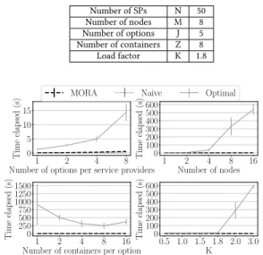
Table 2: Default values of the reference scenario evaluated
Number of SPs N 50 Number of nodes M 8 Number of options J 5 Number of containers Z 8 Load factor K 1.8 1 2 4 8 Number of options per service providers
0 5 10 15 Time elapsed (s)
MORA Naive Optimal
1 2 4 8 16 Number of nodes 0 100 200 300 400 500 600 Time elapsed (s) 1 2 4 8 16 Number of containers per option
0 250 500 750 1000 1250 1500 Time elapsed (s) 0.5 1.0 1.5 1.8 2.0 3.0 K 0 100 200 300 400 500 600 Time elapsed (s)
Figure 3: Time to compute solutions for ILP, MORA and Naive strategies
which results in a diminishing return: the more resources are used by a SP configuration, the larger one should expect the utility to be, but the additional utility tends to decrease with the resources.
Using the notation (6) forwi, j
CP U, w i, j
RAM, the utility is the following
function of the required resources:
ui, j=αi, j⋅ ( w i, j CP U cCP U,tot) 1 βCP Ui, j + (1 − αi, j) ⋅ ( w i, j RAM cRAM,tot) 1 βRAMi, j (12) whereαi, j, βi, j CP U, β i, j
RAMare sampled, for each option, from random
uniform distributions between 0 and 1 forαi, jand between 1 and
5 forβi, j
CP Uandβ i, j
RAM. Since these parameters are random variable,
(12) “loosely” show monotonicity and concavity, but is not exactly a
monotone and concave function. We did this on purpose since: (i) in realistic scenarios this relation may not be as “clean” as assuming a
perfectly increasing and concave function; (ii) we want to check the performance of our solution in pessimistic and ‘unclean” situations. Note that our construction follows the assumptions usually adopted
in the literature [7, 10, 14, 20]. We will not need these assumptions anymore when working with Alibaba traces.
Note that, for all feasible options,ui,z ∈[0, 1]. Since a feasible
solution selects at most one option per SP, we can be sure that
umax
≔N is an upper bound to utot. We define theoverall
normal-ized utility asu = utot/umax (13). By slight abuse of terminology,
in what follows we will shortly refer to “utility” to indicate the overall normalized utility.
6.1.1 Time efficiency. Fig. 3 shows that the computation of the
Optimum from the ILP is too slow for the allocation frequency envisaged in practical deployments, as discussed in §1. On the
contrary, MORA remains within 0.05s, as the Naive policy, while also achieving almost optimal utility, as next sections will show..
1 2 4 8 Number of options per service providers 0 10 20 30 40 50 Utilit y (%)
Optimal MORA Naive
1 2 4 8
Number of options per service providers 0 5 10 15 20 25 30 Av ailable resources (%) CPU (Optimal) RAM (Optimal) CPU (MORA) RAM (MORA) CPU (Naive) RAM (Naive)
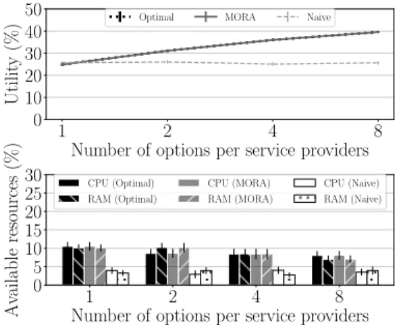
Figure 4: Benefits of multiple options.
6.1.2 Benefits of multiple options. Fig. 4 shows that utility
in-creases with the number of options per SP. Note that the classic
assumption corresponds to the first point of the plot, SP=1. While varying the number of options from 1 to 8 the utility has a gain
almost equal to 60%, which would be lost with classic approaches and which instead we can grasp by exploiting service elasticity.
This is equivalent to virtually increase the available resources, by just using them better. Observe also that MORA uses resources as the optimum, while Naive, despite providing poor utility, uses ~3.3
times more resources than optimal/MORA).
6.1.3 Insensitivity to scaling. We verified that, if we increase the
number of nodes available (thus increasing the overall resources) and we increase accordingly the the option requirements, in order
to always keep a load factorK equal to the default value, the utility
is not affected. We omit the plot for lack of space. This tells us that the results presented here are likely to be consistent even when
scaling the problem and would hold on tiny instances of EC as well as in larger EC clusters.
6.1.4 The more you containerize, the better the utility. Fig. 5,
re-ports for MORA a 11% increase of utility when providing a service through a set of micro-services [26] running on different containers
instead of a single one. Indeed, keeping the same overall resource requirements, “smaller” containers are easier to place into Edge
nodes.
6.1.5 Effects of load (Fig. 6). Increasing the load K (11), we are
increasing the amount of resource contention among SPs. Recall
thatK = 0.5 denotes requests with overall resource requirements
that are half of the available resources. In this case, the highest
utility-option of each SP is likely to be satisfied. ForK ≤ 2, the
more theK, the more utility, from 28% to 40%. This is expected since
(i) increasing theK, we are increasing the resource requirements of
each option and (ii) the utility of each option is randomly generated as an increasing function (12) of the resources. However, if the
load factor increases more than 2 the utility starts to decrease both for the ILP and MORA and equals the naive policy. Further
investigation is required to explain this behavior in our future work.
1 2 4 8 16
Number of containers per option 0 10 20 30 40 50 Utilit y (%)
Optimal MORA Naive
1 2 4 8 16
Number of containers per option 0 5 10 15 20 25 30 Av ailable resources (%) CPU (Optimal) RAM (Optimal) CPU (MORA) RAM (MORA) CPU (Naive) RAM (Naive)
Figure 5: Effect of containerization.
0.5 1.0 1.5 1.8 2.0 3.0 K 0 10 20 30 40 50 Utilit y (%)
Optimal MORA Naive
0.5 1.0 1.5 1.8 2.0 3.0 K 0 20 40 60 80 100 Av ailable resources (%) CPU (Optimal) RAM (Optimal) CPU (MORA) RAM (MORA) CPU (Naive) RAM (Naive)
Figure 6: Effects of load.
Hypothesis are: (i) there is a concave relation between resources
and utilities (see (12)), which reflects in the diminishing returns
observed when increasingK, and the the resources utilized; (ii) as
resources demanded by the containers become larger asK increases,
it is more difficult to place them, which is confirmed by the fact that
the overall resources used withK = 2 and K = 3 remain unchanged.
From these results, at least in our scenarios, we observe that after a certain load threshold the network operator should increase the
Edge resources in order to maintain utility levels. As expected, the bottom figure shows that the NO needs to consume more resources
to satisfy higher loads.
6.1.6 Distribution of resources and utility among SPs . In this
pa-per we mainly consider that utility benefits NO, but in reality it
also benefits SPs. Therefore, it is important to check if resource allocation is fair. Fig. 7 reports the result from one run with 50 SPs.
On the left, the points along each line represent the utility of the
different options declared by one SP. The “◆” is the option chosen
Resource Allocation for Edge Computing with Multiple Tenant Configurations SAC ’20, March 30-April 3, 2020, Brno, Czech Republic 0.1 0.2 0.3 0.4 0.5 0.6 Utility 0 10 20 30 40 50 Service pro vider ID Available option Chosen option 0 50 100 150 200 250 CPUs 0 50 100 150 200 250 RAM (Gb) Chosen option
Figure 7: Distribution of resources and utility between 50 SPs. The x and y scale of the right plot are the total avail-able RAM and CPUs.
thus the others do not get any resources since their contribution to
the overall utility would not be remarkable. In the right plot, the points are the requirements of the options of the 11 SPs chosen to
be deployed in the Edge. From the plot, MORA allocates a similar amount of resources to the selected SPs, which does not necessarily
reflect in equality of utilities selected.
6.2
Results on real traces
We now use Google [2] and Alibaba [1] cluster traces. We assume
8 nodes are available, as in table 2.
Google traces includes a list of jobs, each composed by a set of
tasks. We consider the requested RAM and CP U associated to each task when the correspondent at time of job’s submission. These values are expressed as a fraction of the available resources. To
represent a SPi, we randomly select J jobs and we interpret each as
an optioni, j. Each task composing that job is mapped to a container
z. We used (12) to compute the utility of each option.
Alibaba traces include a list of applications, each comprised of
several containers sharing the same application index. We map an Alibaba application to an option. As in the Google case, We generate
each SP by randomly select a set of options (Alibaba applications). In Alibaba traces, RAM requirements are expressed as percentage of RAM available in one node while CP U requirements are expressed
as percentage of usage of one single core. Each machine in Alibaba cluster has 96 cores. We set the nodes in the simulations to reflect
these requirements.
The trace also reports the bandwidth associated to a container.
We calculate the bandwidth of each option as the sum of the band-width of the containers of the corresponding application. This is
the value of utility that we use. The rational is that we assume that a SP generates a certain traffic toward users. If we select a certain option of a SP, the correspondent bandwidth is served locally at
the edge and only the remaining part part must be served by the Cloud, an assumption common in the literature [13]. Therefore, the
value of the utility indicates the bandwidth saving in this case.
6.2.1 Effects of number of SPs. Fig. 9 and 8 confirm what was
observed in the synthetic scenario. Both in the Google and the
Figure 8: Utility while varying the number of SPs and the number of options provided using Alibaba Traces
Figure 9: Relative utility while varying the number of SPs and the number of options provided using Google Traces
Alibaba case the utility increase when exploiting service elasticity increasing the number of options per SP. We also vary the number of SPs considered, which result in an increase in the load, which we
quantify with ¯KCP Uand ¯KRAM, reported in the figure and calculated
as: ¯ Kl = ¯Wl⋅ N ⋅Z¯/ M ∑ m=1 cl,m
whereW¯l is the average requirement of resource l through all the
containers and ¯Z is the average number of containers per option, l is
{RAM,CPU }. In the Alibaba figure, as expected, the more SPs join the Edge, the more the utility (bandwidth saving) is achievable. In
the Google figure, instead, we report the normalized utility (13) (the
total utility can be obtained by multiplying it byN ). Observe that
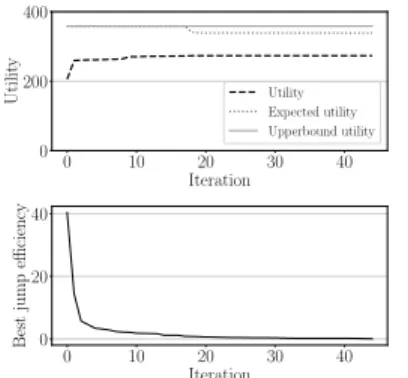
0 10 20 30 40 Iteration 0 200 400 Utilit y Utility Expected utility Upperbound utility 0 10 20 30 40 Iteration 0 20 40 Best jump efficiency
Figure 10: Utility and Best jump efficiency by time
are also the Google, Alibaba and synthetic scenarios. However, the
benefits of service elasticity consistently show themselves.
6.2.2 MORA as anytime algorithm. We use here Alibaba traces,
assuming 8 nodes and 20 SPs. We show in Fig. 10 the utility of
the solution computed at every iterationt. By construction, the
efficiencyEi of the best jump (bottom plot) is decreasing witht.
This ensures that most of the utility is already achieved in the first iterations (top plot) and allows us to prematurely stop the algorithm
if the time available to compute the allocation is scarce, still having a good solution at hands. The upper bound to the optimal solution
(§5.3.2) reported in the figure also confirms that we are already close to the optimum in the first iterations. By exploiting the fact
the monotonicity ofEiwe can also easily calculate, at any iteration
t, the Expected utility, i.e., the utility that we can achieve at most if we continue the algorithm until the end instead of interrupting at t. We omit the details of this calculation for lack of space, but we report it in the figure to show that it can also be a useful guidance
to decide whether to stop MORA before its end for a faster result.
7
CONCLUSIONS AND FUTURE WORK
This paper presented MORA, a strategy for resource allocation for Edge Computing (EC), where tenants are third party Service Providers (SPs). The novelty of this work is that it exploits service
elasticity: by allowing SPs to declare the different configurations (aka options) in which they can run, we show that the Network
Operator (NO) owning EC resources can greatly increase utility. Relying on service elasticity is crucial in resource-constrained
en-vironments as EC.
Our future work will be devoted to scenarios where SPs arrive
at different times, exploiting a time-batched implementation of the heuristic. We plan to realize a testbed using Docker and Kubernetes. Moreover, the architecture and the heuristic itself have to be
ex-panded in order to take into account different NOs (Edge roaming). We consider using Game Theory to design mechanisms to ensure
truthful declaration of options by SPs, which could also be enforced by appropriate resource and utility monitoring. We are also
inter-ested in studying allocation strategies in presence of noise in the values of resource usage and utility.
REFERENCES
[1] [n. d.]. Alibaba Cluster Trace Program.([n. d.]). https://github.com/alibaba/ clusterdata
[2] [n. d.]. Google Borg Cluster usage traces. ([n. d.]). https://github.com/google/ cluster- data
[3] [n. d.]. OpenConnect service by Netflix. ([n. d.]). https://openconnect.netflix. com/en/
[4] A. Di Stefano A. Di Stefano and G. Morana. 2020. Scheduling communication-intensive applications on Mesos.IJGUC 11, 1 (2020), 103–114. https://doi.org/10. 1504/IJGUC.2020.103974
[5] Y. Al-Dhuraibi et al. 2017. Autonomic Vertical Elasticity of Docker Containers with ELASTICDOCKER. InIEEE CLOUD.
[6] Andrea Araldo, Alessandro Di Stefano, and Antonella Di Stefano. 2020. Edge-MORE: Improving Resource Allocation with Multiple Options from Tenants. In IEEE Consumer Communications & Networking Conference (CCNC). Las Vegas, USA.In-Press.
[7] A. Araldo, G. DÃąn, and D. Rossi. 2018. Caching Encrypted Content Via Stochastic Cache Partitioning.IEEE/ACM Transactions on Networking 26, 1 (Feb 2018), 548– 561.https://doi.org/10.1109/TNET.2018.2793892
[8] Sergei Arnautov et al. 2016. SCONE: Secure Linux Containers with Intel SGX. In USENIX Symp. on Op. Sys. Des. and Impl. 689–703.
[9] Francesco Bronzino et al. 2019. Lightweight , General Inference of Streaming Video Quality from Encrypted Traffic. (2019). arXiv:arXiv:1901.05800v2 [10] Weibo Chu et al. 2018. Joint cache resource allocation and request routing for
in-network caching services.Comp. Net. 131 (2018), 1–14. arXiv:arXiv:1710.11376v2 [11] A. Di Stefano, A. Di Stefano, G. Morana, and D. Zito. 2018. Coope4M: A Deploy-ment Framework for Communication-Intensive Applications on Mesos. In2018 IEEE 27th International Conference on Enabling Technologies: Infrastructure for Collaborative Enterprises (WETICE). 36–41. https://doi.org/10.1109/WETICE.2018. 00014
[12] Koustabh Dolui and Soumya Kanti Datta. 2017. Comparison of edge computing implementations: Fog computing, cloudlet and mobile edge computing.2017 Global Internet of Things Summit (GIoTS) (2017), 1–6.
[13] M. Enguehard, G. Carofiglio, and D. Rossi. 2018. A Popularity-Based Approach for Effective Cloud Offload in Fog Deployments. InITC.
[14] S. Ghosh et al. 2003. Scalable resource allocation for multi-processor QoS opti-mization. InIEEE ICDCS. 174–183.
[15] Yichao Jin, Yonggang Wen, and Cedric Westphal. 2015.Optimal Transcoding and Caching for Adaptive Streaming in Media Cloud.IEEE Trans. Circ. and Sys. Video Tech. 25, 12 (2015), 1914–1925.
[16] Sladana Josilo et al. 2019. Wireless and Computing Resource Allocation for SelfishComputation Offloading in Edge Computing. InIEEE INFOCOM. [17] Sladana Josilo and Gyorgy Dan. 2018.Selfish Decentralized Computation
Of-floading for Mobile Cloud Computing in Dense Wireless Networks.IEEE Trans. Mobile Comput. 1233, c (2018).
[18] Hans Kellerer, Ulrich Pferschy, and David Pisinger. 2004.Knapsack Problems (1st ed.). Springer.
[19] David G Kirkpatrick and Raimund Seidel. 1986. The ultimate planar convex hull algorithm?SIAM J. on Comp. 15, 1 (1986), 287–299.
[20] C. Lee, J. Lehoczky, D. Siewiorek, R. Rajkumar, and J. Hansen. 1999. A scalable solution to the multi-resource QoS problem. InIEEE Real Time Systems Symp. [21] J. Liang et al. 2014. When HT TPS Meets CDN: A Case of Authentication in
Delegated Service. InIEEE Symp. on Security and Privacy.
[22] Bruce M. Maggs and Ramesh K. Sitaraman. 2015. Algorithmic Nuggets in Content Delivery.ACM SIGCOMM CCR 45, 3 (2015), 52–66.
[23] S. Maheshwari et al. 2018. Scalability and Performance Evaluation of Edge Cloud Systems for Latency Constrained Applications. In2018 IEEE/ACM Symp. on Edge Computing (SEC). 286–299.
[24] Hongzi Mao et al. 2016. Resource Management with Deep Reinforcement Learn-ing. InACM Hotnet Workshop.
[25] J. Monsalve, A. Landwehr, and M. Taufer. 2015. Dynamic CP U Resource Allo-cation in Containerized Cloud Environments. In2015 IEEE Int. Conf. on Cluster Computing. 535–536.
[26] C. Pahl and B. Lee. 2015. Containers and Clusters for Edge Cloud Architectures -a Technology Review. InIEEE FiCloud2.
[27] B. P. Rimal et al. 2018. Experimental Testbed for Edge Computing in Fiber-Wireless Broadband Access Networks.IEEE Com.Mag. 56, 8 (2018), 160–167. [28] Y. Song et al. 2008. Multiple multidimensional knapsack problem and its
applica-tions in cognitive radio networks. InIEEE Military Comm. Conf.
[29] Y. Tao et al. 2017. Dynamic Resource Allocation Algorithm for Container-Based Service Computing. InIEEE ISADS.
[30] Liang Tong, Yong Li, and Wei Gao. 2016. A hierarchical edge cloud architecture for mobile computing. InIEEE INFOCOM.
[31] Doron Zarchy et al. 2015. Capturing resource tradeoffs in fair multi-resource allocation. InIEEE INFOCOM.
[32] D. Zhang and pthers. 2017. Container oriented job scheduling using linear programming model. InICIM.