HAL Id: lirmm-00385149
https://hal-lirmm.ccsd.cnrs.fr/lirmm-00385149
Submitted on 18 May 2009HAL is a multi-disciplinary open access archive for the deposit and dissemination of sci-entific research documents, whether they are pub-lished or not. The documents may come from
L’archive ouverte pluridisciplinaire HAL, est destinée au dépôt et à la diffusion de documents scientifiques de niveau recherche, publiés ou non, émanant des établissements d’enseignement et de
Imprecise Expectations for Imprecise Linear Filtering
Agnès Rico
To cite this version:
Agnès Rico. Imprecise Expectations for Imprecise Linear Filtering. [Research Report] RR-09011, LIRIS. 2009, pp.1-26. �lirmm-00385149�
Imprecise expectations for imprecise linear
filtering
A. Rico
a,∗, O. Strauss
baLIRIS Universit´e Claude Bernard Lyon 1, 43 bld du 11 novembre 1918, 69622
Villeurbanne, France
bLIRMM Universit´e Montpellier II, 61 rue Ada, 34392 Montpellier cedex 5,
France
Abstract
In the last 10 years, there has been increasing interest in interval valued data in signal processing. According to the conventional view, an interval value suppos-edly reflects the variability of the observation process. Generally, the considered variability is associated with either random noise or the uncertainty that underlies the observation process. In most sensor measure based applications, the raw sensor signal has to be processed by an appropriate filter to increase the signal to noise ratio or simply to recover the signal to be measured. In both cases, the output filter is obtained by convoluting the sensor signal with a supposedly known appropriate impulse response. However, in many real life situations, this impulse response can-not be precisely specified. The filtered value can thus be considered as biased by this arbitrary choice of one impulse response among all possible impulse responses considered in this specific context. In this paper, we propose a new approach to perform filtering that aims at computing an interval-valued signal that contains all outputs of filtering processes involving a coherent family of conventional linear fil-ters. This approach is based on a very straightforward extension of the expectation operator involving appropriate concave capacities.
Key words: Linear filtering, expectation, interval valued signal, Choquet integral, non-additive confidence measure.
∗ Corresponding author.
Email addresses: [email protected](A. Rico ), [email protected] (O. Strauss ).
1 Introduction
In the last 10 years, there has been increasing interest in interval valued data [11]. Generally, replacing a precise value by an interval value generally reflects the variability or uncertainty that underlies the observation process. There are, however, different possible interpretations of an interval in the framework of data analysis and processing. An interval value can be seen as:
• a range in which one could have a certain level of confidence of finding the true value of the observed variable [24],
• a range of values that the real data can take when the measurement process involves quantization and/or sampling [11,12],
• representation of the known detection limits, sensitivity or resolution of a sensor [15].
In signal processing, a major difficulty is often to have access to a process with a truly reliable knowledge on the properties of the expected variations and errors that contaminate the observations. In the state estimation context, some very well established state estimation processes, e.g. Kalman filtering, can lead to developments that are mathematically complicated and exceed the engineer’s expertise in process control. To overcome this difficulty, some interval observation based algorithms have been proposed for state estimation (see e.g. [22,4]). The same problem arises in the sensor fusion setting. In [24], an interval estimation fusion based on sensor interval estimates is considered that leads to fused values that have advantages with respect to their precise equivalents in terms of robustness, specificity and easy extension to higher dimensionality. In [9], Brito considered replacing precise valued by interval valued data to perform a robust data analysis.
However, within any interval-based signal processing application, there is still a strong need for a reliable representation of the variability domain of each involved observation. An important issue concerns the meaning of the inter-val and the consistency of this meaning with respect to the tools used for a further analysis or processing. In many practical applications, a confidence in-terval with a probability of one is too wide to obtain useful values. Therefore, one problem of practical interest is to be able to obtain an interval valued ob-servation with a particular guaranteed property but which is also as specific as possible.
Single or double bootstrapping has been proposed as a nice way for recovering the confidence interval of an estimated value [17]. However, the computing resources required by such methods may be prohibitive. In [13], a Monte-Carlo method based on a Cauchy distribution is used to provide the interval valued expected error of a function whose inputs are intervals. Quantile estimates can
also be involved to obtain specific confidence intervals [3].
Random set theory would be required to use these interval data (see e.g. [9] and references therein). Kreinovich et al. [15] propose to extend expectation or variance of interval valued data. In [8], the authors propose to design an interval observer of a time varying process that provides online estimation of upper and lower bounds of unmeasured states of the observations. This estimation is said to contain, with certainty, the true observation based on supposed pre-knowledge of the input signal bounds and reasonable knowledge on the equation that applies to the observed process. An interesting property is that generally the width of the observed interval directly depends on the uncertainty range of the unknown variables.
This property can be very useful for signal processing applications. Moreover, it would be necessary to account for a known pre-calibrated observation vari-ability, but also for a lack of knowledge on the proper model to be used. In this context, here we propose a new interpretation of an interval-valued piece of information.
Consider a linear process involving an expectation-like operation for which you have partial information about the suitable probability function to be used. Thus, a way to account for this mis-knowledge is to consider every possible (suitable) function. Then the exact output value of the process cannot be pre-cisely computed. It seems natural to replace the notion of precise expected value by an imprecise expected value that represents all possible precise ex-pected values given by all possibly appropriate models. An interval can be a compact and useful representation of this imprecise expected value.
The problem of computing an expected value based on an ill-known proba-bility has been proposed in the past in the decision making context (see [23] and references therein). The more general framework involves sets of probabil-ities called credal sets [18]. However, expectation based on general credal sets often lead to computationally complicated methods involving at least linear constrained programming. A simpler way to account for the mis-knowledge on the suitable probability to be used is to consider an interval-based repre-sentation of the cumulative distribution function (cdf). This approach, also called p-box [1], has been successfully used in the past (see references in [13]). However, as shown by Kreinovich and Ferson in [14], this representation can sometimes lead to estimates that are not specific enough, in contradiction with the underlying confidence representation, or else to NP-hard computa-tions. Interval-valued probabilities have also been studied [23] but, considering reasonable requirements, this approach leads to a precise valued expectation operator. A more specific and very useful way of representing probability den-sity function (pdf) family is to consider a class of non-additive confidence measures called concave Choquet capacities [2].
In this paper, we propose to represent the notion of partial lack of probabilistic information by replacing the pdf, commonly used for performing aggregation in signal processing applications, by a concave capacity. Such a capacity aims at representing a convex hull of a credal set called the core of this capacity. We thus propose a very simple extension of the expectation operator whose output is an interval instead of a single value. We show that this interval is the most specific that includes every precise expected value based on a probability that belongs to the core of the capacity. This generalization makes use of asymmetric or symmetric Choquet integrals. Then, by considering the conventional linear filtering as a linear combination of at most two linear expectations, we make use of our new interval valued expectation operator to design interval valued output filtering processes that contains all the outputs of filtering processes involving a coherent family of conventional linear filters. This article is organized as follows: section 2 presents the framework and notations. Section 3 deals with the construction of our imprecise expectation operators. Section 4 explains how to use our imprecise operators for performing imprecise filtering. Section 5 presents some illustrative experiments.
2 Framework and notations
In this section, we present notations, definitions and technical results useful for this article. A first part introduces the notations. A second subsection briefly presents the expectation operator. A third part deals with symmetric and asymmetric Choquet integrals. Finally, a last subsection recalls some results concerning generalized real intervals.
2.1 Notations
This section presents the notations which will be used througout this article. • Ω = {1, . . . , N} is a finite set,
• P(Ω) is the set of subsets of Ω,
• X : Ω → IR denotes a real function defining the observation process on Ω, • V = {X : Ω → IR} is the set of all real functions on Ω,
• ∀n ∈ {1, . . . , N}, ∀X ∈ V , X(n) is denoted Xn and throughout this paper
we denote X = (Xn)n=1,...,N.
• ρ : Ω → [0, 1] is the probability associated to each observed value. ∀n ∈ {1, . . . , N}, ρ(n), denoted ρn, is the probability associated to the nth
ob-servation.
2.2 The expectation operator
In probability theory, the expected value of a discrete random variable is the sum of probabilities of each possible outcome of the experiment multiplied by the outcome value. It represents the average when identical odds are repeated many times.
Considering N observations, {X1, . . . , XN}, the expected value of X based on
the probability distribution ρ is: Y =
N X n=1
ρnXn
Note that the aggregated value Y considering the N observations is obtained by a weighted sum. A minimal requirement for such an operator is:
minn∈{1,...,N }Xn ≤ Y ≤ maxn∈{1,...,N }Xn.
Moreover, if all observations equal a same real value c, then the expected value should equal to c. This property leads to
N X n=1
ρn = 1. More precisely, ρ is a
discrete probability measure P on each subset of Ω:
∀A ⊆ Ω, P (A) = X
n∈A
ρn.
Based on this probability measure P , one can define the expectation operator as follows:
Definition 1 Let X ∈ V be a real function on Ω and ρ be a probability asso-ciated to each values which defines a probability measure P . The expectation of X according to P is defined by:
Y = EP(X) = X n∈Ω
ρnXn. (1)
A first straightforward idea to account for ill known probability weights is to replace the precise probability in expression (1) by an interval valued probabil-ity [ρn, ρn]. However, as shown in [23], when this aggregation to be consistent
with the usual precise probability based aggregation, this approach leads to a very simple but precise expected value, which does not comply with the desired properties.
2.3 Symmetric and asymmetric Choquet integral
This section presents the symmetric and the asymmetric Choquet integral with some useful properties.
Definition 2 • A capacity v is a set function v : P(Ω) → [0, 1] such that v(∅) = 0, v(Ω) = 1, and ∀A ⊆ B ⇒ v(A) ≤ v(B).
• vc, the conjuguate1capacity of v, is the capacity defined by:
∀A ∈ P(Ω), vc
(A) = 1 − v(Ac),
where Ac denotes the complementary set of A in Ω.
• A capacity v is concave if and only if
∀A, B ∈ P(Ω), v(A ∪ B) + v(A ∩ B) ≤ v(A) + v(B). • The core of a capacity v is
core(v) = {P probalility on P(Ω) such that v(A) ≤ P (A), ∀A ∈ P(Ω)}.
Let X ∈ V be a function, then (·) denotes the permutation function on the set {1, . . . , N} such that the function X is a non-decreasing function. More precisely, we have X(1) ≤ . . . ≤ X(N ). Hence, ∀i ∈ {1, . . . , N}, A(i) is the set
defined by A(i) = {(i), . . . , (N)}. When the values of a function X are positive,
we can define the Choquet integral of X.
Definition 3 Let X : Ω → IR+ be a function and v be a capacity on P(Ω). • The Choquet integral of X with respect to the capacity v is:
Cv(X) = N X n=1
X(n)(v(A(n)) − v(A(n+1))) with A(N +1) = ∅
• A dual Choquet integral can be computed using the conjuguate capacity: Cvc(X) = N X n=1 X(n)(v(Ac(n+1)) − v(A c (n))).
When X is a real function two solutions exist to extend the Choquet integral: the asymmetric Choquet integral and the symmetric Choquet integral, also called the ˇSipoˇs integral.
1 The classical ¯
vnotation will not be used in this paper so as to make the equations below more easily understandable.
Definition 4 Let X ∈ V be a function, we define the positive functions X−
and X+ as follows:
∀n ∈ {1, · · · , N}, X−
n = max(−Xn,0) and Xn+= max(Xn,0).
Throughout this article, we refer to X− = max(−X, 0) and X+= max(X, 0),
where 0 denotes the function equal to 0 everywhere.
The asymmetric Choquet integral and the symmetric Choquet integral are defined as follows:
Definition 5 Let X be a function from Ω = {1, . . . , N} to IR.
• The asymmetric Choquet integral of function X with respect to a capacity v is:
ˇ
Cv(X) = Cv(X+) − Cvc(X−).
• The symmetric Choquet (or ˇSipoˇs ) integral of function X with respect to a capacity v is:
ˇ
Sv(X) = Cv(X+) − Cv(X−).
Both asymmetric and symmetric Choquet integrals are non-decreasing func-tions, but they do not have the same behavior, for example we have the fol-lowing property:
Proposition 6 Let X ∈ V be a real function on Ω.
∀α > 0, ∀β ∈ IR, ˇCv(αX + β) = ˇCv(αX1+ β, . . . , αXN + β) = α ˇCv(X) + β,
∀α ∈ IR, ˇSv(αX) = α ˇSv(X),
Proof:See [7].
2.4 Generalized real intervals
Using the symmetric Choquet integral to generalise the expectation operator can lead to an improper interval valued output.
A generalized real interval a is denoted a = [α, β] with α, β ∈ IR such that the inequality α ≤ β is not always satisfied [11]. There are two sorts of intervals: proper intervals and improper intervals:
• A proper interval is an interval [α, β], α, β ∈ IR where α ≤ β. • An improper interval is an interval [α, β], α, β ∈ IR where β ≤ α.
In this article, we use the following generalized interval operators. Let a = [α, β] be a generalized interval.
dual(a) = [β, α], pro(a) = a if a is a proper interval dual(a) else.
Definition 7 When a = [α, β], α, β ∈ IR is a generalized interval, then [a] = pro(a) = [a, a] denotes the proper interval such that a = min(α, β) and a= max(α, β).
IIIR denotes the set of proper intervals of IR.
Definition 8 Let [a], [b] ∈ IIIR be two proper intervals, • the Minkowski addition is: [a] ⊕ [b] = [a + b, a + b], • the dual Minkowski addition is: [a] ⊞ [b] = [a + b, a + b].
As [a] and [b] are two proper intervals, [a] ⊕ [b] is a proper interval but [a] ⊞ [b] is not always a proper interval.
If 0 ∈ [b], then the Minkowski addition can be interpreted as a dilation, and the dual Minkowski addition can be interpreted as an erosion [19].
Note that [a] ⊞ [b] = [a] ⊕ dual([b]).
We also defined two substraction operators:
Definition 9 Let [a], [b] ∈ IIIR be two poper intervals. • [a] ⊖ [b] = [a, a] ⊕ [−b, −b] = [a − b, a − b],
• [a] ⊟ [b] = [a, a] ⊞ [−b, −b] = [a − b, a − b].
⊖ is the Minkowski subtraction and the ⊟ operator is identical to the difference operator defined by Hukahara in [10] when [a] = [b]⊕[x] has a proper solution.
3 Imprecise expectation operators, Ev(·) and ∃v(·), according to a
concave capacity v.
This section deals with the presentation of Ev(·) and ∃v(·) which are operators
Let Ω be a finite set of N elements, v be a concave capacity on P(Ω) and vc be the conjuguate capacity of v. The functions on Ω are denoted X and
the set of all functions is denoted V . When X ∈ V , we use the decomposition X = X+−X−presented in Definition 4. To begin, let us recall a result proved
by Denneberg [5]:
Theorem 10 If v is a concave capacity on P(Ω), then • ∀X ∈ V, ˇCv(X) = sup P∈core(vc) EP(X), • ∀X ∈ V, ˇCvc(X) = inf P∈core(vc)EP(X), • ∀X ∈ V, ˇCvc(X) ≤ ˇCv(X),
where EP(·) is the expectation operator according to probability P .
So we can define a minimum operator and a maximum operator, denoted respectively ˇCvc : V → IR and ˇC
v : V → IR. Hence, a proper interval
[ ˇCvc(X), ˇCv(X)] can be associated with each function X ∈ V . Note that, if v is a concave capacity and if ∀P ∈ core(vc), E
P(X) are equal and
then ˇCvc(X) = ˇCv(X). If X is a constant function equal to c, then ˇCvc(X) = ˇ
Cv(X) = c.
When working with the symmetric Choquet integral, the order relation be-tween ˇSvc(X) and ˇSv(X) is unknown, so the interval [ ˇSvc(X), ˇSv(X)] can be an improper inteval. In such cases, we have to specify pro([ ˇSvc(X), ˇSv(X)]), where pro(·) is the operator defined in subsection 2.4. Hence, we have the following definition:
Definition 11
Ev : V → IIIR and ∃v : V → IIIR
X 7→ [ ˇCvc(X), ˇC
v(X)] X 7→ pro([ ˇSvc(X), ˇS
v(X)]).
Note that if X ∈ V is a positive function, then the asymmetric Choquet integral and the symmetric Choquet integral are equal and coincide with the Choquet integral. In this case, Ev(·) denotes this common operator.
Ev(·) and ∃v(·) are two imprecise expectation operators based on the concave
confidence measure v. We now present some useful properties of these new operators.
Proposition 12
Proof:v is a concave capacity so, according to Theorem 10,
∀X ∈ V, Cvc(X) ≤ Cv(X). Using the definition of symmetric and asymmetric Choquet integrals, the following equalities can be written:
• ˇSv(X) = Cv(X+) − Cv(X−) ≤ Cv(X+) − Cvc(X−) = ˇCv(X). • ˇSvc(X) = Cvc(X+) − Cvc(X−) ≤ Cv(X+) − Cv(X−) = ˇCv(X). • ˇSvc(X) = Cvc(X+) − Cvc(X−) ≥ Cvc(X+) − Cv(X−) = ˇCvc(X). • ˇCvc(X) − ˇSv(X) = Cvc(X+) − Cv(X−) − Cv(X+) + Cv(X−) =
Cvc(X+) − Cv(X+) ≤ 0.
So we have proved that ˇCvc(X) ≤ min( ˇSv(X), ˇSvc(X)) and max( ˇSv(X), ˇSvc(X)) ≤ ˇ
Cv(X).
Definition 13 ∀X ∈ V , Sv(X) = min( ˇSvc(X), ˇSv(X)) and Sv(X) = max( ˇSvc(X), ˇSv(X))
denote the bounds of ∃v(X).
Proposition 14 ∀X ∈ V, the inclusion ∃v(X) ⊆ Ev(X) is symmetric, i.e the
equality ˇCv(X) − Sv(X) = Sv(X) − ˇCvc(X) is satisfied ( see Figure 1 ).
Proof:We have to prove that ˇCv(X) − Sv(X) = Sv(X) − ˇCvc(X). ˇ Cvc(X) Sv(X) Sv(X) ˇ Cv(X) (Cv− Cvc)(X−) (C v− Cvc)(X+) (Cv − Cvc)(X+) (Cv− Cvc)(X−)
Fig. 1. ”Symmetric” inclusion
ˇ Cv(X) = Cv(X+) − Cvc(X−) = Cv(X+) − Cv(X−) + Cv(X−) − Cvc(X−) = ˇSv(X) + (Cv− Cvc)(X−) ˇ Cvc(X) = Cvc(X+) − Cv(X−) = Cvc(X+) − Cvc(X−) + Cvc(X−) − Cv(X−) = ˇSvc(X) − (Cv− Cvc)(X−) So we have ˇCv(X) − ˇSv(X) = ˇSvc(X) − ˇCvc(X). ˇ Cv(X) = Cv(X+) − Cvc(X−) = Cv(X+) − Cvc(X+) + Cvc(X+) − Cvc(X−) = ˇSvc(X) + (Cv− Cvc)(X+) ˇ Cvc(X) = Cvc(X+) − Cv(X−) = Cv(X+) − Cv(X+) + Cvc(X+) − Cv(X−) = ˇSv(X) − (Cv − Cvc)(X+)
So we have ˇCv(X) − ˇSvc(X) = ˇSv(X) − ˇCvc(X).
Corollary 15 Let X ∈ V such that X = X+− X−. Hence,
(Cv − Cvc)(X−) < (Cv− Cvc)(X+) ⇔ S v(X) = Svc(X) and ¯S(X) = Sv(X) (Cv − Cvc)(X−) = (Cv− Cvc)(X+) ⇔ S v(X) = Svc(X) = ¯S(X) = Sv(X) Proof: Svc(X) − Sv(X) = Cvc(X+) − Cvc(X−) − (Cv(X+) − Cv(X−)) = (Cvc − Cv)(X+) − (Cvc− Cv)(X−).
Note that if X ∈ V is a real function such that X+ = X−, then S
vc(X) = Sv(X). This property is not satisfied for Cvc(X) and Cv(X).
Proposition 16
∀X ∈ V, Ev(X) = Ev(X+) ⊖ Ev(X−)
∀X ∈ V, ∃v(X) = pro(Ev(X+) ⊟ Ev(X−))
Proof:We have Ev(X+) = [ ˇCvc(X+), ˇCv(X+)] and Ev(X−) = [ ˇCvc(X−), ˇCv(X−)]. Hence using Definition 9,
Ev(X+) ⊖ Ev(X−) = [ ˇCvc(X+) − ˇCv(X−), ˇCv(X+) − ˇCvc(X−)] = [ ˇCvc(X), ˇCv(X)]
Ev(X+) ⊟ Ev(X−) = [ ˇCvc(X+) − ˇCvc(X−), ˇCv(X+) − ˇCv(X−)] = [ ˇSvc(X), ˇSv(X)].
4 Imprecise expectation for imprecise filtering
Linear filtering consists of convolving an input signal with a particular func-tion called the impulse response of the filter. Since the specific knowledge of the impulse response of the filter cannot usually be justified, it would be use-ful to be able to account for this ill-knowledge by replacing a unique impulse
response by a coherent family of impulse responses. In this section, we propose to use the new operator presented in the previous section to provide such new filtering tools for representing the lack of knowledge on the proper impulse response to be used on the precision of the filter output. We first show that any discrete filter can be considered as a weighted sum of at most two usual expectations. We use this property to design linear filtering processes with an imprecise output. Then we propose a method for designing concave capaci-ties that induce a particular property on the imprecision of the output. This method consist of deriving capacities from the knowledge a user has about the impulse response of one (or more) filters that should be appropriate for the considered application. We propose two approaches to derive an impre-cise filter from a preimpre-cise filter. The first approach consists of constructing the most specific possibilistic capacity that encloses the probabilities involved in the filtering. The second approach simply consists of designing capacities that account for imprecision induced by the sampling.
4.1 Summative kernel based filtering and expectation operators
We consider a discrete summative kernel [16] the impulse response of a discrete filter having only positive values and a unitary gain, i.e. (ρi)i∈ZZ is a discrete
summative kernel if and only if: ∀i ∈ ZZ, ρi ≥ 0 and X
i∈ZZ
ρi = 1.
Since most kernels used in signal processing are bounded, we only consider this case: (ρi)i∈ZZ is bounded, means that ∃N ∈ IN, i 6∈ [−N, N] ⇒ ϕi = 0.
As noted in section 2, a summative kernel defines a probability measure P on
each measurable subset A of ZZ by P (A) = X
i∈A
ρi. Therefore, computing the
discrete convolution of an input signal X = (Xn)n=1,...,N ∈ V is equivalent
to a discrete expectation operation involving the probability measure P . The computation of Yk, the kth component of the filter output is given by:
Yk = N X n=1
ρk−nXn = EPk(X), (2)
with Pk being the probability measure defined by the translated summative
kernel (ρk−n)n∈ZZ.
Proposition 17 Any real finite impulse response of a bounded discrete filter can be expressed as a linear combination of, at most, two summative kernels. Proof:Let (ϕi)i∈ZZ be the real finite impulse response of a discrete filter (i.e.
X
i∈ZZ
ϕi <∞). Let ϕ+i = max(0, ϕi) and ϕ−i = max(0, −ϕi). Let A+ = X i∈ZZ ϕ+i and A− = X i∈ZZ ϕ−i . By construction ϕi = ϕ+i − ϕ−i .Let ρ+i = ϕ+i A+ and ρ − i = ϕ− i A−.
By construction, ρ+i and ρ−i are summative kernels. Now ϕ+i = ρ+i A+ and
ϕ−i = ρ−i A−, therefore ϕi = ρ+i A+− ρ−i A−.
Corollary 18 Any discrete linear filtering operation can be considered as a weighted sum of, at most, two expectation operations.
Corollary 19 Let Pk+ (rsp.Pk− ) be the probability measure based on the
sum-mative kernel ρ+k−i (rsp.ρ−k−i ), then Yk= A+EPk+(X) − A
−E
P−
k (X).
Proof: Let X = (Xn)n=1...N be the discrete signal to be filtered and (ϕi)i∈ZZ
the impulse response or the filter Yk, the kth component of the filter output, is
computed by the discrete convolution of the impulse response of the filter and the imput signal: Yk =
N X n=1 ϕk−nXn. Since ϕi = ϕ+i − ϕ−i , Yk = N X n=1 (ϕ+k−n− ϕ−k−n)Xn = N X n=1 ϕ+k−nXn − N X n=1 ϕ−k−nXn. Now ϕ+i = ρi+A+ and ϕ−i = ρ−i A−, therefore Yk = A+ N X n=1 ρ+k−nXn− A− N X n=1 ρ−k−nXn. By construction, X i∈ZZ ρ+i = 1 and X i∈ZZ ρ−i = 1 ,thus Yk= A+EP+ k(X) − A −E P− k (X). We call the decomposition of (ϕi)i∈ZZ into (ρ+i )i∈ZZ , (ρ
−
i )i∈ZZ, A
+ and A−the
canonical decomposition of ϕ, the impluse response of the filter.
4.2 How can an imprecise filtering operator be derived from a conventional filtering operator ?
Since no tool is currently available to derive a suitable capacity from objective criteria, we propose in a signal processing context, to derive an imprecise filtering operator from one (or several) conventional filters that have been validated for his particular application.
Let us consider a discrete filter whose finite impulse response is (ϕi)i∈ZZ. Let
, us also consider the canonical decomposition of ϕ into ρ+, ρ−, A+ and A−.
Let P+ (rsp. P−) be the probability measure induced by ρ+ (rsp. ρ−). The
method we propose consists of finding two capacities v+ and v− such that
P+ ∈ core(v+) and P− ∈ core(v−). By translating the confidence measures,
Let X = (Xn)n=1...N be the discrete signal to be filtered. Due to the
proper-ties of the imprecise expectation operators, we have EP+(X) ∈ E +
v(X) and
EP−(X) ∈ E −
v(X). Therefore, let Yk be the kth component of the output of
the precise filter:
Yk = A+EPk+(X) − A −E P− k (X) ∈ [Yk] = A +E v+k(X) ⊖ A −E v− k(X) (3) with [Yk] the kth component of the output of the imprecise filter.
Note that in expression (3) the imprecise expectation operator E(·) can also be replaced by the symmetric Choquet integral-based operator ∃(·). Also the Minkowsky subtraction ⊖ can be replaced by the dual Minkowsky subtraction ⊟. Replacing the expectation operator can be warranted if the zero value has a special meaning in the signal. Replacement of the Minkowsky operator can be required if their is a strong link between the two dominated summative kernels ρ+ and ρ− as will be shown in the section 5.2.
4.3 Imprecise filtering based on a possiblity distribution
A possibility measure is a particular concave capacity. In fact, a possibility measure is the only capacity measure (except for the probability measure) that can be defined by a distribution. (πi)i∈ZZ is a possibility distribution if
and only if: πi ≥ 0, ∀i ∈ ZZ and max
i∈ZZ
{πi} = 1.
A possibility distribution induces, on each finite subset A of ZZ, a possibility measure denoted Π(A) that is computed as follows: Π(A) = max
i∈A{πi} = 1.
As shown in [16], the most suitable way to associate a discrete possibility distribution with a discrete probability distribution (ρi)i∈ZZ, in an objective
context, consists of computing the most specific transformation proposed by Dubois and Prade [6]. This transformation leads to defining a possibility dis-tribution (πi)i∈ZZ:
πi = X
k∈ZZ
ρkχ(ρk ≤ ρi), (4)
with χ(ρk ≤ ρi) = 1 if ρk ≤ ρi and 0 otherwise. The possibility measure Π,
induced by (πi)i∈ZZ, is then the most specific that dominates the
probabil-ity measure P induced by (ρi)i∈ZZ. This possibility distribution can also be
thought of as a maxitive kernel [16].
subjec-tive context, called the subjecsubjec-tive transformation and leading to a possibility distribution ( ˜πi)i∈ZZ, such that: ˜πi =
X
k∈ZZ
min(ρk, ρi).
This subjective transformation always defines a possibility distribution that is less specific than the previous one, i.e. ∀i ∈ ZZ, ˜πi ≥ πi.
Finally, since a broad range of summative kernels used for signal processing are monomodal and symmetric, a triangular maxitive kernel is a good candidate since it defines a possibility measure that dominates any probability measure defined by a summative kernel having the same mode and any lower bandwidth [16].
4.4 Imprecise filtering based on accounting for sampling
Another way to derive an imprecise filtering operator from a precise filtering operator is to account for imprecision due to sampling. Indeed, most discrete filters used in digital signal processing are designed to be a sampled version of a continuous filter. Let (ρi)i∈ZZ be the discrete probability distribution
as-sociated with the considered filter. Let us suppose that this distribution is bounded, i.e. there is a subset Ω of ZZ such that ∀i 6∈ Ω, ρi = 0.
The fact that this discrete filter is derived from a continous filter means that each value ρi associated with the ith sampled time (iT ) with T being sample
time, is obtained by integrating a continuous function ρ(t) in a neighborhood of iT defined by a continuous sampling kernel η:
ρi = ∞ Z
−∞
ρtη(t − iT )dt. (5)
The neighborhood sampling kernel (e.g. splines [21]) is usually a monomodal positive function bounded by the interval [−T, T ], such that
∞ Z
−∞
η(t)dt = 1. A way to recover the continuous original function ρ(t) from the discrete kernel (ρi)i∈ZZ, is to use an interpolating kernel. Most of these kernels lead to
Thus a simple way to account for this imprecision is to define a capacity v by: v : Ω → [0, 1] A → v(A) = X k∈Ω φA(k) X k∈Ω φΩ(k) with φA(k) = max(ρk, ρk+1) if k ∈ A and (k + 1) ∈ A ρk if k ∈ A and (k + 1) 6∈ A ρk+1 k 6∈ A and (k + 1) ∈ A 0 else.
Proposition 20 The above capacity is concave.
Proof:Let A, B ∈ Ω, v is concave if v(A)+v(B)−v(A∪B)−v(A∩B) ≥ 0. Let
α= X
k∈Ω
φΩ(k), thus v is concave if αv(A)+αv(B)−αv(A∪B)−αv(A∩B) ≥ 0
i.e X
k∈Ω
(φA(k) + φB(k) − φA∪B(k) − φA∩B(k)) ≥ 0 because α ≥ 0.
To prove the inequality, we consider all possible situations in the following table:
k ∈ A k + 1 ∈ A k ∈ B k + 1 ∈ B φA(k) + φB(k) − φA∪B(k) − φA∩B(k)
yes yes yes yes 0
yes yes yes no 0
yes yes no yes 0
yes yes no no 0
yes no yes yes 0
yes no yes no 0
yes no no yes ρk+ ρk+1− max(ρk, ρk+1) ≥ 0
yes no no no 0
So ∀k ∈ Ω, φA(k) + φB(k) − φA∪B(k) − φA∩B(k) ≥ 0 which proves that v is a
5 Experimentations
5.1 Experimentation on filtering a signal
This experiment is based on a signal issued from the STS2 pressure sensor
of the AUV 3 Taipan300 acquired during sea-trial experiments at Salagou
Lake in France [20]. The measurement range is between 0 and 10 m, with an accuracy of 0.5% of its full scale.
During this experiment, the depth of the AUV was controlled by sliding-mode [20] at a subsurface depth of around 2 m. The signal is partly represented in Figure 2. It is composed of a signal induced by the depth of the vehi-cle corrupted by variations caused by waves, errors in trajectory control and measurement errors. The height of waves (about 0.5m) is not negligible at this depth. Moreover, the main goal of these sea-trial experiments was to tune the different coefficients of the used command law and the pitch was not yet properly controlled.
Since the raw signal depicted in Figure 2 is very noisy, it is usually post-processed by using a low-pass filter. For this experiment, we used an order-3 Butterworth low-pass filter with a cutoff frequency equal to 0.15-fold the sample rate frequency. The filter shape is depicted in Figure 3. Note that the signal is positive, thus any approach ( asymmetric or symmetric Choquet integral) give the same result. Moreover, in this context, zero does not have any particular significance. Therefore the symmetric Choquet integral based approach could not be justified.
In the first experiment, we consider dominating the probability measure by a possibility measure. In the second experiment, we consider dominating the probability measure by a capacity that accounts for sampling.
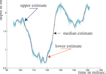
The first experiment is plotted in Figure 5, the second experiment is plotted in Figure 6. In all figures, the precise Butterworth filtered depth value is plotted in black and superimposed on the original signal (in cyan). The imprecise filtered value is plotted in red (lower value) and blue (upper value). When considering Figures 5 and 6, it can easily be seen that the precise filtered value belongs to the imprecise filtered value. The imprecise filtered value provided by the accounting-for-sampling approach is more specific than the possibilistic based approach. Moreover, when considering the possibilistic domination, the imprecision of the imprecise filtered value reflects the overall distance between the filtered signal and the original signal, providing a good measure of the
2 Sensor Technik Sirnach AG.
time in milisec.
depth in meter
.
Fig. 2. Raw depth signal.
time in milisec. ϕ
Fig. 3. Butterworth filter impulse response ϕ
noise level. Note that, with the Butterworth filter being a real-time filter (i.e. its impulse response is causal), the filtered signal is slightly delayed compared to the original signal. The same applies for the imprecise filtered signal.
5.2 Experimentation on derivating a signal
Signal derivation has been a great topic of interest in the image processing community since it is very useful for performing edge detection and image seg-mentation. Derivation consists generally of convolving a signal with a discrete
time in milisec. ϕ+
ϕ−
Fig. 4. Decomposition into two positive impulse responses ϕ+ and ϕ−
time in milisec. depth in meter . upper estimate lower estimate median estimate
Fig. 5. Depth signal filtered by the precise Butterworth filter (black) and the impre-cise possibility-based Butterworth filter (blue-upper, red-lower) superimposed with the original signal (cyan).
kernel obtained by sampling the derivative of an interpolative continuous ker-nel. In the image community, the Canny-Deriche filter is said to be optimal for edge detection since it respects Canny’s detection criteria. The Canny-Deriche derivative filter ϕ is given by: ϕi = −(1−β)
2
β iβ
|i|,where β ∈ [0, 1] is a parameter
that defines the filter bandwidth. The shape of the filter is depicted in Figure 7 for β ≃ 0, 4. This kernel can be considered as bounded by assuming that ϕi = 0 if |ϕi| ≤ ǫ, where ǫ represents the precision of the computer.
time in milisec. depth in meter . upper estimate lower estimate median estimate
Fig. 6. Depth signal filtered by the precise Butterworth filter (black) and the imprecise accounting-for-sampling capacity based Butterworth filter (blue-upper, red-lower) superimposed with the original signal (cyan).
time
magnitude of Deriche filter
anticausal part of the Deriche filter causal part of the Deriche filter time (a) (b)
Fig. 7. (a). Deriche and (b). Deiche canonical decomposition
a Canny Deriche filter and its imprecise version. This experiment aims at highlighting the usefulness of the dual Minkowsky difference in such a setting. Since most kernels used for derivation are positive and symmetric, the deriva-tion kernel is composed of two identical symmetric funcderiva-tions. The Canny-Deriche filter acts in the same way. Therefore, the canonical decomposition of the filter leads to ϕi = Aρi − Aρ−i, where ρ is a causal filter, i.e. such that
ρi = 0 if i < 0. Thus, let X = (Xn)n=1...N be the discrete signal to be filtered,
by: ˙
Xk= A(EPk+(X) − EPk−(X)), (6)
where P+
k (rsp. Pk− ) is the probability measure based on ρi (rsp. ρ−i ) at the
kth sample. E
Pk+(X) (rsp. EPk−(X)) can be seen as a right (rsp. left) mean value of signal X around the kth time sample. If these two mean values are
equal, then the derivative equals 0.
Now, let us consider two capacities v+ and v− and their respective cores.
The situation can arise that, for any P+ ∈ core(v+) and P− ∈ core(v−),
EP+
k (X) = EPk−(X) and therefore ˙Xk = 0 regardless of the considered prob-ability measure. However, there can be two probprob-ability measures P+, Q+
be-longing to core(v+), such that E
Pk+(X) 6= EQ +
k(X). Thus Ev+(X) = Ev−(X), but ˙Xk = A(Ev+(X) ⊖ Ev−(X)) 6= 0. When this situation occurs and if the capacity is chosen such that, usually Ev+(X) = Ev−(X) means that for any P+∈ core(v+) and P− ∈ core(v−), E
P+(X) = EP−(X), then the Minkowsky difference must be replaced by the dual Minkowsky difference in order to ob-tain a more specific (but also more risky) interval.
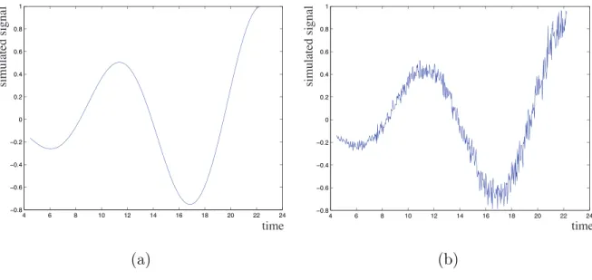
Let us consider the synthetic signal of the form x(t) = λtcos(wt) depicted in Figure 8.a and the same signal degraded by an additive gaussian noise whose standard deviation increases with time (i.e. the noise is not stationary), as depicted in Figure 8.b. time simulated signal time simulated signal (a) (b)
Fig. 8. Original signal without noise (a) and with noise (b).
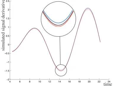
Since the signal is known, its derivative is also known, which enables us to illustrate the behavior of the derivation algorithm. Figures 9, 10, 11 and 12 present the derivative of both original (a) and noisy signals (b). In each figure, the real derivative is plotted in magenta, the precise estimated derivative is
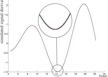
plotted in black while the imprecise derivative estimate is plotted in blue for upper and red for lower estimates. Figures 9 and 10 presents an imprecise estimate that uses the Minkowsky difference. Figures 11 and 12 present an imprecise estimate based on the dual Minkowski difference. In each Figure, we have expanded a specific detail of the signal (around time=14 ms.).
time
simulated signal derivative
Fig. 9. Derivative estimate of the original signal based on the Minkowsky difference.
time
simulated signal derivative
Fig. 10. Derivative estimate of the noisy signal based on the Minkowsky difference.
When comparing Figures 9 and 10 to Figures 11 and 12 it can easily be seen that the imprecise estimation of the derivative is always more precise when using the dual Minkowsky difference. This increased precision is an ad-vantage when the signal is not noisy, i.e. the only noise is due to sampling (Figures 8.a and 9): the dual Minkowsky difference based imprecise estimate, the precise estimate and the real derivative are almost identical. However, when the signal is noisy, the fact that the two intervals Ev+(X) and Ev−(X) are equal cannot be considered as a signature that, for any P+ ∈ core(v+)
time
simulated signal derivative
Fig. 11. Derivative estimate of the original signal based on the dual Minkowsky difference.
time
simulated signal derivative
Fig. 12. Derivative estimate of the noisy signal based on the dual Minkowsky dif-ference.
and P− ∈ core(v−), E
Pk+(X) = EPk−(X). Therefore, the imprecise estimate based on the dual Minkowsky difference can be seen as a too risky interval valued estimate since it does not always include the real derivative or the pre-cise estimated derivative (Figure 12). On contrary, when the filter is properly designed, the Minkowsky difference approach always includes the real signal (Figure 8.b). Moreover, the precise expected value is always included in the imprecise expected value due to Property 10.
6 Concluding remarks
In this paper, we have proposed a new interpretation and a new way of com-puting the imprecision associated with an observed value. According to this interpretation, the imprecision of an observation can be due to the observation process but also to poor knowledge on the proper post-processing to be used to filter the raw measured signal.
The conventional approach for signal filtering requires perfect knowledge of the proper function for modeling the impulse response of the filter to be used. However, such precise knowledge is usually difficult to justify, since it usually requires a lot of expert prior assumptions (shape of the function, identifica-tion criterion, data used in the identificaidentifica-tion process, etc.). In this article, we propose to extend this conventional approach by designing filtering tools that are able to account for imprecise knowledge of the impulse response of the filter. Our new filtering tool is based on replacing a single precise impulse response by a set of impulse responses that is consistent with the user’s expert knowledge. Our approach is based on considering the usual linear filtering as a linear combination of two expectation operations and extending these ex-pectation operations to concave capacities. We have proposed straightforward methods to enable a user to design capacities that are likely to represent the convex hull of all the saught-after impulse reponses. Several properties of this approach have been proved that show its consistency with the conventional approach. Particularly, when considering the Minkowski sum-based extension, the imprecise output of our filter contains all outputs of the filters whose im-pulse response belongs to the considered convex hull. However, as mentionned in the article, this output can be too imprecise, i.e. it contains output signals that are not outputs of the set of filters envisaged by the user. Thus, we also considered another approach based on the dual Minkowski sum. However, this approach can lead to a too specific filtered output. In fact, the filter output can be guaranteed to be the most specific interval-valued output only when all the considered impulse responses are either positive or negative. Future work should be focused on finding a way to design a method that can ensure this property for sets of impulse reponses that are both negative and positive (which is the most general case). Note that our actual approach only considers a precise signal input. It would be useful to consider extending our work to an imprecise signal input, whose imprecision comes from a previous imprecise filtering or is due to pre-calibration of the expected signal error.
7 Acknowledgement
The authors are indebted to Olivier Parodi for the pressure data used in this article.
References
[1] C. Baudrit and D. Dubois. Practical representations on incomplete probabilistic knowledge. Computational Statistics and Data Analysis, 51(1):86–108, 2006. [2] L. Campos, J. Huerte, and S. Moral. Probabilities intervals: a tool of uncertainty
reasoning. International Journal of Uncertainty, Fuzzyness and
Knowledge-Based Systems, 2:167–196, 1994.
[3] E. Jack Chen and W. David Kelton. Quantile and tolerance-interval estimation in simulation. European Journal of Operational Research, 127(2):520–540, January 2006.
[4] G. Chen, J. Wang, and L. Shieh. Interval kalman filtering. IEEE Transactions
on Aerospace and Electronic Systems, 33(1):250–259, 1997.
[5] D. Denneberg. Non-Additive Measure and Integral. Kluwer Academic Publishers, 1994.
[6] D. Dubois. Possibility theory and statistical reasoning. Computational Statistics
and Data Analysis, 51(1):47–69, 2006.
[7] M. Grabisch and Ch. Labreuche. The symmetric and asymmetric choquet integrals on finite spaces for decision making. Statistical Papers, 43:37–52, 2002. [8] M. Hadj-Sadok and J. Gouz´e. Estimation of uncertain models of activated sludge processes with interval observers. Journal of Process Control, 11(3):299– 310, 2001.
[9] J. Hall and J. Lawry. Generation, combination and extension of random set approximations to coherent lower and upper probabilities. Reliability Engeneering and System Safety, 85(1-3):89–101, 2004.
[10] Masuo Hukuhara. Int´egration des applications mesurables dont la valeur est un compact convexe. In Funkcialaj Ekvacioj, volume 10, pages 205–223, 1967. [11] L. Jaulin, M. Kieffer, O. Didrit, and E. Walter. Applied Interval Analysis with
Exemples in Parameter ans State Estimation, Robust Control and Robotics. Springer, 2001.
[12] Luc Jaulin and Eric Walter. Set inversion via interval analysis for nonlinear bounded-error estimation. Automatica, 29(4):1053–1064, 1993.
[13] V. Kreinovich and S. Ferson. A new cauchy-based black box technique for uncertainty in risk analysis. Reliability Engeneering and System Safety, 85(1-3):267–279, 2004.
[14] V. Kreinovich and S. Ferson. Comuting best-possible bounds for the distribution of a sum of several variables is np-hard. International Journal of Approximate
reasoning, 41(3):331–342, 2006.
[15] Vladik Kreinovich, Luc Longpr´e, Scott A. Starks, Gang Xiang, Jan Beck, Raj Kandathi, Asis Nayak, Scott Ferson, and Janos Hajagos. Interval versions of statistical techniques with applications to environmental analysis, bioinformatics, and privacy in statistical databases. J. Comput. Appl. Math., 199(2):418–423, 2007.
[16] K. Loquin and O. Strauss. On the granularity of summative kernels. Fuzzy Sets
and Systems, 159(15):1952–1972, 2008.
[17] J. Nankervis. Computational algorithms for double bootstrap confidence intervals. Computational Statistics and Data Analysis, 49(2):461–475, 2005. [18] P.Walley. Statistical reasoning with imprecise probabilities. Chapman and Hall,
New-York, 1991.
[19] J. Serra. Image analysis and mathematical morphology. London, 1982.
[20] J.M. Spiewak, B. Jouvencel, and P. Fraisse. A new design of auv for shallow water applications:h160. In International Offshore and Polar Engineering, 2006. [21] M. Unser, A. Aldroubi, and M. Eden. B-spline signal processing: Part i-theory.
IEEE Transactions on Signal Processing, 41:821–833, 1993.
[22] H. Vald`es-Gonzalez, J-M Flaus, and G. Acuna. Moving horizon state estimation with global convergence using inteval tecniques: application to biotechnological processes. Journal of Process Control, 13(4):325–336, 2003.
[23] R. Yager and V. Kreinovich. Decision making under interval probabilities.
International Journal of Approximate Reasoning, 22:195–215, 1999.
[24] Y. Zhu and B. Li. Optimal interval estimation fusion based on sensor interval estimates with confidence degrees. Automatica, 42:101–108, 2006.